Low and high frequency intracranial neural signals match in the human associative cortex
- Université de Lorraine, CNRS, CRAN, France
- Psychological Sciences Research Institute (IPSY), Université Catholique de Louvain (UCLouvain), Belgium
- Université de Lorraine, CHRU-Nancy, Service de Neurologie, France
- Université de Lorraine, CHRU-Nancy, Service de Neurochirurgie, France
Figures
Figure 1
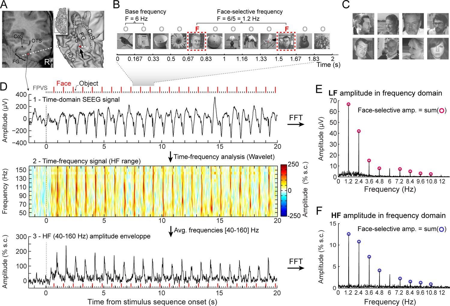
Recording and quantifying SEEG low frequency (LF) and high frequency (HF) face-selective signals in the VOTC.
(A) Left: Coronal slice of an example depth (SEEG) electrode implanted in the right VOTC of an individual participant. Right: the same SEEG electrode array is shown on the reconstructed white matter surface of the participant (ventral view of the right hemisphere). Intracerebral electrode arrays consist of 5–15 contiguous recording contacts (small white rectangles in the coronal slice, white circles on the 3D surface) spread along the electrode length. Electrodes penetrate both gyral and sulcal cortical tissues. Here the electrode extends from the fusiform gyrus to the middle temporal gyrus. The recording contact located at the junction between the lateral fusiform gyrus and occipito-temporal sulcus and where the signal shown in panels D-F is measured is highlighted in red (left: red rectangles surrounded by a circle; right: red circles, see the black arrow). Acronyms: CoS: Collateral sulcus; OTS: Occipito-temporal sulcus; FG: Fusiform gyrus; IOG: Inferior occipital gyrus. (B) The fast periodic visual stimulation (FPVS) (or frequency-tagging) paradigm to quantify face-selective neural activity (originally from Rossion et al., 2015; see e.g., Jacques et al., 2016a; Rossion et al., 2018): natural images of nonface objects are presented by sinusoidal contrast modulation at a rate of six stimuli per second (6 Hz) with highly variable face images presented every five stimuli. Common neural activity to faces and nonface objects is expressed at 6 Hz and harmonics in the iEEG signals, while selective (i.e., differential) activity elicited reliably by face stimuli appears at the frequency of 6/5=1.2 Hz. Each stimulation sequence lasts for 70s (2 s showed here). (C) Representative examples of natural face images used in the study (actual images not shown for copyright reasons). (D) Top: example raw intracranial EEG time-domain signal measured at the recording contact shown in panel A. The signal is shown from –1.5 to 20 s relative to the onset of a stimulation sequence. The time-series displayed is an average of 2 sequences. Above the time-series, red vertical ticks indicate the appearance of face image in the sequence every 0.835 s (i.e. every 5 image at 6 Hz) and small black vertical ticks indicate the appearance of non-face objects every 0.167 s. Example images shown in each sequence are shown in panel B. Middle: a time-frequency representation of the SEEG data in the HF range (40–160 Hz) is obtained with a wavelet transform. The plot shows the percent signal change at each frequency relative to a pre-stimulus baseline period (–1.6s to –0.3s). This highlights distinct periodic burst of HF activity occurring at the frequency of face stimulation (i.e. 1.2 Hz) after the start of the stimulation sequence. Bottom: The modulation of HF amplitude over time (i.e. HF amplitude envelope) is obtained by averaging time-frequency signals across the 40–160 Hz frequency range. Red vertical ticks indicate the appearance of face images in the sequence. (E) LF face-selective amplitude is quantified by transforming the time-domain iEEG signal to the frequency domain (Fast Fourier Transform, FFT) and summing amplitudes of the signal at 12 harmonics of the frequency of face stimulation (1.2, 2.4, 3.6, 4.8, … Hz, excluding harmonics of the 6 Hz base stimulation rate). (F) HF face-selective amplitude is quantified in the same manner as for LF (panel E) with FFT applied to the HF amplitude envelope.
Figure 2 with 3 supplements
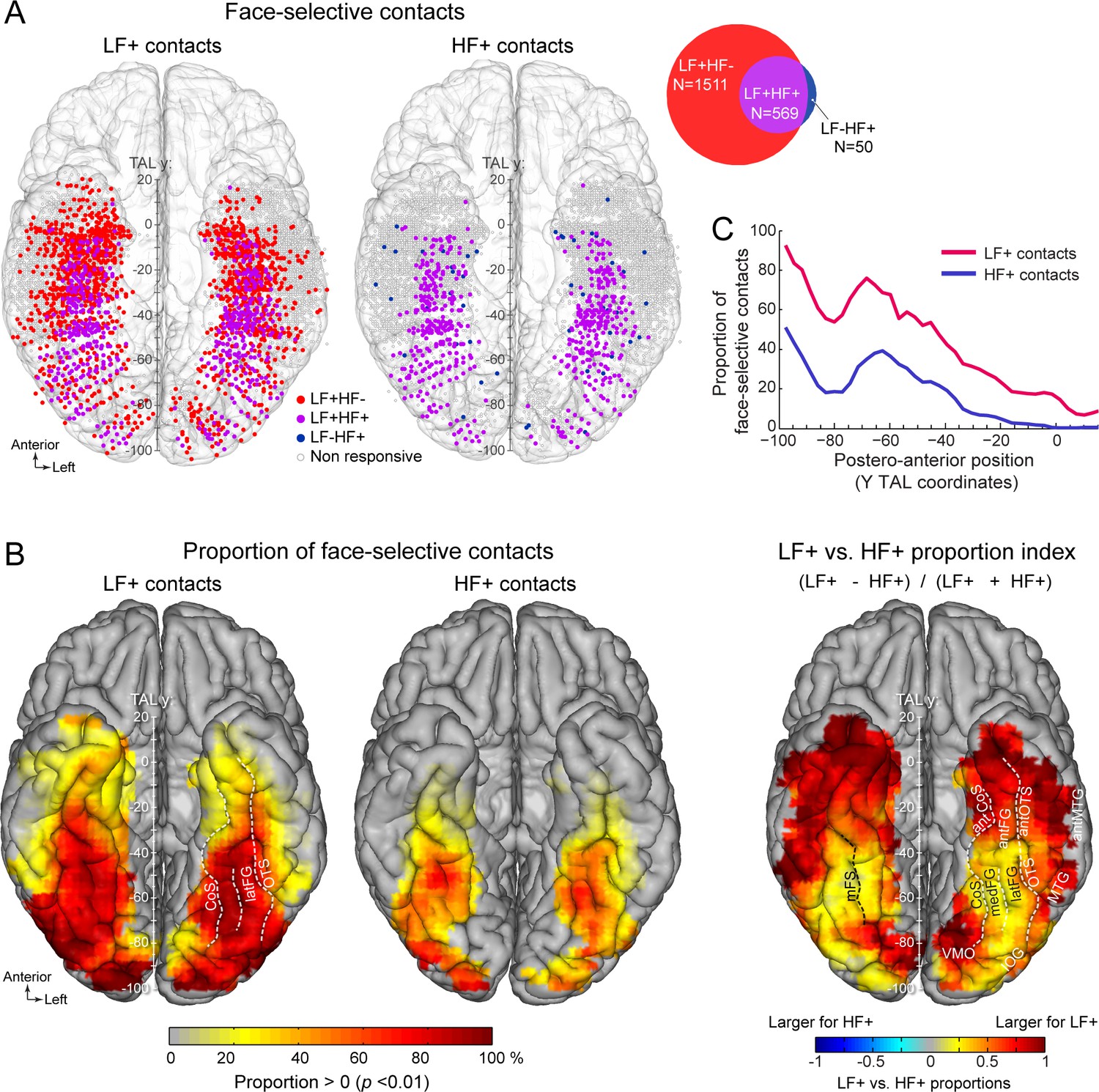
Spatial distribution and proportion of LF and HF face-selective SEEG activity over VOTC.
(A) Map of all VOTC recording contacts across the 121 individual brains displayed in the Talairach space using a transparent reconstructed cortical surface of the Colin27 brain (ventral view). Each circle represents a single recording contact. Each color-filled circle corresponds to a face-selective contact colored as a function of whether LF and/or HF activity is significant (z-score >3.1, p<00.1) at the contact (for contact count see Venn diagram inset on the right). White-filled circles correspond to contacts on which no significant face-selective activity was recorded. For visualization purposes, individual contacts are displayed larger than their actual size (2 mm in length). Values along the y-axis of the Talairach coordinate system (antero-posterior) are shown near the interhemispheric fissure. (B) VOTC maps of the local proportion of contacts showing significant face-selective activity in LF irrespective of HF (LF+, left) and HF irrespective of LF (HF+, middle) relative to the number of recorded contacts, as well as the comparison between the local proportions of LF+ and HF+ contacts across VOTC (right). Proportions are computed using recording contacts contained in 12x12 mm (for x and y Talairach dimensions) voxels. For left and middle maps, only local proportions significantly above zero (p<0.01, percentile bootstrap) are displayed. The map on the right shows an index comparing LF+ to HF+ local proportions computed as the ratio of the proportions of LF+ minus HF+ over the sum of these proportions. Positive values indicate larger proportion of LF+ contacts. (C) Proportion of face-selective LF+ and HF+ contacts as a function of the position along the y Talairach axis (postero-anterior) computed by collapsing contacts over both hemispheres. See also Figure 2—figure supplement 1, Figure 2—figure supplement 2, .
Figure 2—figure supplement 1

Number and proportion of significant face-selective contacts by anatomical region.
(A) The number of face-selective contacts is show for each contact type (i.e. determined by whether or not LF or HF signal is significant in each contact), in each anatomical region (region defined in each individual participant) and hemisphere. (B) Proportion of each contact type computed for each region and hemisphere.
Figure 2—figure supplement 2
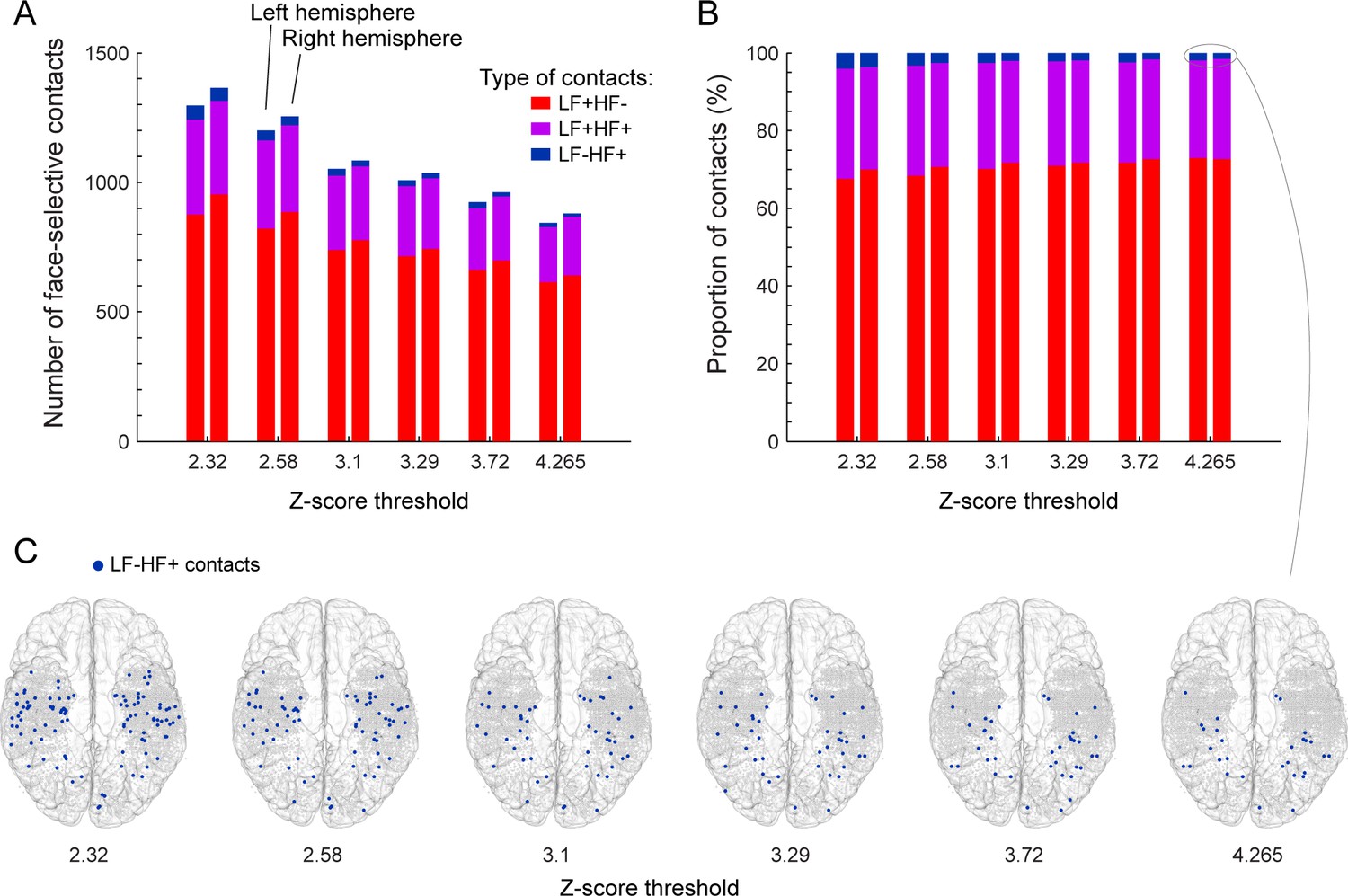
Number and proportion of significant face-selective contacts as a function of statistical threshold.
(A) Number of each type of contacts as a function of the z-score threshold used to detect a significant face-selective response. (B) Proportion of each type of contact as a function of z-score threshold. C. VOTC maps showing the location of LF-HF+ contacts (i.e. contact with significant face-selective responses in HF only) as a function z-score threshold.
Figure 2—figure supplement 3

Labeling face-selective contacts in the individual brain anatomy.
(A). Anatomical regions were defined in each individual hemisphere according to major anatomical landmarks. The ventral temporal sulci (COS, OTS, and midfusiform sulcus, i.e., MFS) serve as medial/lateral borders of regions, whereas three coronal reference planes containing anatomical landmarks (posterior tip of the hippocampus, that isi.e., HIP, anterior tip of the parieto-occipital sulcus, i.e., POS, limen insulae) serve as an anterior/posterior boundary for each region. We considered contacts in the ATL if they were located anteriorly to the posterior tip of the hippocamps and posteriorly to the limen insulae. The schematic locations of these anatomical structures are shown on a reconstructed cortical surface of the Colin27 brain. Acronyms: TP: temporal pole; ATL: anterior temporal lobe; PTL: posterior temporal lobe; OCC: occipital lobe; PHG: parahippocampal gyrus; CoS: collateral sulcus; FG: fusiform gyrus; ITG: inferior temporal gyrus; MTG: middle temporal gyrus; OTS: occipito-temporal sulcus; CS: calcarine sulcus; IOG: inferior occipital gyrus; LG: lingual gyrus; ant: anterior; lat: lateral; med: medial. (B) Map of all face-selective recording contacts pooled across LF+ and HF+ signals and displayed in the Talairach space. Each circle represents a single face-selective contact color-coded according to its anatomical location in the original individual anatomy (see legend on the right).
Figure 3
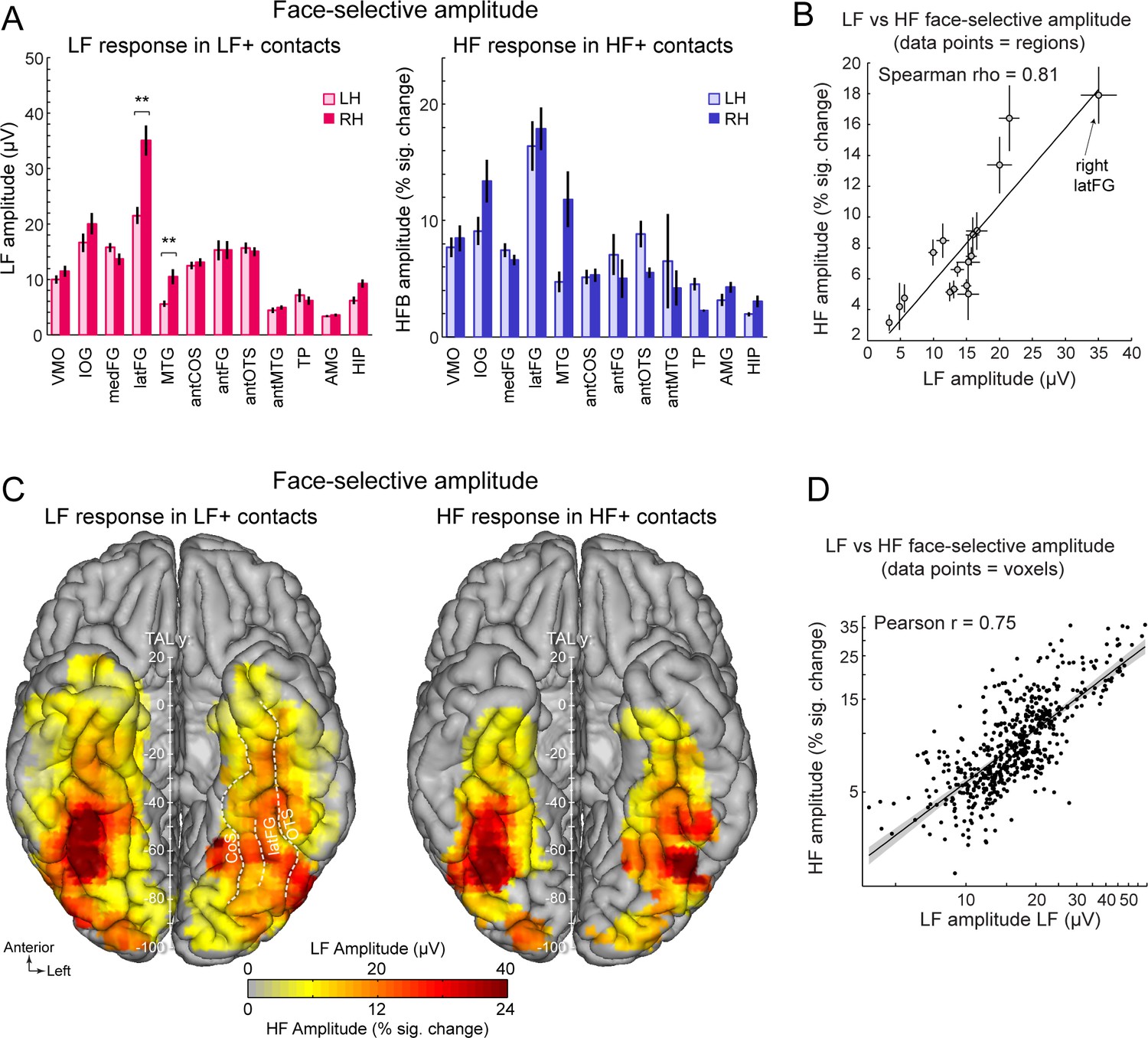
Face-selective LF and HF amplitude quantification.
(A) LF face-selective amplitudes in LF+ contacts (left) and HF amplitude in HF+ contacts shown for each anatomical region (i.e., as defined in the individual native anatomy) and separately for the left and right hemispheres (LH and RH, respectively). Amplitudes are quantified as the mean of the amplitudes across recording contacts within a given anatomical region. Error bars are standard error of the mean across contacts (see Table 1 for sample size in each region). (B) Scatter plot revealing the similarity in the patterns of face-selective LF and HF amplitudes measured in each anatomical region. The amplitude values are the same as in panel A, excluding HIP and TP for which there were too few HF+ contacts. (C) Maps showing smoothed LF face-selective amplitude over LF+ contacts (left) and HF amplitude over HF+ contacts (right) displayed over the VOTC cortical surface. Amplitudes are averaged over contacts in 12x12 mm voxels. Only voxels with a proportion of face-selective contact significantly above zero (p<0.01, percentile bootstrap) are displayed. (D) Linear relationship between LF and HF amplitude maps shown in panel C. Each data point shows the face-selective amplitude in LF and HF in a 12x12 mm voxels in Talairach space. Amplitudes were normalized using log transformation prior to computing the Pearson correlation. Only voxels overlapping across the two maps are used to estimate the Pearson correlation. The shaded area shows the 95% confidence interval of the linear regression line computed by resampling data points with replacement 1000 times.
Figure 4 with 3 supplements
Manipulating statistical threshold for LF+ and HF+ contacts.
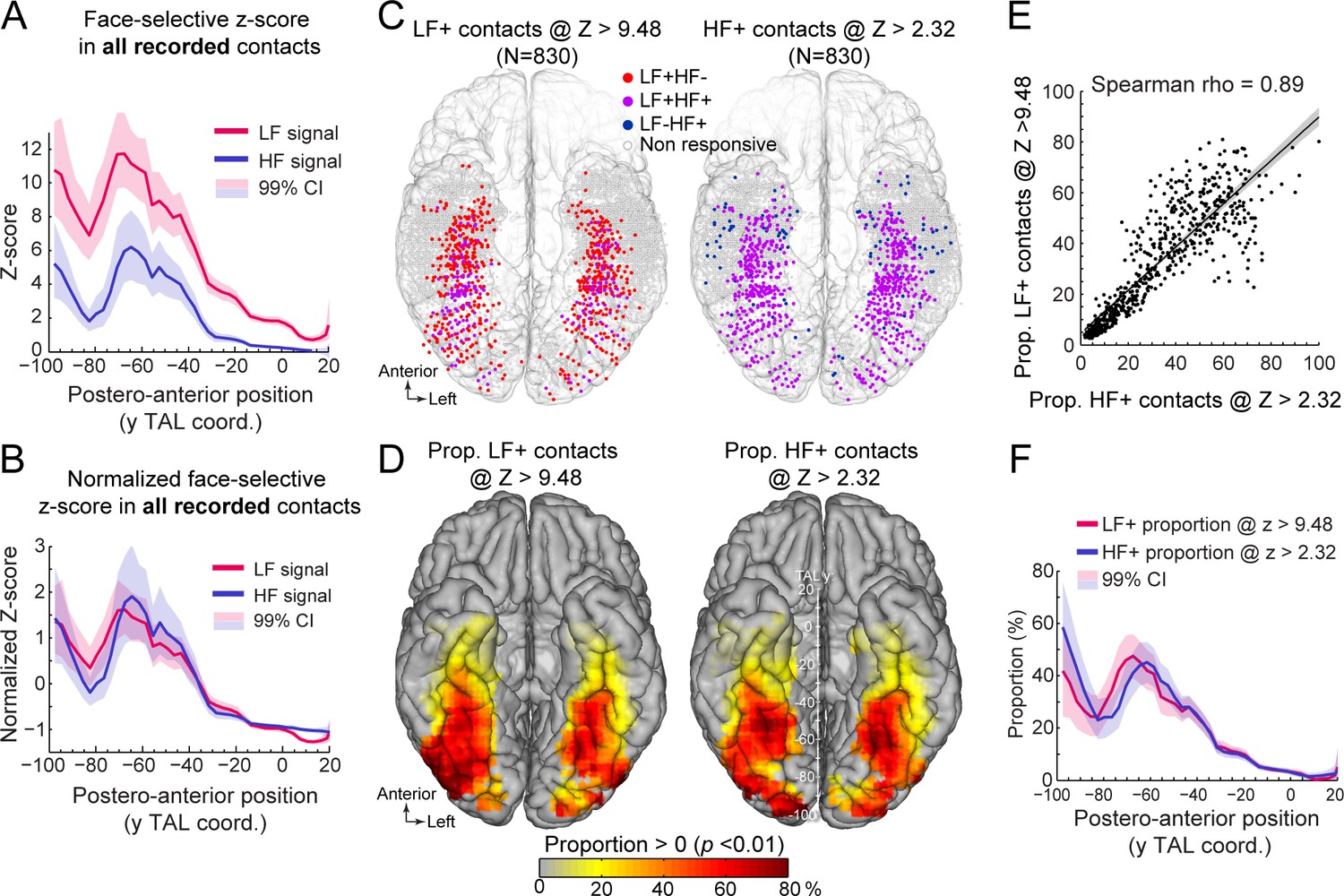
(A) Postero-anterior Z-score profiles for LF and HF signals. Z-scores for the face-selective activity measured over all recorded VOTC contacts (i.e. N=7374 contacts) are displayed as a function of the position along the y Talairach axis (postero-anterior; computed by taking the mean Z-score over contacts collapsed across both hemispheres). (B) Postero-anterior Z-score profiles (same as in panel A) normalized independently for LF and HF (subtracting the mean and dividing by the standard deviation across postero-anterior positions) to highlight their similarity. (C) Spatial distribution of LF+ (left) and HF+ (right) contacts across VOTC after varying the Z-score statistical thresholds (Z>9.48 for LF+ and Z>2.32 for HF+) to equalize the number of recording contacts exhibiting a significant response (i.e. N=830). Color-filled vs. white-filled circle are contacts with vs. without significant face-selective activity at the target Z-score threshold. (D) VOTC maps of the local proportion of LF+ (left) and HF+ (right) face-selective contacts detected at two different Z-score thresholds to equalize the number of significant contacts (see panel C). Only local proportions significantly above zero (p<0.01) are displayed. (E) Scatter plot displaying the strong similarity between LF+ and HF+ proportion maps shown in panel D. Each data point is the proportion of LF +vs HF+ contacts (i.e., detected using two different Z-score threshold) in a 12x12 mm voxels in Talairach space. Only voxels overlapping across the two maps are used to estimate the correlation. The shaded area shows the 95% confidence interval around the linear regression line (computed by resampling data points with replacement 1000 times). (F) Postero-anterior profile of LF+ and HF+ proportions with two different Z-score thresholds (see panels C, D). See also Figure 4—figure supplement 1, Figure 4—figure supplement 2.
Figure 4—figure supplement 1
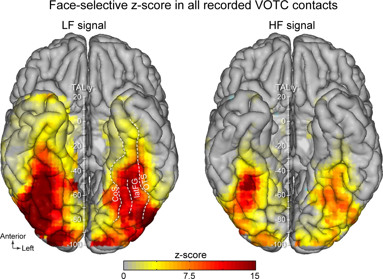
VOTC maps of face-selective z-scores on all recorded contacts.
VOTC maps displaying the local mean face-selective z-score computed over ALL recorded contacts (i.e. whether or not contacts are face-selective) within 12x12 mm voxels for LF signal (left) and HF signal (right). The mean face-selective z-score is generally higher for LF signal. For both LF and HF signals, the z-score is lowest in the anterior part of the temporal lobe.
Figure 4—figure supplement 2
Manipulating statistical threshold to equate number of LF+ and HF+ contacts (using alternative z-score thresholds compared to Figure 5).
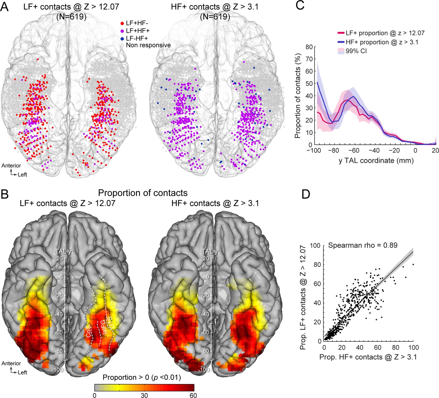
(A) Spatial distribution of LF+ (left) and HF+ (right) contacts across VOTC after manipulating the z-score statistical thresholds (Z>12.07 for LF+ and Z>3.1 for HF+) to equalize the number of recording contacts exhibiting a significant response (i.e. N=619). Color-filled vs. white-filled circle are contacts with vs. without significant face-selective response at the target z-score threshold. (B) VOTC maps of the local proportion of LF+ (left) and HF+ (right) face-selective contacts detected at two different z-score thresholds to equalize the number of significant contacts (see panel A). Only local proportions significantly above zero (p<0.01) are displayed. (C) Postero-anterior profile of LF+ and HF+ proportions when using two different z-score thresholds (see panels A, B). (D) Linear relationship between LF+ and HF+ proportion maps shown in panel B. Each data point is the proportion of LF +vs HF+ contacts (i.e. detected using two different z-score threshold) in a 12x12 mm voxels in Talairach space. Only voxels overlapping across the two maps are used to estimate the Pearson correlation. Shaded area show the 95% confidence interval of the linear regression line computed by resampling data points with replacement 1000 times.
Figure 4—figure supplement 3
Exploring the role of signal and noise in variations of Z-score across signals and VOTC regions.
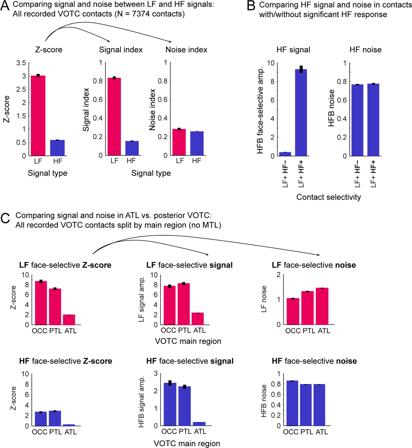
To understand the origin of the difference in signal-to-noise ratio (computed as a z-score in the current study) between LF and HF electrophysiological signals, we decomposed the z-score into its ‘signal’ and ‘noise’ constituents. (A) We addressed the lower z-score for HF compared to LF (left plot) by computing face-selective signal and noise collected over all recorded VOTC contacts (N=7374,, excluding contacts in the white matter). We used all recorded contacts to avoid any potential bias resulting from the use of only contacts with a significant response (i.e. having z-score >3.1). To directly compare signal and noise across signals we computed a ‘signal index’ (middle plot) and a ‘noise index’ (right plot) for each recording contact that accounts for the 1/f relationship between EEG amplitude and frequency and differences in the unit used for LF and HF (µV vs. percent signal change). Specifically, the signal and noise indices were computed as follows: (1) fft spectrum was segmented in 4 segments of 51 bins centered around the first 4 harmonics of the face-selective frequency (1.2–4.8 Hz, similarly as for the computation of the z-score); (2) we summed the 4 segments; (3) based on the summed segments we compute (a) the ‘raw face-selective amplitude’ as the amplitude at the face-frequency (i.e. at the center of the summed segment), (b) the ‘amplitude of the baseline’ as the mean amplitudes in the 48 bins surrounding the face-frequency bin (i.e. excluding the 2 bins immediately adjacent to the face frequency bin), (c) ‘the baseline-subtracted amplitude’ as the difference between the raw face-selective amplitude and the amplitude of the baseline, (d) ‘the standard deviation of the noise’ as the standard deviation of the amplitude in the 48 bins surrounding the face frequency; (4) from these values we compute the signal index as the baseline-subtracted amplitude divided by the amplitude of the baseline, and the noise index as the standard deviation of the noise divided by the amplitude of the baseline. This revealed that the face-selective signal amplitude was on average almost 5 times larger for LF compared to HF (middle plot: mean +/- std: 0.83+/-1.34 for LF vs. 0.15+/-0.45 for HF) while the noise was much more similar across the two types of signals (right plot: 0.28+/-0.03 for LF vs. 0.26+/-0.03 for HF). This indicates that the lower z-score for HF compared to LF is driven by a smaller face-selective signal, and not by a higher noise for HF. (B) Similarly, we also compare the face-selective HF signal amplitude (i.e. HF baseline-subtracted amplitude as described for panel A) and HF noise (i.e. HF standard deviation of the noise as described for panel A) across LF+ contacts with or without significant HF face-selective response. These contacts differ in terms signal amplitude (0.40+/-0.87 for LF+ HF vs. 9.32+/-9.13 for LF+ HF) rather than in terms of noise (0.77+/-0.28 for LF+ HF vs. 0.77+/-0.22 for LF+ HF-). (C) To investigate the overall lower z-score in the ATL compared to more posterior VOTC region (left plot, top row: LF signal; bottom row: HF signal), we computed LF and HF signal (i.e. baseline-subtracted amplitude as described for panel A) and noise (i.e. standard deviation of the noise as described for panel A) in 3 main regions of the VOTC (OCC, PTL, ATL), again using all recorded VOTC contacts (excluding contacts in the MTL). This revealed that the mean face-selective signal amplitude within the ATL was 72% (LF) and 92% (HF) smaller than in the PTL (middle plot). In contrast, the noise in the ATL was only 10% larger (LF) or of equal magnitude (HF) than in the PTL (right plot). This indicates that the lower z-scores in ATL are mostly driven by a smaller face-selective signal amplitude in this region compared to the posterior VOTC.
Figure 5 with 5 supplements
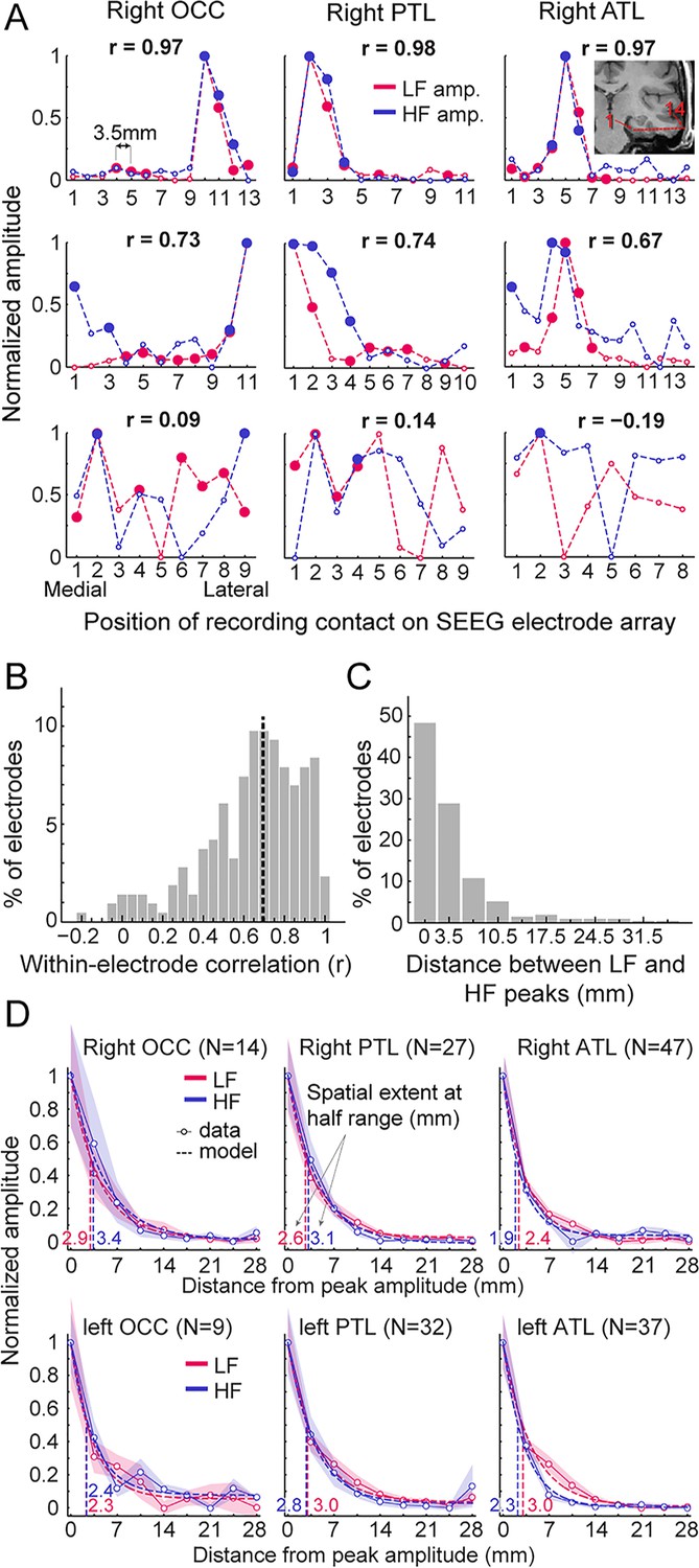
Local spatial extent of LF and HF signals.
(A) Face-selective LF and HF amplitude (normalized between 0 and 1 for display) measured at each contact along a few examples of whole SEEG electrode arrays in the three main right hemisphere VOTC regions (columns). The schematic anatomical trajectory of an ATL electrode is depicted in the inset in the upper right plot. Each plot displays LF and HF signals over the same electrode. Filled circles indicate contacts with significant face-selective activity (Z>3.1). Only electrodes containing at least one LF+HF+ contact are included. Plots are vertically ordered by similarity between LF and HF amplitude profiles along the SEEG electrode (quantified using Pearson’s correlation): from electrodes with the highest coefficient (top row, see Pearson’s r coefficient at the top of each plot), to median (middle row) and worst correlations (bottom row). (B) Histogram of Pearson correlations computed between LF and HF amplitudes within each SEEG electrode (N=215 electrodes, see example correlations in panel A). Median correlation is represented by the vertical dashed line. (C) Histogram of the distance between LF and HF peak amplitude in any given electrode array. For 48% of all electrodes, the peak amplitude for LF and HF occurred on the same contact (e.g. top row of panel A) and for 29% LF and HF peak amplitudes occur at directly adjacent contacts (e.g. middle row, right column in panel A). (D) Local spatial extent of face-selective LF and HF signals in each main VOTC region. Each plot displays the mean variation of face-selective LF and HF amplitude as a function of the distance (mm) from the peak amplitude (located at 0 mm). Only electrodes where LF and HF peak amplitude were at most 3.5 mm from each other were used (see electrode count for each region in parenthesis). Mean amplitudes have been normalized between 0 and 1 for display only; all analyses being performed on non-normalized data. The spatial extent was estimated for each signal and main region by fitting an exponential decay function (dashed lines) to the mean amplitude profile (thin lines) and finding the distance at which the function reach half of its amplitude range. Resulting spatial extents are indicated on each plot and marked by vertical dashed lines. Shaded areas are the standard error of the mean across electrode arrays. See also Figure 5—figure supplement 1, Figure 5—figure supplement 2, Figure 5—figure supplement 3, Figure 5—figure supplement 4, Figure 5—figure supplement 5.
Figure 5—figure supplement 1

LF and HF amplitude along SEEG electrode arrays: right OCC and right PTL.
Face-selective LF and HF amplitude (normalized between 0 and 1 for display) measured at each face-selective contact along the whole SEEG electrode array. Electrodes are grouped by main VOTC regions and hemispheres. Each plot displays LF and HF signal over the same electrode. Only electrode containing at least one LF+HF+ contact are included. Plots are ordered by Pearson correlation between LF and HF amplitude along the SEEG electrode: from the electrode with the highest correlation (top left, see Pearson’s r coefficient at the top of each plot), to the worst correlation (bottom right). Filled circles indicate contacts with significant face-selective response (Z>3.1).
Figure 5—figure supplement 2
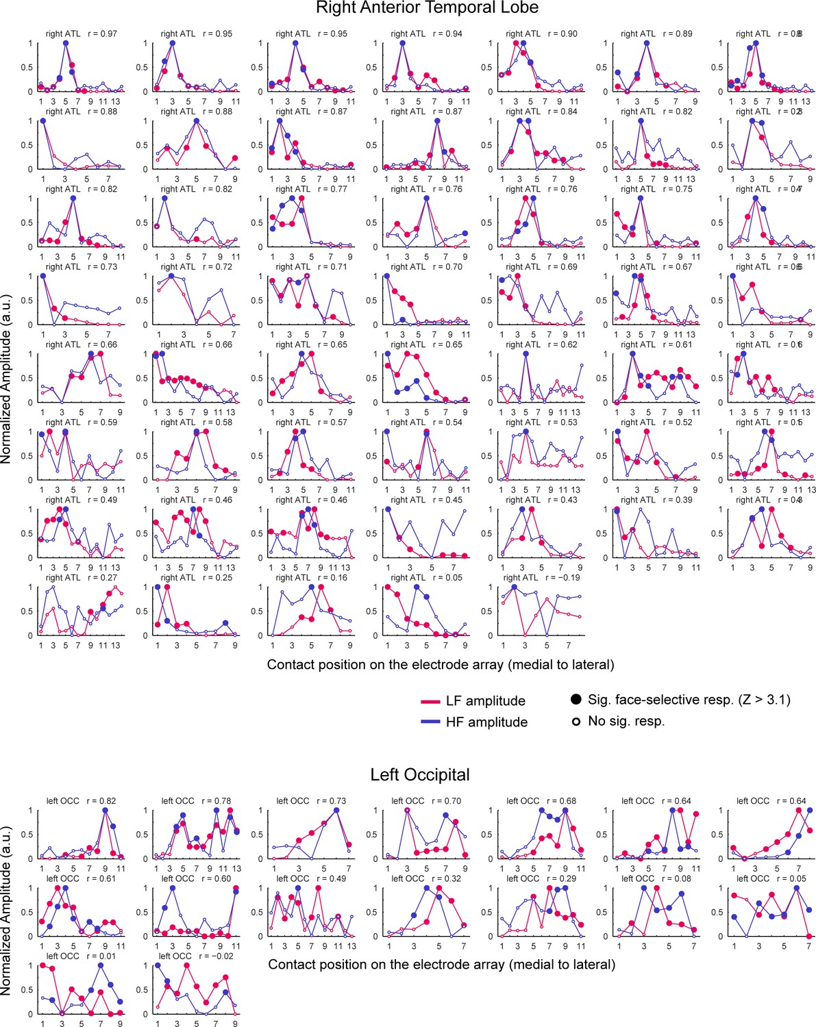
LF and HF amplitude along SEEG electrode arrays: right ATL and left OCC.
Figure 5—figure supplement 3
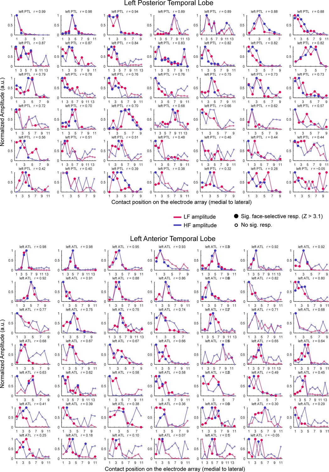
LF and HF amplitude along SEEG electrode arrays: left PTL and left ATL.
Figure 5—figure supplement 4
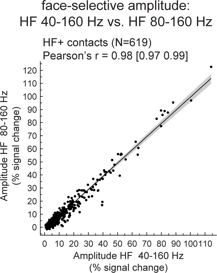
Scatter plot showing the linear relationship between HF face-selective amplitude measured in the 40–160 Hz frequency range and in the 80–160 Hz frequency range.
Data points are HF+ contacts selected based on the 40–160 Hz signal (N=619). Pearson’r and 99% confidence interval are indicated on top of the plot.
Figure 5—figure supplement 5
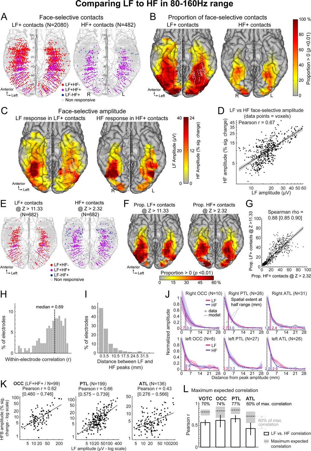
Comparing LF signal to HF signal measured over the 80–160 Hz range.
Significant contacts in the HF range were determined in the same manner as in the main analyses but using HF signal averaged over 80–160 Hz. This resulted in 482 HF+ contacts. The figure shows that measuring HF over 80–160 Hz frequency range results in extremely similar observations as when HF is measured over 40–160 Hz range. Most analyses have been replicated using 80–160 Hz frequency range. More details on methods and extended captions appear in the main manuscript. (A) Related to Figure 2. Spatial distribution of recording contacts (Talairach space over Colin27 brain) showing significant (z-score >3.1) face-selective activity in LF (left) and HF (80–160 Hz, right) (B) Related to Figure 2. VOTC maps of the local proportion of contacts showing significant face-selective activity in LF irrespective of HF (LF+, left) and HF irrespective of LF (HF+, middle) relative to the number of recorded contacts. Only local proportions significantly above zero (P<0.01) are displayed. (C) Related to Figure 3. Maps showing smoothed LF face-selective amplitude over LF+ contacts (left) and HF amplitude over HF+ contacts (right) displayed over the VOTC cortical surface. Amplitudes are averaged over contacts in 12x12 mm voxels. Only voxels with a proportion of face-selective contact significantly above zero (p<0.01, percentile bootstrap, Figure 3B) are displayed. (D) Related to Figure 3. Linear relationship between LF and HF amplitude maps shown in panel C. Each data point shows the face-selective amplitude in LF and HF in a 12x12 mm voxels in Talairach space. Amplitudes were normalized using log transformation prior to computing the Pearson correlation. (E) Related to Figure 4. Spatial distribution of LF+ (left) and HF+ (right) contacts across VOTC after manipulating the z-score statistical thresholds (Z>11.33 for LF+ and Z>2.32 for HF+) to equalize the number of recording contacts exhibiting a significant response (i.e. N=682). (F) Related to Figure 4. VOTC maps of the local proportion of LF+ (left) and HF+ (right) face-selective contacts detected at two different Z-score thresholds to equalize the number of significant contacts (see panel E). Only local proportions significantly above zero (p<0.01) are displayed. (G) Scatter plot displaying the linear relationship between LF+ and HF+ proportion maps shown in panel F. Each data point is the proportion of LF +vs HF+ contacts (i.e. detected using two different Z-score threshold) in a 12x12 mm voxels in Talairach space. Only voxels overlapping across the two maps are used to estimate the correlation. (H) Histogram of Pearson correlations computed between LF and HF amplitudes within each SEEG electrode (N=168 electrodes). Median correlation is represented by the vertical dashed line. (I) Histogram of the distance between LF and HF peak amplitude in any given electrode array. For 49% of all electrodes, the peak amplitude for LF and HF occurred on the same contact and for 27% LF and HF peak amplitudes occur at directly adjacent contacts. (J) Local spatial extent of face-selective LF and HF signals in each main VOTC region. Each plot displays the mean variation of face-selective LF and HF amplitude as a function of the distance (mm) from the peak amplitude (located at 0 mm). The spatial extent was estimated for each signal and main region by fitting an exponential decay function (thin lines) to the mean amplitude profile (dashed lines) and finding the distance at which the function reach half of its amplitude range. There was no significant difference between LF and HF in any region, except in the left ATL (p<0.01, two-tailed permutation test, fdr-corrected). (K) Scatter plot showing the linear relationship between log-transformed LF and HF face-selective amplitude split by main anatomical region, using LF+ HF+ recording contacts as data points. (L) Pearson correlation coefficients (white bars) are compared to estimations of the maximum correlation that could is expected given the presence of noise in the data (dotted horizontal lines). Error bars and shaded area around the maximum expected correlation (MEC) are 99% confidence intervals. On top of each bar, the ratio of actual correlation to the MEC indicates the percentage of the maximum correlation obtained in each region.
Figure 6
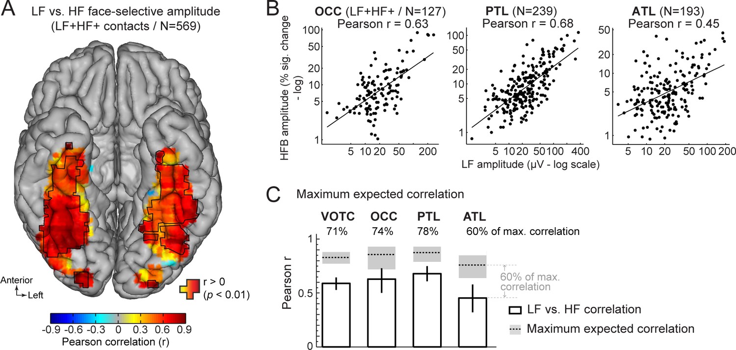
Functional relationship between LF and HF face-selective responses.
(A) VOTC map of Pearson correlations computed between LF and HF face-selective amplitude (log-transformed) measured in LF+HF+ recording contacts. Correlations were computed using contacts located in 15x15 mm voxels. Only voxels containing at least 9 recording contacts are displayed. Significant correlations (p<0.01) are outlined by black contours. (B) Scatter plot showing the linear relationship between log-transformed LF and HF face-selective amplitude split by main anatomical region, using LF+HF+ recording contacts as data points. (C) Pearson correlation coefficients (white bars) are compared to estimations of the maximum correlation that is expected given the presence of noise in the data (dotted horizontal lines). Error bars and shaded area around the maximum expected correlation (MEC) are 99% confidence intervals. On top of each bar, the ratio of actual correlation to the MEC indicates the percentage of the maximum possible correlation obtained in each region.
Figure 7
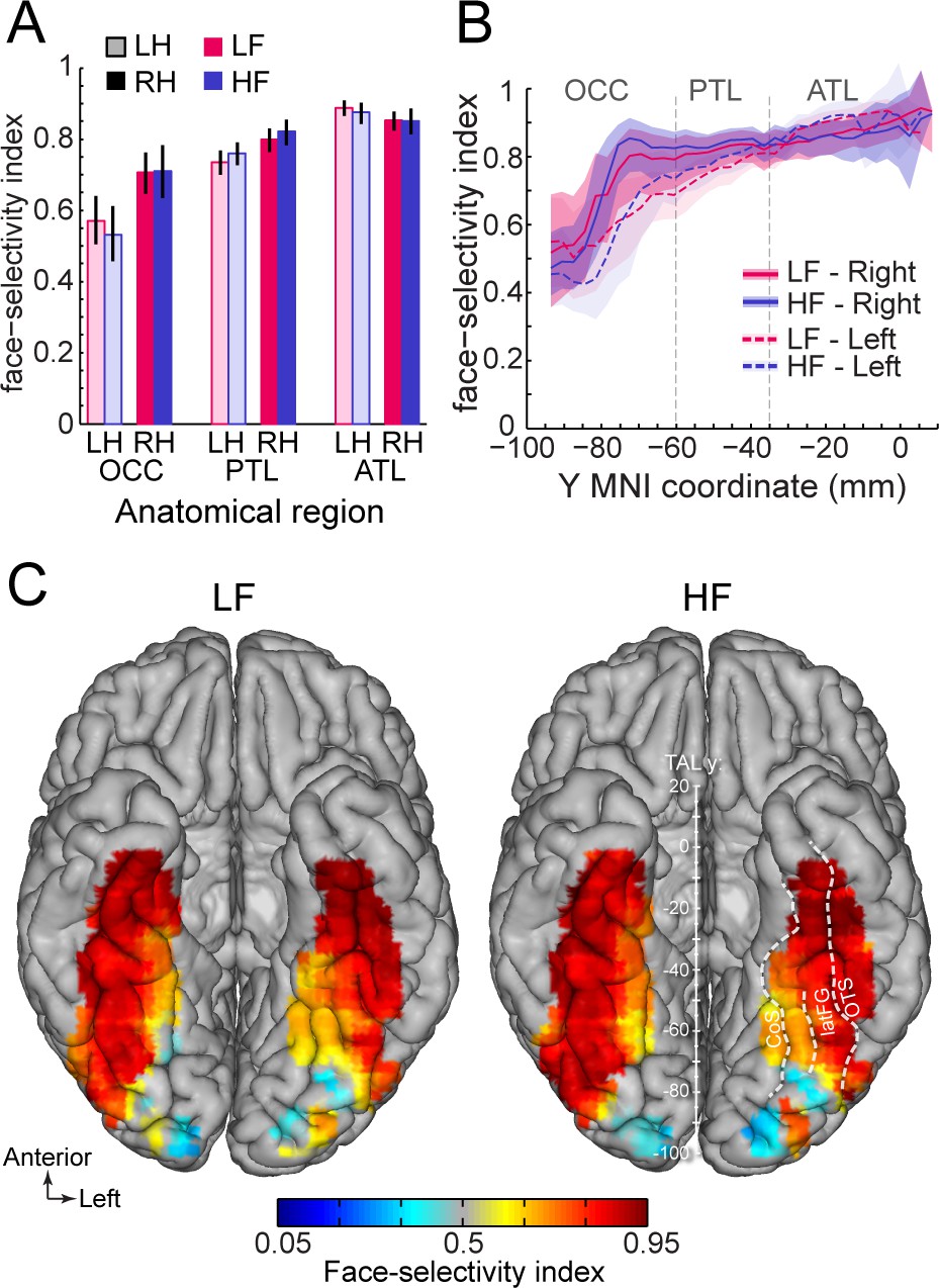
Similar face selectivity index for LF and HF.
(A) Face-selectivity index (FSI) for LF and HF signals computed over LF+HF+ contacts separately for each main region and hemisphere (light color = left hemisphere). Error bars are 99% confidence interval computed using a percentile bootstrap. (B) FSI along the antero-posterior axis for LF and HF. FSI is computed in each hemisphere collapsed along the X dimension (medio-lateral). The shaded area shows the 99% confidence interval. Approximate location of subdivision between main VOTC regions in the Talairach space are shown as dashed vertical lines. (C) VOTC maps of FSI for LF and HF responses computed over LF+HF+ contacts in 12x12 mm voxels in Talairach space.
Figure 8
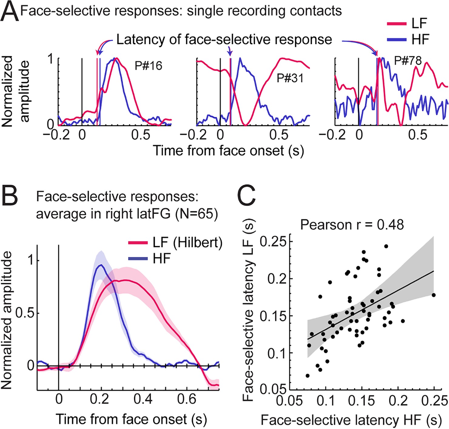
LF and HF timing relationship in the right latFG.
(A) Mean time-domain face-selective responses for LF and HF in three example recording contacts (from three different participants) with high (left, middle) or middle/low (right) face-selective Z-scores. LF and HF time-domain signals in FPVS sequences were segmented relative to each face onset (i.e. every 0.835 s). The signal related to the general visual response at 6 Hz and harmonics was selectively filtered-out, and resulting segments were averaged. Due to normalization (between 0 and 1 for display purpose), responses of differing polarity across signals result in misaligned pre-face-onset levels (e.g. middle plot, –0.166–0 s). Vertical lines show estimated onset latency of face-selective responses for LF and HF. (B) Time-domain face-selective responses averaged across 65 LF+HF+ recording contacts in the right latFG. The shaded area shows the standard error of the mean across contacts. For LF, to limit the influence of variation in response morphology or polarity across recording contacts, a Hilbert transform was applied to the response of each contact before averaging. Averaged time-domain responses were then normalized (0–1) and aligned for their pre-face-onset amplitude level (−0.166–0 s). (C) Scatter plot showing the relationship between the onset latency of LF and HF face-selective responses measured in individual recording contacts in the right latFG (see vertical lines in panel A). The shaded area shows the 99% confidence interval of the linear regression line computed by resampling data points with replacement 1000 times.
Tables
Table 1
Number of contacts showing significant responses in LF (LF+) and HFB (HFB+) in each anatomical region.
The corresponding number of participants in which these contacts were found is indicated in parenthesis. For each region, the larger anatomical subdivision is indicated in parenthesis. Acronyms: VMO: ventro-medial occipital cortex; IOG: inferior occipital gyrus; PHG: Parahippocampal Gyrus; medFG: medial fusiform gyrus and collateral sulcus; latFG: lateral FG and occipito-temporal sulcus; MTG/ITG: the inferior and middle temporal gyri; antPHG: anterior PHG; antCoS: anterior collateral sulcus; antOTS: anterior OTS; antFG: anterior FG; antMTG/ITG: anterior MTG and ITG; AMG: amygdala; HIP: hippocampus; TP: temporal pole; OCC: occipital lobe; PTL: posterior temporal lobe; ATL: anterior temporal lobe; MTL: Medial temporal lobe.
| Region | LF+ | HF+ | ||
|---|---|---|---|---|
| LH | RH | LH | RH | |
| VMO (OCC) | 104 (16) | 66 (10) | 35 (13) | 23 (9) |
| IOG (OCC) | 65 (16) | 90 (16) | 29 (11) | 49 (14) |
| PHG (PTL) | 5 (3) | 2 (1) | 1 (1) | 0 (0) |
| MedFG (PTL) | 105 (33) | 81 (24) | 64 (28) | 47 (20) |
| LatFG (PTL) | 125 (40) | 105 (31) | 60 (24) | 66 (26) |
| MTG/ITG (PTL) | 44 (25) | 45 (22) | 7 (6) | 5 (2) |
| antPHG (ATL) | 5 (5) | 0 (0) | 0 (0) | 0 (0) |
| antCoS (ATL) | 168 (55) | 148 (52) | 25 (18) | 36 (23) |
| antFG (ATL) | 27 (19) | 27 (17) | 12 (11) | 8 (7) |
| antOTS (ATL) | 198 (66) | 211 (61) | 64 (32) | 58 (34) |
| antMTG/ITG (ATL) | 49 (30) | 114 (45) | 5 (5) | 8 (7) |
| TP (ATL) | 19 (11) | 41 (18) | 2 (2) | 1 (1) |
| AMG (MTL) | 52 (30) | 67 (27) | 6 (5) | 2 (2) |
| HIP (MTL) | 55 (28) | 62 (33) | 2 (2) | 4 (4) |
| Total | 1021 | 1059 | 312 | 307 |
Additional files
Download links
A two-part list of links to download the article, or parts of the article, in various formats.
Downloads (link to download the article as PDF)
Open citations (links to open the citations from this article in various online reference manager services)
Cite this article (links to download the citations from this article in formats compatible with various reference manager tools)
Low and high frequency intracranial neural signals match in the human associative cortex
eLife 11:e76544.
https://doi.org/10.7554/eLife.76544


