Population-based sequencing of Mycobacterium tuberculosis reveals how current population dynamics are shaped by past epidemics
- Tuberculosis Genomics Unit, Instituto de Biomedicina de Valencia (IBV-CSIC), Spain
- Unidad Mixta "Infección y Salud Pública" (FISABIO-CSISP), Spain
- Microbiology Service, Hospital Clínico Universitario, Spain
- Microbiology and Parasitology Service, Hospital Universitario de La Ribera, Spain
- Microbiology Service, Hospital Arnau de Vilanova, Spain
- Microbiology Service, Hospital Universitario Dr Peset, Spain
- Department of Mathematics, Faculty of Science, Simon Fraser University, Canada
- Microbiology Laboratory, Hospital Virgen de los Lirios, Spain
- Microbiology Service, Hospital de Denia, Spain
- Computational Genomics Department, Centro de Investigación Príncipe Felipe, Spain
- Microbiology Service, Hospital Universitari i Politècnic La Fe, Spain
- Microbiology Service, Hospital General Universitario de Valencia, Spain
- Microbiology Service, Hospital General Universitario de Alicante, Spain
- Microbiology Service, Hospital General Universitario de Castellón, Spain
- Microbiology Service, Hospital Lluís Alcanyis, Spain
- Microbiology Service, Hospital General Universitario de Elche, Spain
- Microbiology Service, Hospital Universitario de San Juan de Alicante, Spain
- Microbiology Service, Hospital de la Vega Baixa, Spain
- Subdirección General de Epidemiología y Vigilancia de la Salud y Sanidad Ambiental de Valencia (DGSP), Spain
- Microbiology Service, Hospital de Sagunto, Spain
- CIBER of Epidemiology and Public Health (CIBERESP), Spain
Figures
Figure 1

Genomic characterization of the study region.
(A) Phylogeny of 775 tuberculosis (TB) isolates collected during the years 2014 and 2016. Each ring represents genomic clusters detected by different single nucleotide polymorphism (SNP) thresholds (0, 5, and 12 SNPs). Mycobacterium canneti was used as an outgroup. (B) Clustering percentage, i.e. percentage of samples within clusters for different SNP thresholds. (C) Number of genomic clusters by different cluster sizes. A 12 SNP threshold was used as a standard. Cluster sizes of 8–11 samples were not detected. *Nomenclature proposed by Comas et al., 2013.
-
Figure 1—source data 1
Genomic cluster types; Spanish: clusters including only Spanish-born cases; foreign: clusters including only foreign-born cases; mix: clusters including Spanish and foreign-born cases.
Cluster ID; number of Spanish. Foreign and unknown origin cases and total cluster size are indicated.
- https://cdn.elifesciences.org/articles/76605/elife-76605-fig1-data1-v1.xlsx
Figure 2
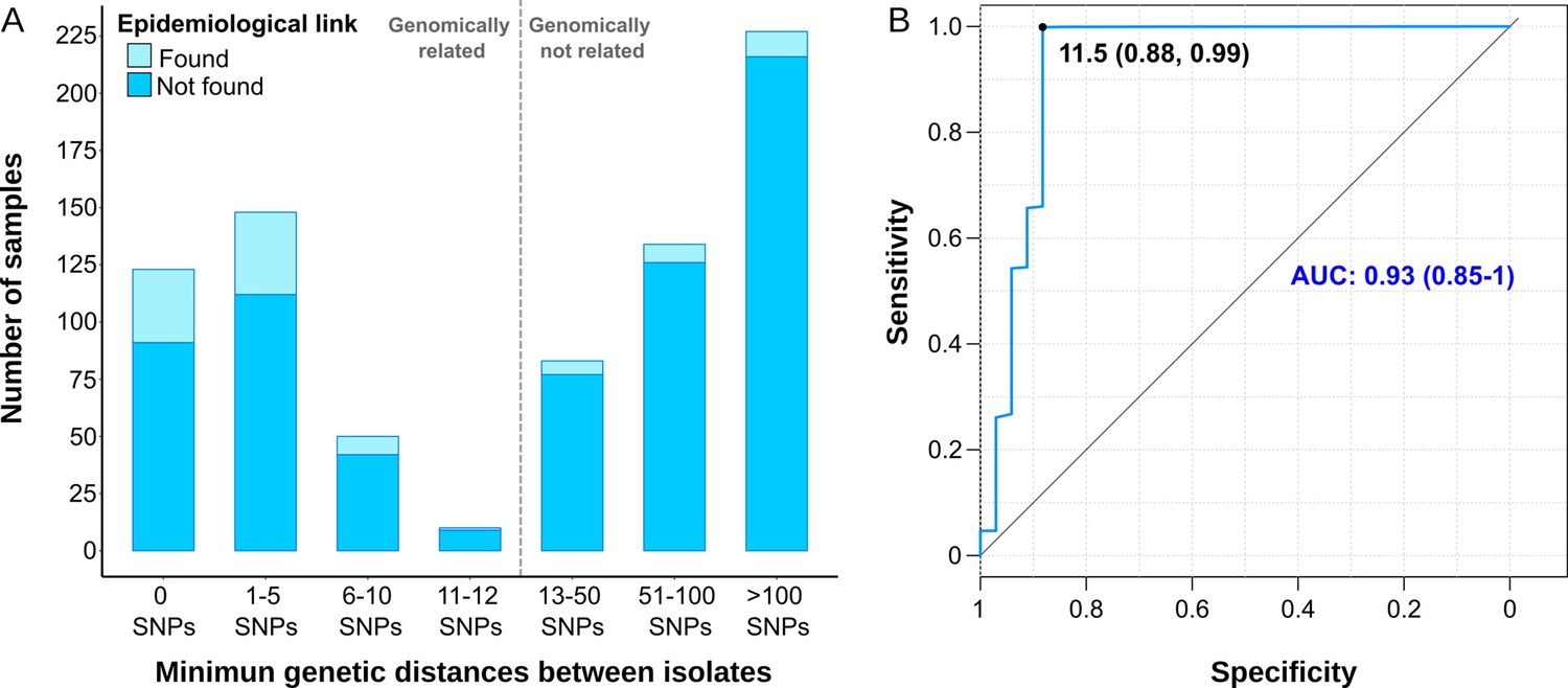
Comparison between epidemiological and genomic clustering.
(A) Clustered samples using different pairwise distance thresholds, bars denote the number of cases within clusters for each single nucleotide polymorphism (SNP) threshold. Gray dashed line separates the genomically linked samples (clustered) from those unlinked. (B) ROC (Receiver Operating Characteristics) curve for different pairwise distance thresholds between 0 and 2000 SNPs, indicating the optimal SNP cut-off values with its correspondent specificity and sensitivity values, the area under the curve (AUC), and its confidence intervals.
Figure 3 with 6 supplements

Historical transmission dynamics analysis.
(A) Distribution of local-born cases clustered by different pairwise distance SNP thresholds. Cases are expressed as the percentage of the plotted samples. Pie charts represent the proportion of local-born (color) and foreign-born (gray) cases in each dataset. (B) Age of local transmission links over time in each setting. Circles represent median time, and lines represent 95% high probability density for each transmission link counted. Circle size represents the number of samples included in the corresponding link. Red denotes those transmission links including only samples within the same genomic transmission clusters (gClusters), green denotes links involving samples from different gClusters, blue denotes samples within gClusters and unique, and purple denotes unique cases. All links were obtained from Figure 3—figure supplements 1–6 and are summarized in Figure 3—source data 1–6.
-
Figure 3—source data 1
Bayesian dating results for all clusters (CL) from Oxfordshire.
Data include information of cluster date (in years AD); cluster distances (min, max, mean, and median); most recent common ancestor (MRCA) time in years (AD) with corresponding 95% highest probability density (HPD) intervals and cluster time span or duration.
- https://cdn.elifesciences.org/articles/76605/elife-76605-fig3-data1-v1.xlsx
-
Figure 3—source data 2
Number of transmission links (TLs) traced back to 150 years before 2016 for Oxfordshire dataset.
Median time of all the local TLs pointed in Figure 3—figure supplement 1 were classified in different time windows. The total number of links within each time window is indicated even if they were links within a genomic cluster (total_CL) or not (total_noCL). Sampling period for Oxfordshire is 2007–2012.
- https://cdn.elifesciences.org/articles/76605/elife-76605-fig3-data2-v1.xlsx
-
Figure 3—source data 3
Bayesian dating results for all clusters (CL) from Valencia region.
Data include information of cluster date (in years AD); cluster distances (min, max, mean, and median); most recent common ancestor (MRCA) time in years (AD) with corresponding 95% highest probability density (HPD) intervals and cluster time span or duration.
- https://cdn.elifesciences.org/articles/76605/elife-76605-fig3-data3-v1.xlsx
-
Figure 3—source data 4
Number of transmission links (TLs) traced back to 150 years before 2016 for Oxfordshire dataset.
Median time of all the local TLs pointed in Figure 3—figure supplement 1 were classified in different time windows. The total number of links within each time window is indicated even if they were links within a genomic cluster (total_CL) or not (total_noCL). Sampling period for Oxfordshire is 2007–2012.
- https://cdn.elifesciences.org/articles/76605/elife-76605-fig3-data4-v1.xlsx
-
Figure 3—source data 5
Number of transmission links (TLs) traced back to 150 years before 2016 for Malawi dataset.
Analysis performed for Malawi. Median time of all the TLs pointed in Figure 3—figure supplement 2 were classified in different time windows. The total number of links within each time window is indicated even if they were links within a genomic cluster (total_CL) or not (total_noCL). Color code for links outside clusters (no_CL) are the same as in Figure 3—figure supplement 2. Sampling period for Malawi is 2008–2010.
- https://cdn.elifesciences.org/articles/76605/elife-76605-fig3-data5-v1.xlsx
-
Figure 3—source data 6
Number of transmission links (TLs) traced up to 150 years before 2016 for Valencia dataset.
Median time of all the TLs pointed in Figure 3—figure supplements 3–6 were classified in different time windows. The total number of links within each time window is indicated even if they were links within a genomic cluster (total_CL) or not (total_noCL). Color code for links outside clusters (no_CL) are the same as in Figure 3—figure supplements 3–6. Sampling period for Valencia is 20014–2016. The percentage of Spanish cases within each TL was evaluated in a global phylogeny as a proxi of the origin of the node.
- https://cdn.elifesciences.org/articles/76605/elife-76605-fig3-data6-v1.xlsx
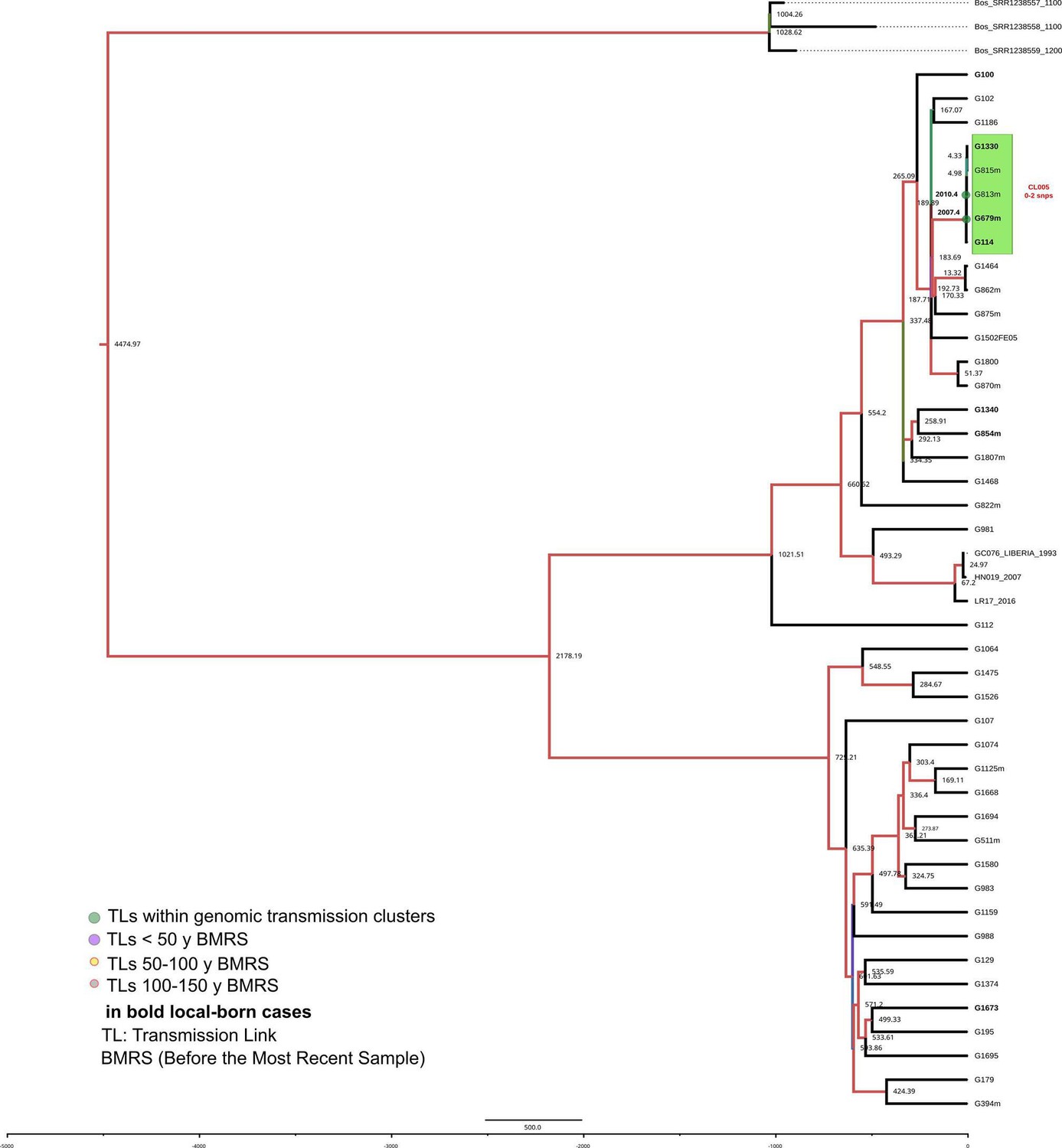
Figure 3—figure supplement 1
Bayesian time tree for Oxfordshire dataset.
Sample names in bold represent local born cases. Local clusters (CLs) are highlighted in orange and mixed CLs in green (those including foreign cases). The CL numbers are crossreferenced in Figure 3—source data 1. The transmission links’ (TLs’) dates used in the analysis are indicated in bold and expressed as AD, the other TLs’ dates are indicated as years before 2016 AD. Branch colors represent Bayesian posterior values being red the highest posterior, blue median, and green the lowest values. Numbers in TLs nodes are crossreferenced in Figure 3—source data 4.
Figure 3—figure supplement 2
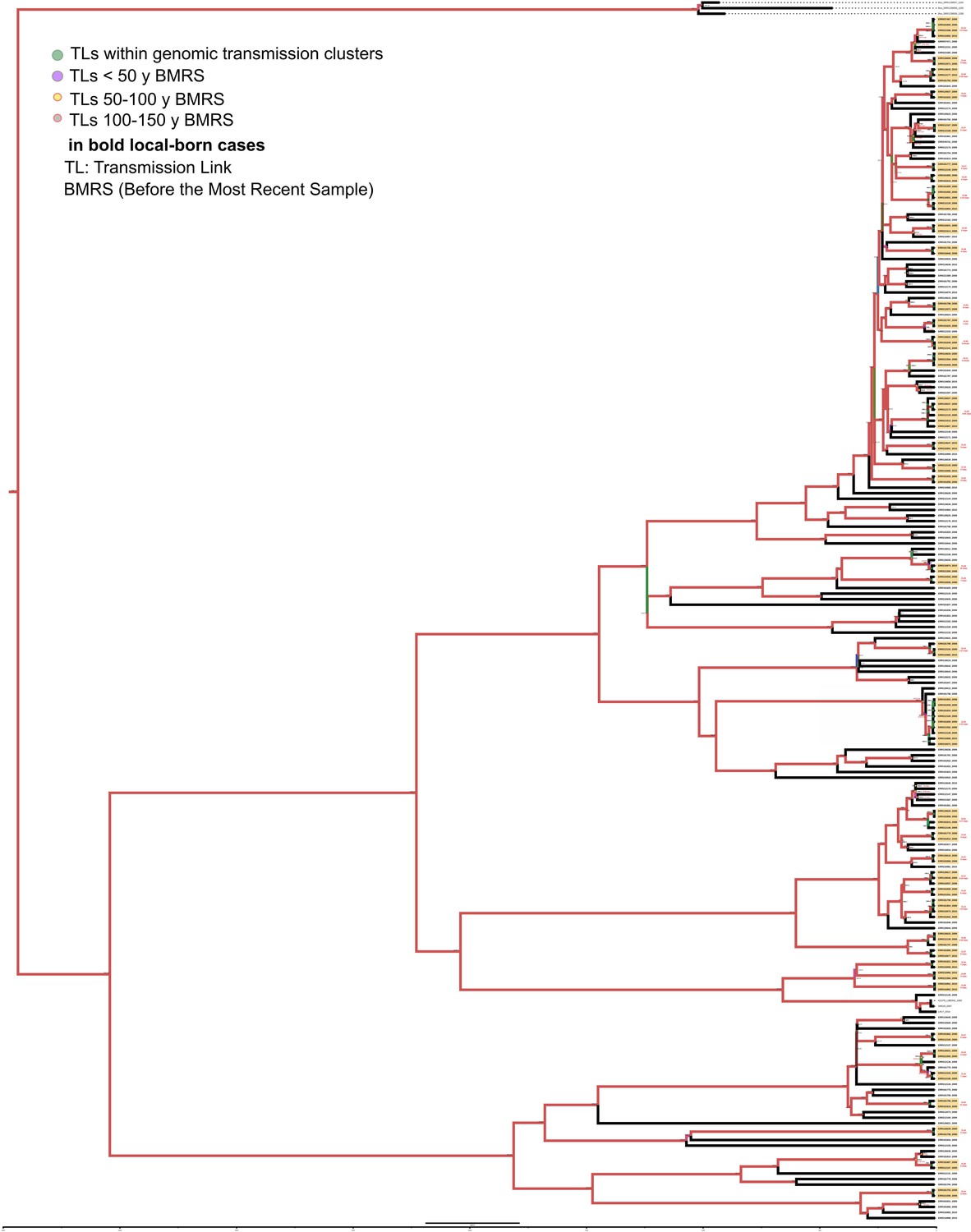
Bayesian time tree for Malawi dataset.
Sample names in bold represent local born cases. Local clusters (CLs) are highlighted in orange and mixed CLs in green (those including foreign cases). The CL numbers are crossreferenced in Figure 3—source data 2. The transmission links’ (TLs’) dates used in the analysis are indicated in bold and expressed as AD, the other TLs’ dates are indicated as years before 2016 AD. Branch colors represent Bayesian posterior values being red the highest posterior, blue median, and green the lowest values. Numbers in TLs nodes are crossreferenced in Figure 3—source data 5.
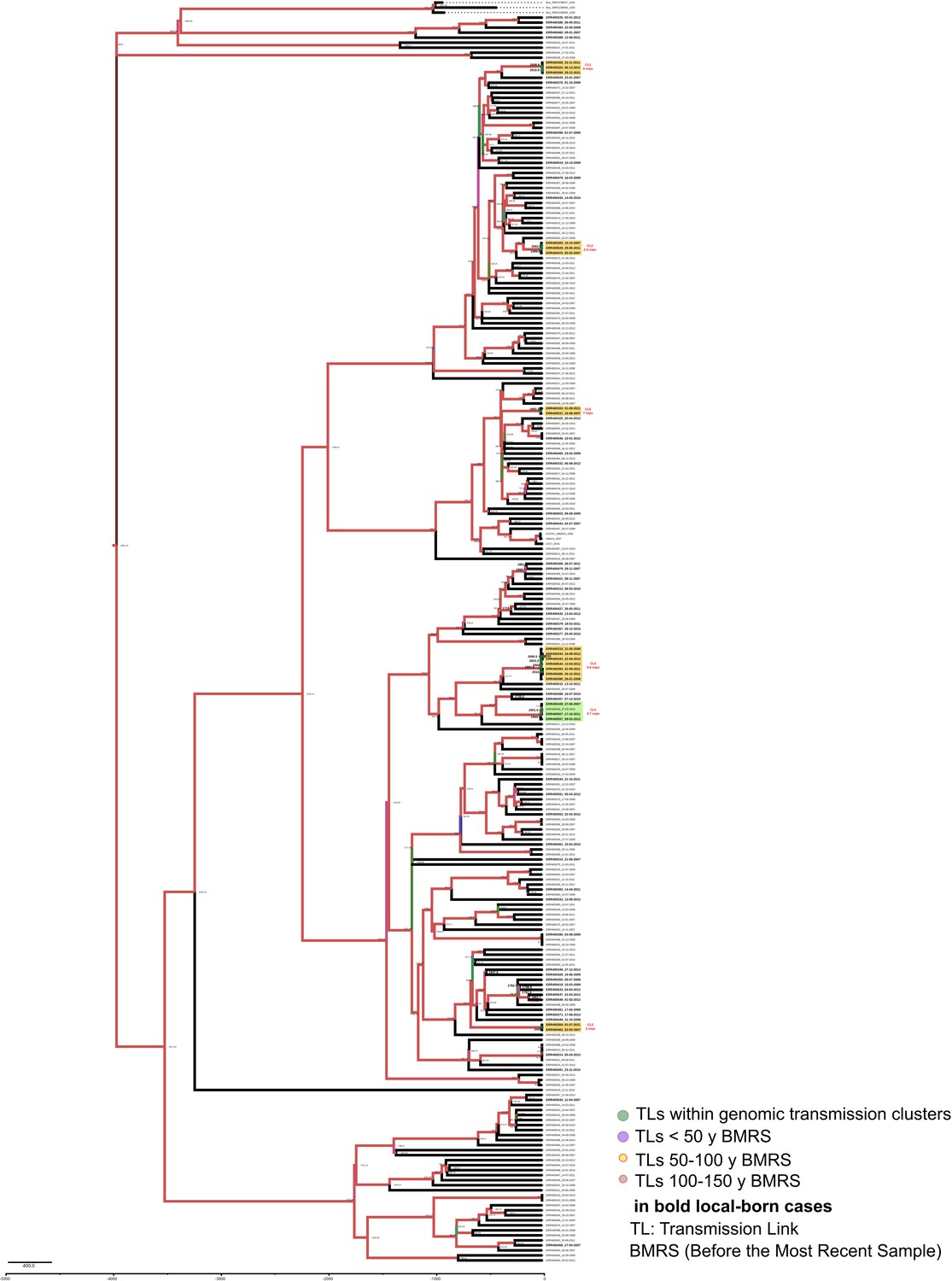
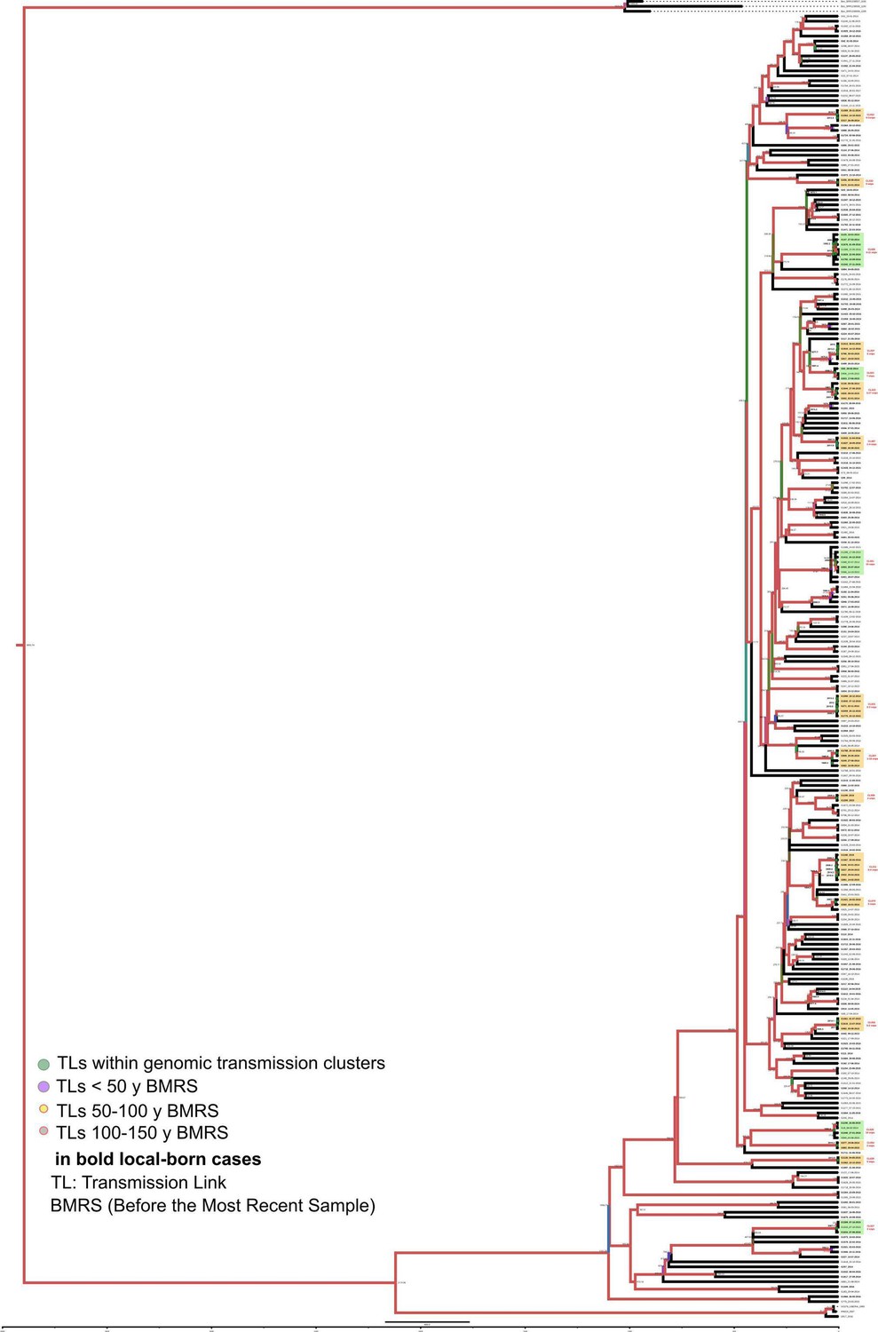
Figure 3—figure supplement 3
Bayesian time tree for Valencia region dataset.
Sample names in bold represent local born cases. Local clusters (CL) are highlighted in orange and mixed CL in green (those including foreign cases). The CL numbers are crossreferenced in Figure 3—source data 3. The transmission links’ (TLs’) dates used in the analysis are indicated in bold and expressed as AD, the other TLs’ dates are indicated as years before 2016 AD. Branch colors represent Bayesian posterior values being red the highest posterior, blue median and green the lowest values. Numbers in TLs nodes are crossreferenced in Figure 3—source data 6.
Figure 3—figure supplement 4
Bayesian time tree for Velncia Region dataset.
Sample names in bold represent local born cases. Local clusters are highlighted in orange and mixed clusters in green (those including foreign cases). CL numbers are crossreferencied in Figure 3—source data 3. TLs’ dates used in the analysis are indicated in bold and expressed as AD, the other TLs’ dates are indicated as years before 2016 AD. Branch colors represent bayesian posterior values being red the highest posterior, blue median and green the lowest values. Numbers in TLs nodes are cross referencend in Figure 3—source data 6.
Figure 3—figure supplement 5

Bayesian time tree for Valencia Region dataset.
Sample names in bold represent local born cases. Local clusters are highlighted in orange and mixed clusters in green (those including foreign cases). CL numbers are crossreferencied in Figure 3—source data 3. TLs’ dates used in the analysis are indicated in bold and expressed as AD, the other TLs’ dates are indicated as years before 2016 AD. Branch colors represent bayesian posterior values being red the highest posterior, blue median and green the lowest values. Numbers in TLs nodes are crossreferencend in Figure 3—source data 6.
Figure 3—figure supplement 6

Bayesian time tree for Valencia Region dataset.
Sample names in bold represent local born cases. Local clusters are highlighted in orange and mixed clusters in green (those including foreign cases). CL numbers are crossreferencied in Figure 3-source data 3. TLs’ dates used in the analysis are indicated in bold and expressed as AD, the other TLs’ dates are indicated as years before 2016 AD. Branch colors represent bayesian posterior values being red the highest posterior, blue median and green the lowest values. Numbers in TLs nodes are crossreferencend in Figure 3—source data 6.
Figure 4
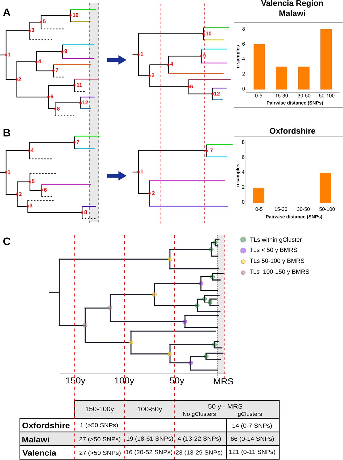
Hypothetical time trees indicating transmission links (TLs).
(A) (Left) The complete phylogeny, including all bacterial isolates and displaying multiple transmission events over time (located at nodes for simplification). This scenario allows the reconstruction of a tree (middle) with several tips and multiple TLs (as the summary of all the events). A continuous distribution of clustered cases by different pairwise distances is retrieved (right) as observed in the Valencia region and Malawi. (B) A complete phylogeny (left) in which transmission is either too old or recent and few (or no) transmission events occurred in the middle time, led to the reconstruction of a tree (middle) in which few samples reach the present and fewer nodes are observed all over the tree. This scenario provides a bimodal distribution of clustered cases by pairwise distance (right) as observed for Oxfordshire. (C) Time tree highlighting TLs over time before the most recent sample (BMRS). The table (bottom) shows the number of links counted in each time period and the median distance range among the samples within the links for the three settings analyzed. For the period between the most recent sample (MRS) and 50 y BMRS, links within (gClusters) and outside gClusters (No gClusters) are indicated. Vertical red lines indicate periods of time, horizontal dashed lines indicate missing samples, shaded areas indicate sampling period, and circles indicate transmission events with colors specified in the legend.
Appendix 1—figure 1
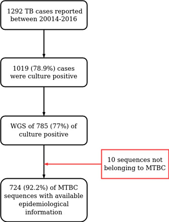
Workflow for sample selection.
MTBC, Mycobacterium tuberculosis complex; WGS, whole genome sequencing.
Appendix 1—figure 2
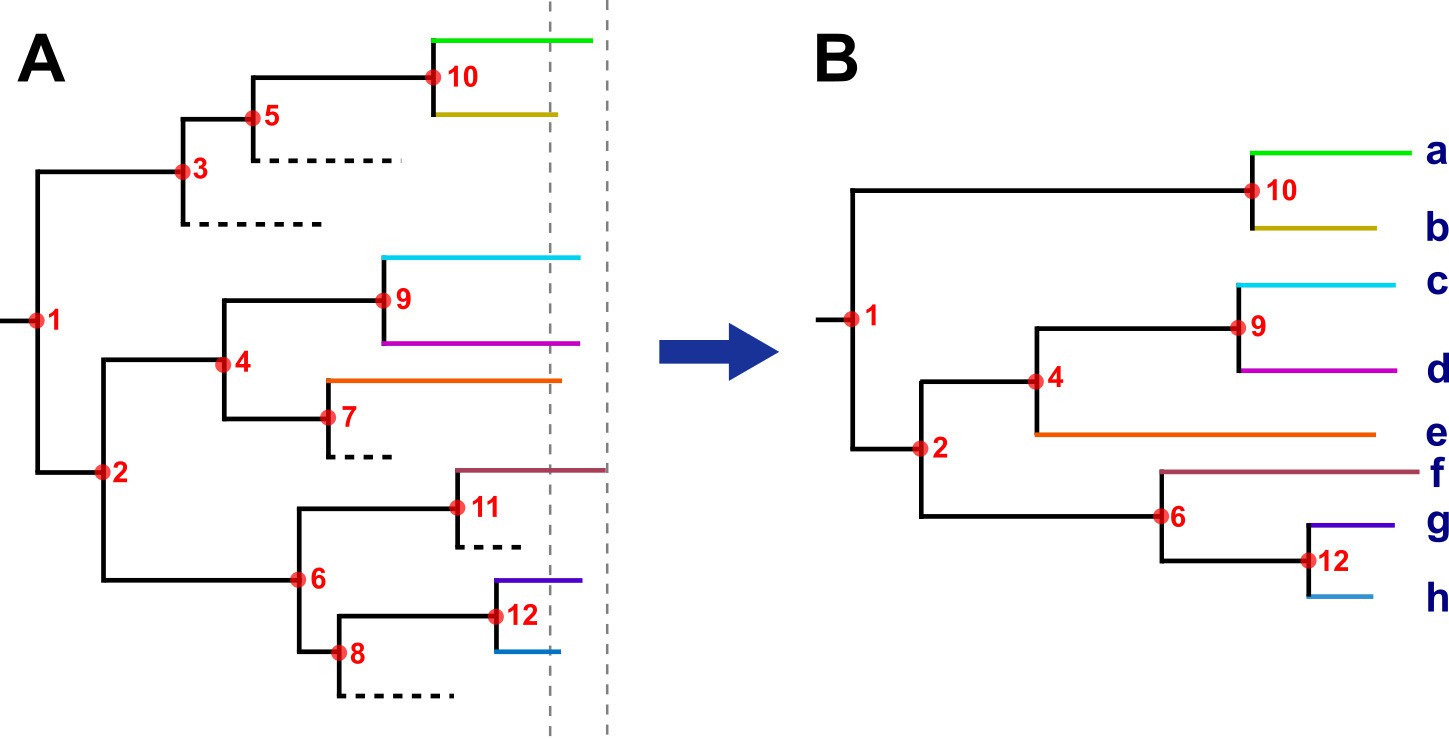
Hypothetical time tree.
(A) Complete phylogeny, including all bacterial isolates. Dashed lines represent missing samples that could not be retrieved during the sampling period (gray dashed lines). Transmission events are indicated as red circles, always in the tree node for simplification; multiple events occurred widely distributed across time phylogeny. (B) The tree was reconstructed with the collected samples. Most, but not all, transmission events can be recovered, they were summarized as ‘transmission links’. Letters indicate samples collected.
Appendix 1—figure 3
Boxplots of ages of cases from spanish-born genomic clusters in the Valencia region vs. the inferred ancestor of the clusters.
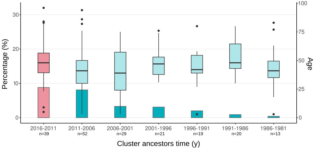
Bars represent the percentage of cases in gClusters (by 12 SNPs) for each time period. Boxplots represent the age distribution of patients within the clusters. Differences between the age cases for each time period against the most recent clusters (pink) are not significant (Welch two-samples t-test, p-value < 0.1 detailed in Supplementary file 7). Sample size of each category is indicated in x-axis label.
Appendix 1—figure 4
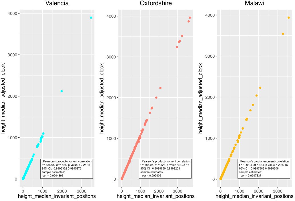
Correlation between the height median estimated by two ascertainment bias correction approaches; ‘adjusting clock rate’ and ‘including invariant positions’.
Correlation was calculated for each dataset.
Author response image 1
Author response image 2
Tables
Table 1
Dating of local genomic clusters (gCluster).
Times of the oldest and youngest local gClusters obtained by a Bayesian analysis are presented, with values in years (AD) and 95% highest posterior density given in brackets. The number of gClusters and clustering percentage is provided for each dataset. The median distance ranges for all gClusters are also detailed.
| Dataset | Sampling period | Local samples | N local gCluster | Local clustering | Median distance range | Oldest gCluster | Youngest gCluster |
|---|---|---|---|---|---|---|---|
| Oxfordshire | 2006–2012 | 74 | 6 | 27% | 0–7 | 1993 (1982–2003) | 2009 (2003–2012) |
| Malawi | 2008–2010 | 106 | 40 | 49.80% | 0–14 | 1979 (1968–1988) | 2009 (2004–2010) |
| Valencia region | 2014–2016 | 456 | 65 | 47.40% | 0–11 | 1985 (1972–1996) | 2015 (2012–2016) |
Author response table 1
Total cases expected: 3 cases, cases observed: 5*based on (Chaoui et al., 2014; Coscolla et al., 2021; de Jong et al., 2010; Gehre et al., 2016; Yeboah-Manu et al., 2017).
| Origen | #total_patients | %_reported* | cases_expected |
|---|---|---|---|
| MAURITANIA | 1 | no data | |
| SENEGAL | 7 | 20 | 1.4 |
| GUINEA EQ | 6 | no data | |
| CAMEROON | 1 | 12 | 0.12 |
| MALI | 4 | 20 | 0.8 |
| NIGERIA | 2 | 11 | 0.2 |
| MOROCCO | 47 | no Africanum reported | |
| IVORY | 1 | 22 | 0.2 |
| ALGERIA | 5 | no data |
Additional files
-
Supplementary file 1
Samples included in this study and all clinical.
Laboratory and epidemiological data associated. WGS data includes all the information obtained by WGS; run accession number are included in the ENA projects PRJEB29604 and PRJEB38719; depth coverage. MTBC lineage. genomic and epidemiological clusters ID. Patient information including: age, gender, country of birth, year of arrival to Spain, and province of residence in the Valencia region. NA indicates not available epidemiological information.
- https://cdn.elifesciences.org/articles/76605/elife-76605-supp1-v1.xlsx
-
Supplementary file 2
Beast input file (.xml) indicating ascertainment bias correction implemented.
- https://cdn.elifesciences.org/articles/76605/elife-76605-supp2-v1.zip
-
Supplementary file 3
Demographic.
clinical and epidemiological data for all culture positive cases and sequenced samples reported between 2014 and 2016 in Valencia region.
- https://cdn.elifesciences.org/articles/76605/elife-76605-supp3-v1.xlsx
-
Supplementary file 4
Statistical analysis of clustered vs. unique TB cases.
Age, sex, place of birth, sputum smear, and disease type were considered in the analysis for all TB cases and for Spanish-born only.
- https://cdn.elifesciences.org/articles/76605/elife-76605-supp4-v1.xlsx
-
Supplementary file 5
Epidemiological cluster evaluation.
Clusters identified by epidemiological links were compared against genomic clustering. Similarities and discrepancies between both methods are described for all samples. Cluster size and pairwise distance among the samples included in the cluster are mentioned. Median time and 95% HPD (highest posterior density) of the most common ancestor (tMRCA) for the cluster obtained by both approaches are provided. For mean and median values. Only the clusters with tMRCA were considered.
- https://cdn.elifesciences.org/articles/76605/elife-76605-supp5-v1.xlsx
-
Supplementary file 6
Performance of the WGS method for transmission.
Values were extracted from 724 clinical TB isolates and assumed epidemiological links from contact tracing as the gold standard. NPV, negative predictive value; PPV, positive predictive value.
- https://cdn.elifesciences.org/articles/76605/elife-76605-supp6-v1.xlsx
-
Supplementary file 7
Patients mean age for those cases within genomic clusters which ancestors’ age are included in different time windows in Valencia region.
- https://cdn.elifesciences.org/articles/76605/elife-76605-supp7-v1.xlsx
-
MDAR checklist
- https://cdn.elifesciences.org/articles/76605/elife-76605-mdarchecklist1-v1.pdf
Download links
A two-part list of links to download the article, or parts of the article, in various formats.
Downloads (link to download the article as PDF)
Open citations (links to open the citations from this article in various online reference manager services)
Cite this article (links to download the citations from this article in formats compatible with various reference manager tools)
Population-based sequencing of Mycobacterium tuberculosis reveals how current population dynamics are shaped by past epidemics
eLife 11:e76605.
https://doi.org/10.7554/eLife.76605


