Putting perception into action with inverse optimal control for continuous psychophysics
- Centre for Cognitive Science, Technical University of Darmstadt, Germany
- Institute of Psychology, Technical University of Darmstadt, Germany
- Frankfurt Institute for Advanced Studies, Goethe University Frankfurt, Germany
Figures
Figure 1
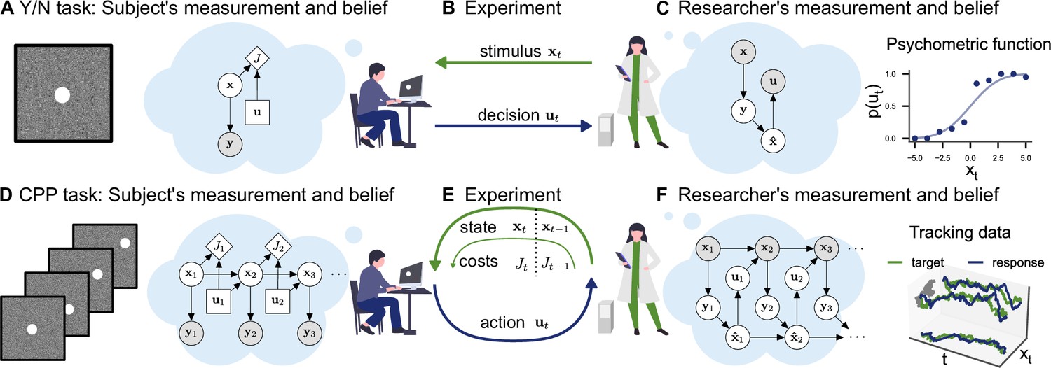
Conceptual frameworks for classical and continuous psychophysics.
(A) In a classical psychophysics task, the subject receives stimuli xt on independent trials, generates sensory observations yt, forms beliefs about the stimulus , and (B) makes a single decision ut (e.g., whether the target stimulus was present or absent). (C) The researcher has a model of how the agent makes decisions and measures the subject’s sensitivity and decision criterion by inverting this model. For example, one can estimate the agent’s visual uncertainty by computing the width of a psychometric function. (D) In a continuous psychophysics task, a continuous stream of stimuli is presented. The subject has an internal model of the dynamics of the task, which they use to form a belief about the state of the world and then perform continuously actions (E) based on their belief and subjective costs. (F) The researcher observes the subject’s behavior and inverts this internal model, fo example, using Bayesian inference applied to optimal control under uncertainty.
Figure 2 with 1 supplement
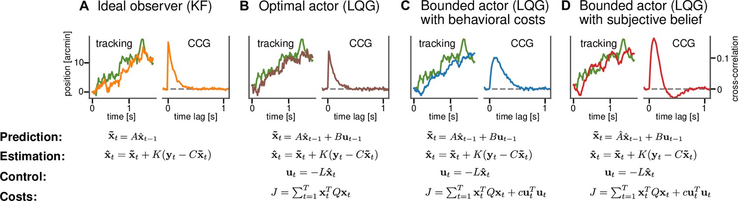
Computational models for continuous psychophysics.
(A) In the Kalman filter (KF) model, the subject makes an observation with Gaussian variability at each time step. They combine their prediction with their observation to compute an optimal estimate . (B) In the optimal control models, this estimate is then used to compute an optimal action using the linear quadratic regulator (LQR). The optimal action can be based on the task goal only or (C) bounded by internal costs, which, for example, penalize large movements. (D) Finally, the subject may act rationally using optimal estimation and control, but may use a subjective internal model of stimulus dynamics that differs from the true generative model of the task. These four different models are illustrated with an example stimulus and tracking trajectory (left subplots) and corresponding cross-correlograms (CCG, right subplots; see Mulligan et al., 2013 and ‘Cross-correlograms’).
Figure 2—figure supplement 1

Pareto efficiency plot.
The Pareto efficiency plot visualizes the trade-off between two costs contributing to the cost function. The cost function is composed of two terms: state costs and action costs , whose importance is balanced by the control cost parameter c. In a simulation, we computed these two terms separately for different values of c (see color bar) and plot them against each other. We did this for two levels each of action variability () and perceptual uncertainty (σ). First, there is a trade-off between tracking the target (state costs) and expending control effort (action costs): the better you track the target, the more action costs you have to tolerate. Second, the tracking performance depends on the values of the other two parameters: For a specific level of action variability and perceptual uncertainty σ, there is a minimum level of state costs incurred, which cannot be alleviated by decreasing action costs via c.
Figure 3 with 1 supplement
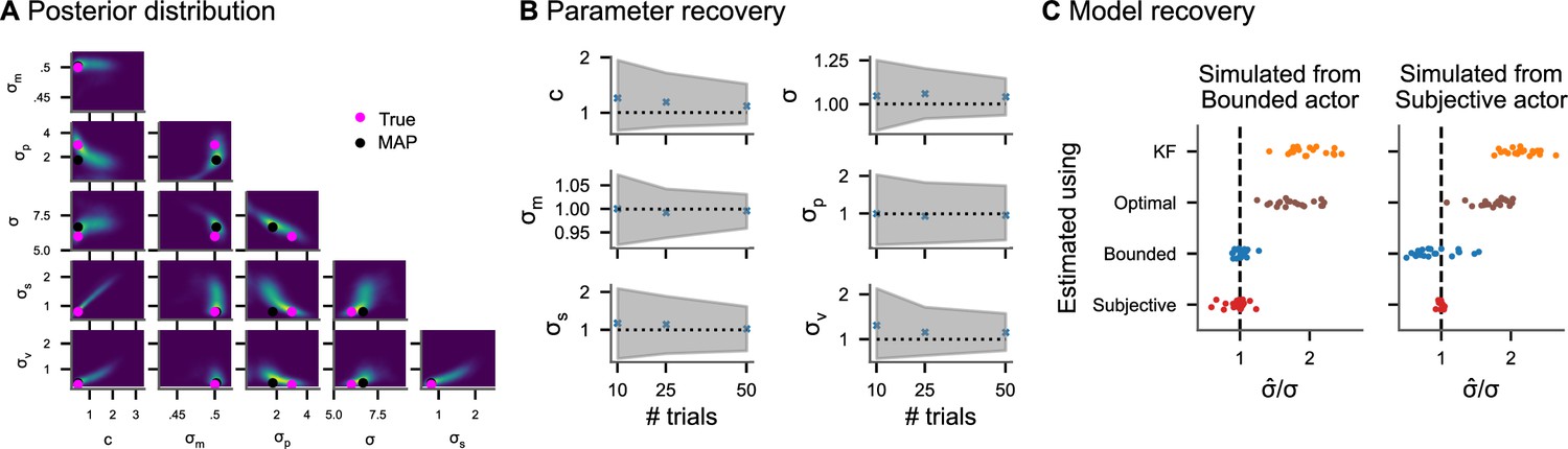
Inference on simulated data.
(A) Pairwise joint posterior distributions (0.5, 0.9, and 0.99 highest density intervals) inferred from simulated data from the subjective actor with parameters representative of real tracking data (, , , , , and ). The pink dots mark the true value used to simulate the data, while the black dots mark the posterior mode. (B) Average posterior means and average 95% credible intervals relative to the true value for different numbers of trials (200 repetitions each). (C) Model recovery analysis. Inferring perceptual uncertainty (, posterior mean relative to the true value) with each of the four models from data simulated from the bounded actor model and subjective actor model, respectively.
Figure 3—figure supplement 1

Model comparison for simulations.
Model comparison using widely applicable information criterion (WAIC) between different models fit to data simulated from the bounded actor or subjective actor model. Error bars indicate 95% CIs across 20 simulated datasets.
Figure 4
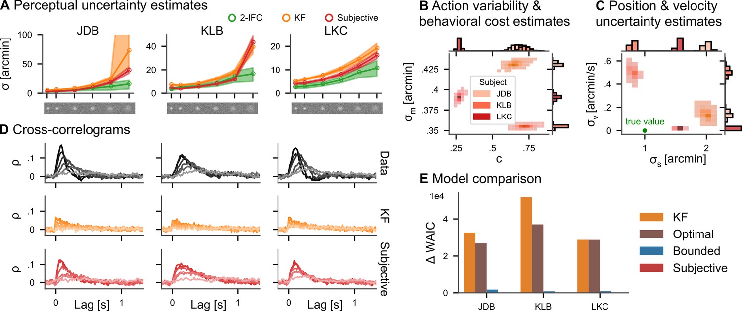
Continuous psychophysics.
(A) Perceptual uncertainty (σ) parameter estimates (posterior means) for the two-interval forced-choice (2IFC) task and the tracking task (Kalman filter [KF] and linear quadratic Gaussian [LQG] models) in the six blob width conditions (Bonnen et al., 2015). The shaded area represents 95% posterior credible intervals. (B) Posterior distributions for action cost () and action variability (). (C) Posterior distributions for subjective stimulus dynamics parameters (position: , velocity: ). The true values of the target’s random walk are marked by a green point. (D) Cross-correlograms (CCGs) of the empirical data and both models for all three subjects. (E) Model comparison. The difference in widely applicable information criterion (WAIC) w.r.t. the best model is shown with error bars representing WAIC standard error. Models without control cost (KF and optimal) fare worst, while the subjective model has the highest predictive accuracy.
Figure 5 with 2 supplements
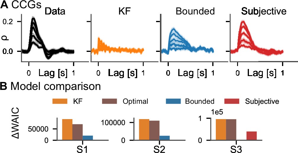
Model comparison on motion-tracking data.
(A) Average cross-correlograms (CCGs) for S1 from Bonnen et al., 2017 and three models in different target random walk conditions. For the other two subjects, see Figure 3. (B) Difference in widely applicable information criterion (WAIC) w.r.t. best model.
Figure 5—figure supplement 1

Cross-correlograms (CCGs) for all subjects.
(A) CCGs as in Figure 5 for all three subjects separately based on the data in experiment 2 from Bonnen et al., 2017.
Figure 5—figure supplement 2
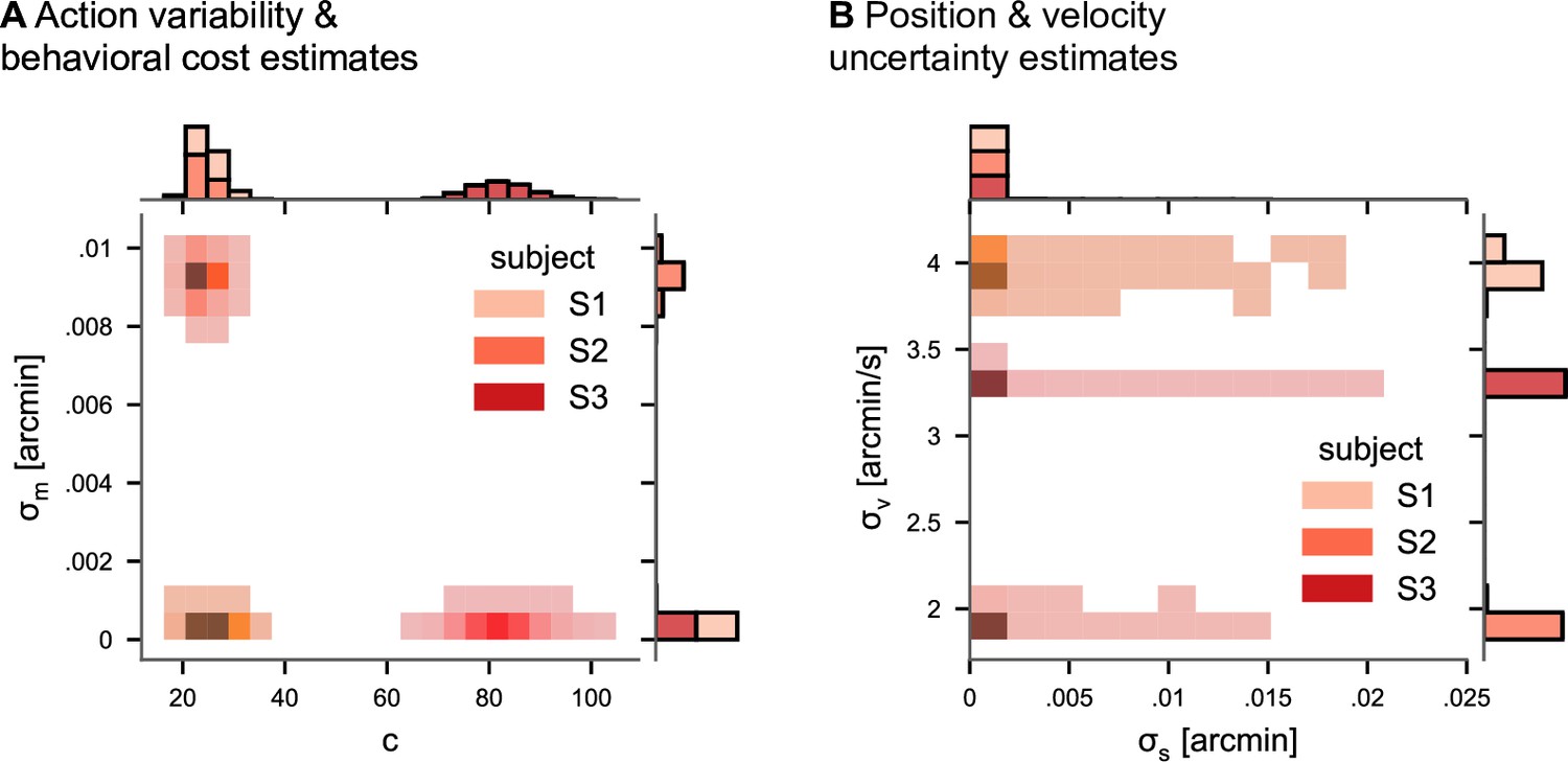
Posterior distributions of model parameters of the subjective model in experiment 2 (Bonnen et al., 2017).
(A) Posterior distributions for action cost (c) and action variability (). (B) Posterior distributions for subjective stimulus dynamics parameters (position: , velocity: ).
Appendix 5—figure 1
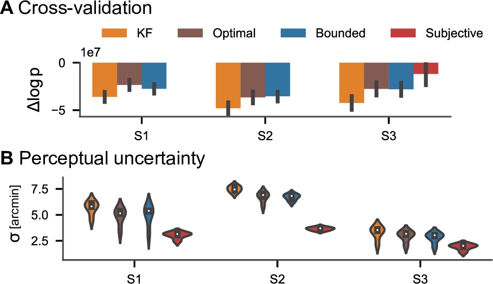
Cross-validation of estimated parameters.
(A) Difference in log-posterior relative to the best model per left-out condition from the experiment by Bonnen et al., 2017. Each model was fitted on the remaining four conditions as described in Appendix 5. In all but one condition of one participant, the model with a subjective component accounts best for the data. Error bars indicate 95% CIs across the 5 cross-validation runs. (B) Perceptual uncertainty (posterior mean) estimates across cross-validation conditions.
Appendix 5—figure 2
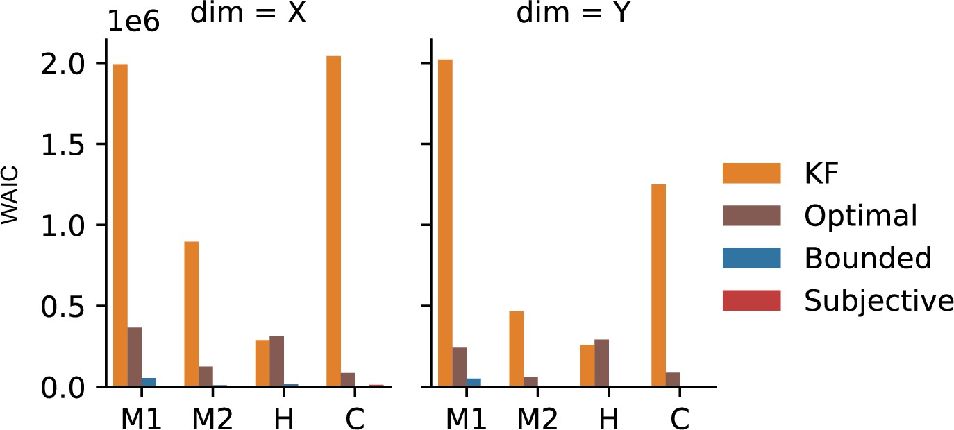
Model comparison on eye-tracking data.
Widely applicable information criterion (WAIC) on our four models for the eye-tracking data, fit separately to the X and Y dimension.
Tables
Appendix 2—table 1
Model overview.
| Model | State space | Dynamical systemmatrices | Cost function | Free parameters |
|---|---|---|---|---|
| Ideal observer | - | σ | ||
| Optimal actor | ||||
| Bounded actor | as above as above | as above as above | as above, as above | |
| Subjective actor |
Additional files
Download links
A two-part list of links to download the article, or parts of the article, in various formats.
Downloads (link to download the article as PDF)
Open citations (links to open the citations from this article in various online reference manager services)
Cite this article (links to download the citations from this article in formats compatible with various reference manager tools)
Putting perception into action with inverse optimal control for continuous psychophysics
eLife 11:e76635.
https://doi.org/10.7554/eLife.76635


