Figures and data in Cells use molecular working memory to navigate in changing chemoattractant fields

Version of Record

Accepted for publication after peer review and revision.

Download
Cite
Share
CommentOpen annotations (there are currently 0 annotations on this page).

Version of Record published: July 14, 2022 (This version)
Accepted Manuscript published: June 6, 2022 (Go to version)
Accepted: June 3, 2022
Received: January 6, 2022
Preprint posted: November 12, 2021 (Go to version)

Figures
Tables
Additional files

9 figures, 1 table and 2 additional files

Figures

Figure 1 with 2 supplements

Download asset Open asset

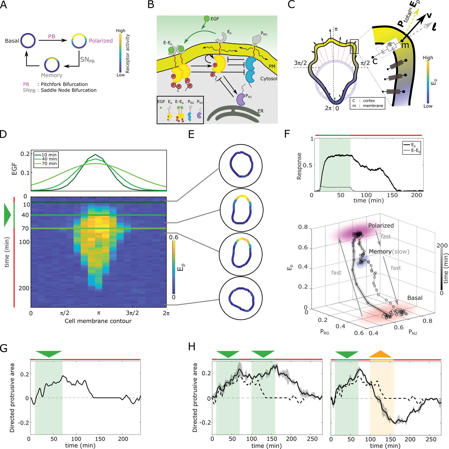
In silico manifestation of metastable polarized membrane signaling, as a mechanism for sensing changing spatial-temporal signals.

(A) Dynamical mechanism: sub-critical pitchfork bifurcation ( $P B$ ) determines stimulus-induced transition (arrow) between basal unpolarized and polarized receptor signaling state, whereas the associated saddle-node through which the $P B$ is stabilized ( $S N_{P B}$ ) gives rise to a ‘ghost’ memory state upon signal removal for organization at criticality (before the $S N_{P B}$ ). See Figure 1—figure supplement 1A and Methods for detailed description of these transitions. (B) Scheme of the EGFR-PTP interaction network. Ligandless EGFR ( $E_{p}$ ) interacts with PTPRG ( $P_{R G}$ ) and PTPN2 ( $P_{N 2}$ ). Liganded EGFR ( $E - E_{p}$ ) promotes autocatalysis of $E_{p}$ . Causal links - solid black lines; curved arrow lines - diffusion, PM - plasma membrane, ER- endoplasmic reticulum. See also Figure 1—figure supplement 1B. (C) Signal-induced shape-changes during cell polarization. Arrows: local edge velocity direction. Zoom: Viscoelastic model of the cell - parallel connection of an elastic and a viscous element. $P_{total}$ : total pressure; v: local membrane velocity; l: viscoelastic state. Bold letters: vectors. Cell membrane contour: $[0, 2 π]$ . (D) Top: In silico evolution of spatial EGF distribution. Bottom: Kymograph of $E_{p}$ for organization at criticality from reaction-diffusion simulations of the network in (B). Triangle - gradient duration. (E) Corresponding exemplary cell shapes with color coded $E_{p}$ , obtained with the model in (C). (F) Top: Temporal profiles $E_{p}$ (black) and $E - E_{p}$ (gray). Green shaded area: EGF gradient presence. Bottom: State-space trajectory of the system with denoted trapping state-space areas (colored) and respective time-scales. See also Figure 1—video 1. Thick/thin line: signal presence/absence. (G) Quantification of in silico cell morphological changes from the example in (E). Triangle - gradient duration. (H) Left: same as in (G), only when stimulated with two consecutive dynamic gradients (triangles) from same direction. Second gradient within the memory phase of the first. See also Figure 1—figure supplement 1D. Right: the second gradient (orange triangle) has opposite direction. See also Figure 1—figure supplement 1E. Dashed line: curve from (G). Mean ± s.d. from n=3 is shown. Parameters: Materials and methods. In (**D-H**), green(orange)/red lines: stimulus presence/absence.

Figure 1—figure supplement 1

Download asset Open asset

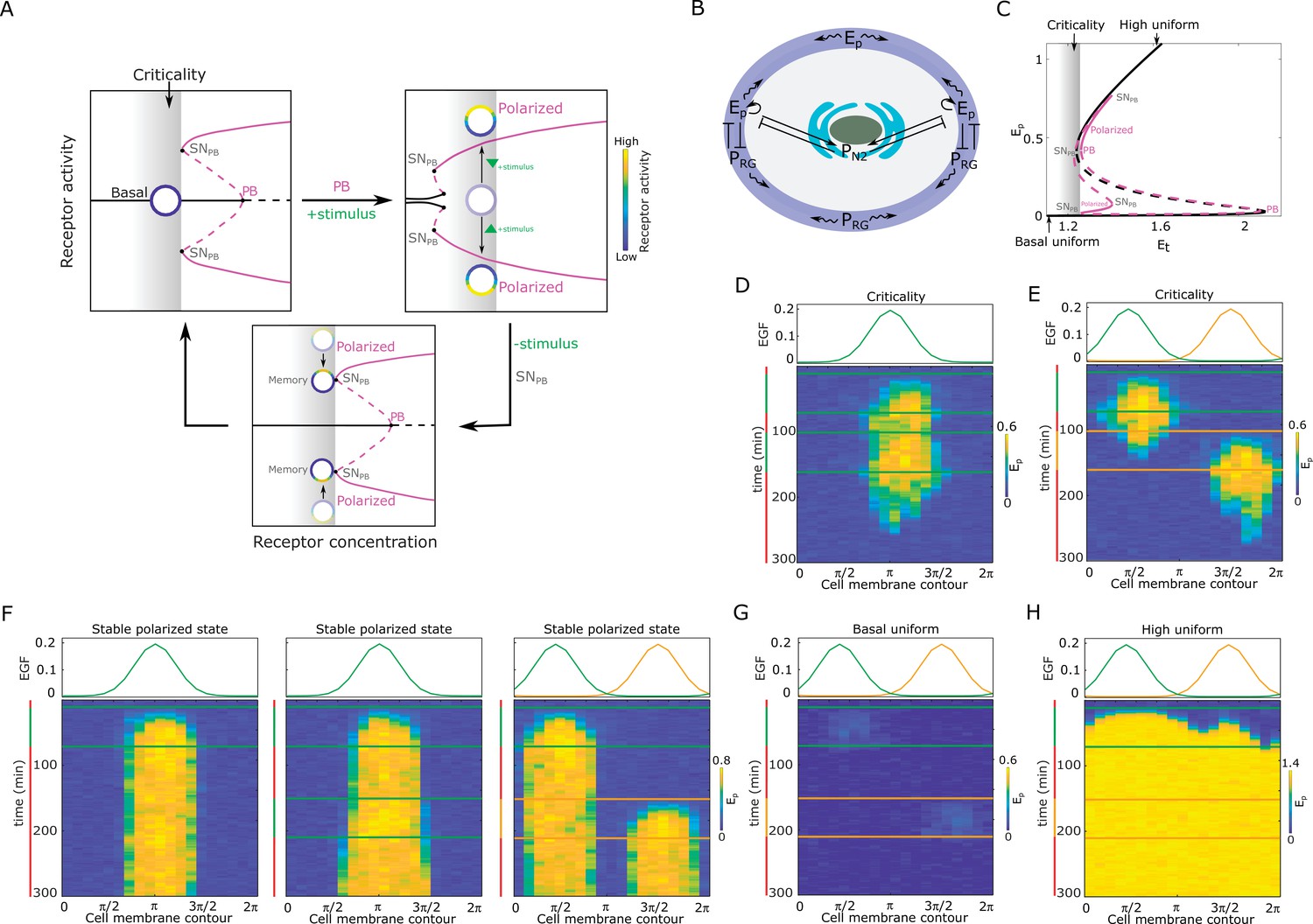
Features of receptor activity for different organization in parameter space.

(A) Dynamical mechanism of signal-induced polarization and subsequent memory. Top, left: critical organization before sub-critical pitchfork bifurcation ( $P B$ , grey shaded area). $S N_{P B}$ : saddle-node bifurcation through which $P B$ is stabilized. Top, right: Stimulus induces unfolding of the $P B$ . For the same organization (gray shaded area) the system is now in the stable polarized state (inhomogeneous steady state, IHSS). Bottom: After stimulus removal and disappearance of the $S N_{P B}$ , the systems is transiently trapped in the ‘ghost’ of this bifurcation, causing memory of the polarized state. Stable/unstable steady states (solid/dashed lines): basal (homogeneous, black) and polarized (inhomogeneous, magenta) receptor activity; stimulus-induced transitions between states: arrow lines; circles: schematic representation of cell; color bar: receptor activity. (B) Spatial representation of the EGFR sensing network shown in Figure 1B. $E_{p}$ - phosphorylated EGFRR, $P_{R G}$ - PTPRG; $P_{N 2}$ - PTPN2, solid lines: causal interactions, curved lines: diffusion. (C) Bifurcation diagram of the EGFR sensing network. Notations and line description as in (A). $E_{t}$ : total EGFR on the plasma membrane. Parameters in Materials and methods. (D) Top: Position of two subsequent dynamic EGF gradients in the numerical simulation. Bottom: Representative in silico kymograph of EGFR phosphorylation ( $E_{p}$ ) for organization of the system at criticality. Shape changes depicted in Figure 1H, left. (E) Same as in (D), only when the second gradient ( orange) is from the opposite direction. Corresponding shape changes depicted in Figure 1H, right. (F) Position of dynamic EGF signals(s) in the numerical simulation (top) and respective kymographs of EGFR activity changes (bottom) for organization of the system in the stable inhomogeneous state (magenta attractor in (C)). Left: Single dynamic gradient; Middle: a temporally disrupted gradient represented by two subsequent dynamic gradients from the same direction; Right: Second gradient (orange) from the opposite direction. (G) Same as in (E), only for organization in the homogeneous steady state representing symmetric basal EGFR phosphorylation (lower solid black line in C). (H) Same as in (E), only for organization in the homogeneous steady state representing uniform high EGFR phosphorylation (upper solid black line in C). For (**C-H**) parameters in Methods. Vertical green(orange)/red lines: stimulus presence/absence.

Figure 1—video 1

Download asset

posterframe for video — Corresponding to Figure 1F.

In silico temporal evolution of the state-space trajectory of the EGFR sensing system in $E_{p}$ - $P_{R G}$ - $P_{N 2}$ space.

Figure 2 with 5 supplements

Download asset Open asset

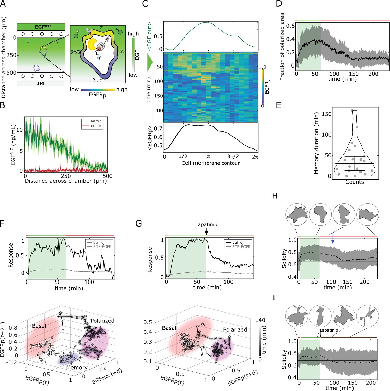
Molecular memory in polarized ${E G F R}^{m C i t r i n e}$ phosphorylation resulting from dynamical state-space trapping is translated to memory in polarized cell shape.

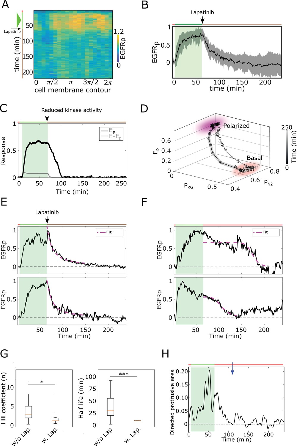
(A) Scheme of microfluidic EGF⁶⁴⁷-gradient experiment; Zoom: single-cell measurables. Cell membrane contour $[0, 2 π]$ (20 segments). $P T B$ - phosphotyrosine binding domain, $F P$ /star symbol - fluorescent protein, $E G F R_{p}$ - phosphorylated ${E G F R}^{m C i t r i n e}$ . Remaining symbols as in Figure 1B. (B) Quantification of EGF⁶⁴⁷ gradient profile (at $60 m i n$ , green) and after gradient wash-out (at $65 m i n$ , red). Mean ± s.d., N=4. (C) Exemplary quantification of, Top: Spatial projection of EGF⁶⁴⁷ around the cell perimeter. Gaussian fit of the spatial projection is shown. Middle: single-cell $E G F R_{p}$ kymograph. Data was acquired at 1 min intervals in live ${M C F 7 - E G F R}^{m C i t r i n e}$ cells subjected for $60 m i n$ to an EGF⁶⁴⁷ gradient. Other examples in Figure 2—figure supplement 1D. Bottom: respective spatial projection of $E G F R_{p}$ . Gaussian fit of the spatial projection is shown. Mean ± s.d. from n=20 cells, N=7 experiments in Figure 2—figure supplement 1C. (D) Average fraction of polarized plasma membrane area (mean ± s.d.). Single cell profiles in Figure 2—figure supplement 1G. (E) Quantification of memory duration in single cells (median±C.I.). In (D) and (E), n=20, N=7. (F) Top: Exemplary temporal profiles of phosphorylated $E G F R^{m C i t r i n e}$ (black) and $E G F^{647} - E G F R^{m C i t r i n e}$ (gray) corresponding to (C). Bottom: Corresponding reconstructed state-space trajectory (Figure 2—video 1) with denoted trapping state-space areas (colored). Thick/thin line: signal presence/absence. d - embedding time delay. (G) Equivalent as in (F), only in live MCF7-EGFR $S N_{P B}$ cell subjected to 1 hr EGF⁶⁴⁷ gradient (green shading), and 3 hr after wash-out with 1 µM Lapatinib. Corresponding kymograph shown in Figure 2—figure supplement 2A. Mean ± s.d. temporal profile from n=9, N=2 in Figure 2—figure supplement 2B. Bottom: Corresponding reconstructed state-space trajectory with state-space trapping (colored) (Methods, Figure 2—video 2). (H) Averaged single-cell morphological changes (solidity, mean ± s.d. from n=20, N=7). Average identified memory duration (blue arrow): $40 m i n$ . Top insets: representative cell masks at distinct time points. (I) Average solidity in ${M C F 7 - E G F R}^{m C i t r i n e}$ cells subjected to experimental conditions as in (G). Mean ± s.d. from n=9, N=2. Top insets: representative cell masks at distinct time points. In (**F-I**) green shaded area: EGF⁶⁴⁷ gradient duration; green/red lines: stimulus presence/absence. Brown line: Lapatinib stimulation. See also Figure 2—figure supplements 1 and 2.

Figure 2—source data 1 Source data for Figure 2.: https://cdn.elifesciences.org/articles/76825/elife-76825-fig2-data1-v2.xlsx
Download elife-76825-fig2-data1-v2.xlsx

Figure 2—figure supplement 1

Download asset Open asset

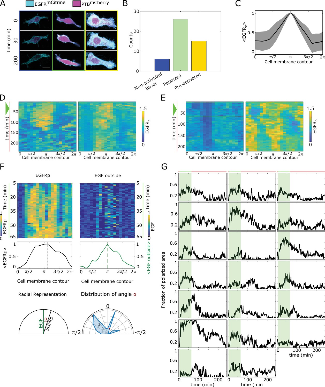
Quantification of ${E G F R}^{m C i t r i n e}$ phosphorylation polarization.

(A) Representative images / overlay of ${E G F R}^{m C i t r i n e}$ (cyan) and ${P T B}^{m C h e r r y}$ (magenta) prior to ( $0 m i n$ ), during ( $30 m i n$ ) and after ( $200 m i n$ ) ${M C F 7 - E G F R}^{m C i t r i n e}$ cells were subjected to $60 m i n$ EGF⁶⁴⁷ gradient. Columns: non-activated (blue), transiently polarized (green) and uniformly pre-activated (yellow). Scale bar: $15 μ m$ . (B) Distribution of single-cell responses corresponding to (A) from $N = 7$ experiments. (C) Average profile of the spatial projection of the fraction of phosphorylated ${E G F R}^{m C i t r i n e}$ from single-cell kymographs. For each cell, temporal average per spatial bin is calculated, and the final spatial profile was estimated as an average of a moving window of 7 points. Peaks of the single-cell distributions were shifted to $π$ before averaging. Mean ± s.d. from n=20 cells, N=7 experiments is shown. (D) Additional exemplary single-cell kymographs depicting polarized ${E G F R}^{m C i t r i n e}$ phosphorylation. Data acquisition and quantification as in Figure 2C. Triangle: gradient duration. (E) Same as in (D), only for non-activated (basal, left) and uniformly pre-acivated (right) ${E G F R}^{m C i t r i n e}$ phosphorylation. Triangle: gradient duration. (F) Quantification of direction of polarization of ${E G F R}^{m C i t r i n e}$ phosphorylation. Top: exemplary kymographs of $E G F R_{p}$ (left) and EGF⁶⁴⁷ outside the cells (right) during the gradient stimulation (60 min). Data corresponds to Figure 2C. Middle: respective spatial projection of $E G F R_{p}$ and EGF⁶⁴⁷. Average using a moving window of 7 bins is shown. Bottom: Schematic representation of identifying direction of polarization. Left: angle ( $α$ ) between $E G F R_{p}$ and EGF⁶⁴⁷ is estimated as the angle between the maxima of the spatial projections (shown in middle plots). Right: distribution of $α$ calculate from n=20 cells, N=7 experiments. (G) Temporal profiles of the estimated fraction of polarized area for single cells. Green shaded area: EGF⁶⁴⁷ gradient duration. The mean ± s.d. shown in Figure 2D.

Figure 2—figure supplement 1—source data 1 Source data for Figure 2—figure supplement 1.: https://cdn.elifesciences.org/articles/76825/elife-76825-fig2-figsupp1-data1-v2.xlsx
Download elife-76825-fig2-figsupp1-data1-v2.xlsx

Figure 2—figure supplement 2

Download asset Open asset

Memory in polarized $E G F R_{p}$ results from a dynamical ‘ghost’.

(A) Exemplary single-cell kymograph depicting phosphorylated ${E G F R}^{m C i t r i n e}$ for data acquired at 1 min intervals in live ${M C F 7 - E G F R}^{m C i t r i n e}$ cell subjected for 1 hr to EGF⁶⁴⁷ gradient, and 3 hr during gradient wash-out with 1 µM Lapatinib. (B) Average temporal profiles of plasma membrane ${E G F R}^{m C i t r i n e}$ phosphorylation of live ${M C F 7 - E G F R}^{m C i t r i n e}$ cells subjected for 1 hr to EGF⁶⁴⁷ gradient, and 3 hr during gradient wash-out with 1 µM Lapatinib. Related to Figure 2G. Mean ± s.d. from n=9, N=2 is shown. Green shaded area: EGF⁶⁴⁷ gradient. (C) In silico temporal profiles of $E_{p}$ (black) and $E - E_{p}$ (gray), when the kinase activity of the receptor is inhibited after gradient removal by decreasing the autocatalytic rate constant ( $α_{2} = 0.25$ ). Green shaded area: EGF gradient presence. (D) State-space trajectory corresponding to the example in (C), with denoted trapping state-space areas (colored). Thick/thin line: signal presence/absence. See also Figure 2—video 3. (E) Exemplary profiles of $E G F R_{p}$ (black) and corresponding fit with an inverse sigmoid function after gradient removal (magenta) of ${M C F 7 - E G F R}^{m C i t i r i n e}$ cell subjected for 1 hr to an EGF⁶⁴⁷ gradient, and 3 hr wash-out with 1 µM Lapatinib. (F), Same as in (E), but for cells without Lapatinib treatment. (G) Left: Hill coefficient estimated from single-cell fits with inverse sigmoid function as in (E, F). Right: Corresponding half-life estimates. n=23, N=5, (without Lapatinib) and n=12, N=5 (with Lapatinib). Error bars: median±95%C.I (H) Exemplary quantification of morphological changes using directed cell protrusion area for the cell shown in Figure 2C. Estimated memory duration: 43 min (blue arrow).

Figure 2—figure supplement 2—source data 1 Source data for Figure 2—figure supplement 2.: https://cdn.elifesciences.org/articles/76825/elife-76825-fig2-figsupp2-data1-v2.xlsx
Download elife-76825-fig2-figsupp2-data1-v2.xlsx

Figure 2—video 1

Download asset

Figure 2—video 2

Download asset

Figure 2—video 3

Download asset

Figure 3 with 5 supplements

Download asset Open asset

Cells display memory in directional migration toward recently encountered signals.

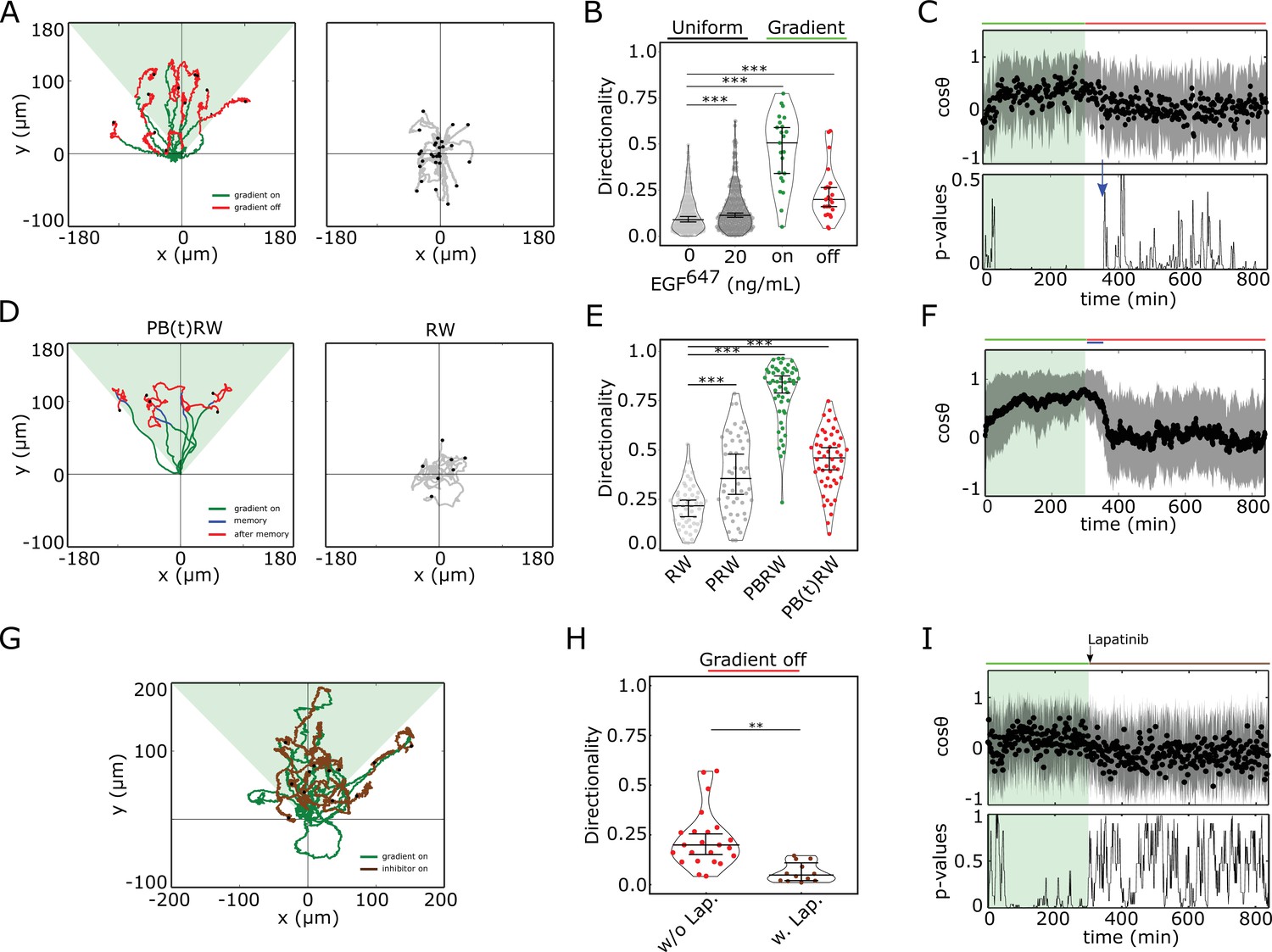
(A) Left: representative MCF10A single-cell trajectories. Green - 5 hr during and red line - 9 hr after dynamic EGF⁶⁴⁷ gradient (shaded). Exemplary cell in Figure 3—video 1. Right: Same as in (A), only 14 hr in continuous EGF⁶⁴⁷ absence. Black dots: end of tracks. (B) Directionality (displacement/distance) in MCF10A single-cell migration during 14 hr absence (0 ng/ml; n=245, N=3) or uniform 20 ng/ml EGF⁶⁴⁷ stimulation (n=297, N=3); 5 hr dynamic EGF⁶⁴⁷ gradient (green) and 9 hr during wash-out (red; n=23, N=5). p-values: ***p≤ 0.001, two-sided Welch’s t-test. Error bars: median±95%C.I. (C) Top: Projection of the cells’ relative displacement angles (mean ± s.d.; n=23, N=5) during (green shaded) and after 5 hr dynamic EGF⁶⁴⁷ gradient. Green/red lines: stimulus presence/absence. Bottom: Kolmogorov-Smirnov (KS) test p-values depicting end of memory in directional migration (blue arrow, $t = 350 m i n$ ). KS-test estimated using 5 time points window. For (**A-C**), data sets in Figure 3—figure supplements 1D and 2A. (D) Representative in silico single-cell trajectories. Left: PB(t)RW: Persistent biased random walk, bias is a function of time (green/blue trajectory part - bias on). Right: RW: random walk. (E) Corresponding directionality estimates from n=50 realizations, data in Figure 3—figure supplement 2D. PRW: persistent random walk. p-values: ***p≤ 0.001, two-sided Welch’s t-test. Error bars: median±95%C.I. (F) Same as in (C), top, only from the synthetic PB(t)RW trajectories. (G) MCF10A single-cell trajectories quantified 5 hr during (green) and 9 hr after (brown) dynamic EGF⁶⁴⁷ gradient (shading) wash-out with 3 µM Lapatinib. n=12, N=5. See also Figure 3—video 2. (H) Directionality in single-cell MCF10A migration after gradient wash-out with (brown, n=12, N=5) and without Lapatinib (red, n=23, N=5). p-values: **p≤ 0.01, KS-test. Error bars: median±95%C.I. (I) Same as in (C), only for the cells in (G). See also Figure 3—figure supplement 2H.

Figure 3—source data 1 Source data for Figure 3.: https://cdn.elifesciences.org/articles/76825/elife-76825-fig3-data1-v2.xlsx
Download elife-76825-fig3-data1-v2.xlsx

Figure 3—figure supplement 1

Download asset Open asset

Characterization of ${M C F 7 - E G F R}^{m C i t r i n e}$ and MCF10A single-cell migration.

(A) Identification of optimal EGF⁶⁴⁷ dose range for single-cell gradient migration assay for ${M C F 7 - E G F R}^{m C i t r i n e}$ (top) and MCF10A (bottom). Percentage of cells having motility greater than a displacement threshold ((Number of cell tracks with track length greater than threshold/Total number of cells)*100) is shown. (B) Top: Quantification of 5 hr dynamic EGF⁶⁴⁷ gradient at distinct time-points. Bottom: Corresponding quantification of the temporal evolution of the gradient slope. Percentage of gradient steepness: $((E G F_{(0)}^{647} - E G F_{(L)}^{647}) / E G F_{(0)}^{647}) * 100$ where $L$ is the length across the chamber. Mean ± s.d. from N=4 is shown. (C) Divergence plots depicting MCF7-EGFR^mCitrine single-cell trajectories quantified, left: 5 hr during (green) and for 9 hr after (red) dynamic EGF⁶⁴⁷ gradient duration (n=26, N=7); middle: 14 hr of 0 ng/ml EGF⁶⁴⁷ (subset of n=207 from n=426 is shown, N=2); and right: 14 hr of uniform 20 ng/ml EGF⁶⁴⁷ stimulation (subset of n=200 from n=456 is shown, N=2). (D) Same as in (C), only for MCF10A cells. Left: n=23, N=5; middle: n=245, N=3; right: n=297, N=3. Related to Figure 3A–C. Black dots: end of tracks.

Figure 3—figure supplement 1—source data 1 Source data for Figure 3—figure supplement 1.: https://cdn.elifesciences.org/articles/76825/elife-76825-fig3-figsupp1-data1-v2.xlsx
Download elife-76825-fig3-figsupp1-data1-v2.xlsx

Figure 3—figure supplement 2

Download asset Open asset

Characterization of single cell migration patterns.

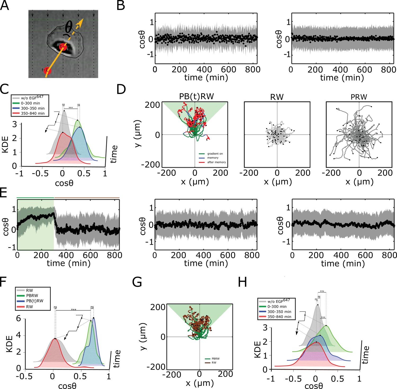
(A) Scheme of single-cell relative displacement angle estimation ( $\cos θ$ ). (B) Average $\cos θ$ from single MCF10A cell trajectories (mean ± s.d.), estimated over a 2 min interval upon, left: 0 ng/ml EGF⁶⁴⁷ (n=245, N=3); right: 20 ng/ml uniform EGF⁶⁴⁷ stimulation (n=297, N=3). Related to Figure 3A–C. (C) Kernel density estimates (KDE) of the distributions in (B) and Figure 3C top, in continuous EGF⁶⁴⁷ absence (gray), during 5 hr dynamic EGF⁶⁴⁷ gradient (green), after gradient wash-out: $t \in [300 m i n, 350 m i n]$ (blue) and $t \in [350 m i n, 840 m i n]$ (red). p-values: ***p≤ 0.001, ns: not significant, KS-test. (D) Synthetic single-cell trajectories (Equation 7, Materials and methods). Left: Persistent biased random walk PB(t)RW; middle: random walk (RW); right: Persistent random walk (PRW). Parameters: for PB(t)RW, $τ = 38.143$ , $b (t) = 0.134$ , $D = 2.207$ for $t \in [0 m i n, 350 m i n]$ (green,blue), $τ = 11.105$ , $b (t) = 0$ , $D = 0.425$ for $t \in [350 m i n, 840 m i n]$ (red); for RW, $τ = 11.105$ , $b (t) = 0$ , $D = 0.425$ ; for PRW, $τ = 38.143$ and $D = 2.207$ . (E) Same as in (B), only from the synthetic trajectories. Left: PB(t)RW with $τ = 38.143$ , $D = 2.207$ , $b (t) = 0.134$ for $t \in [0 m i n, 300 m i n]$ (green shading), $τ = 11.105$ , $D = 0.425$ , $b (t) = 0$ for $t \in [300 m i n, 840 m i n]$ , middle: RW; right: PRW. (F) Same as in (C), only from the synthetic trajectories. p-values: ***p≤ 0.001, ns: not significant, KS-test. (G) Synthetic single cell trajectories generated when PBRW is considered only in the time frame during gradient duration to mimic the experimental data in Figure 3G. Parameters as in (E, left). (H) Same as in (C), only for MCF10A cells stimulated for 5 hr with EGF⁶⁴⁷ gradient and 9 hr after wash-out with 3µM Lapatinib. Related to Figure 3I. p-values: ***p≤ 0.001, ns: not significant, KS-test.

Figure 3—figure supplement 2—source data 1 Source data for Figure 3—figure supplement 2.: https://cdn.elifesciences.org/articles/76825/elife-76825-fig3-figsupp2-data1-v2.xlsx
Download elife-76825-fig3-figsupp2-data1-v2.xlsx

Figure 3—figure supplement 3

Download asset Open asset

Quantifying duration of memory in directional migration from single-cell $\cos θ$ profiles.

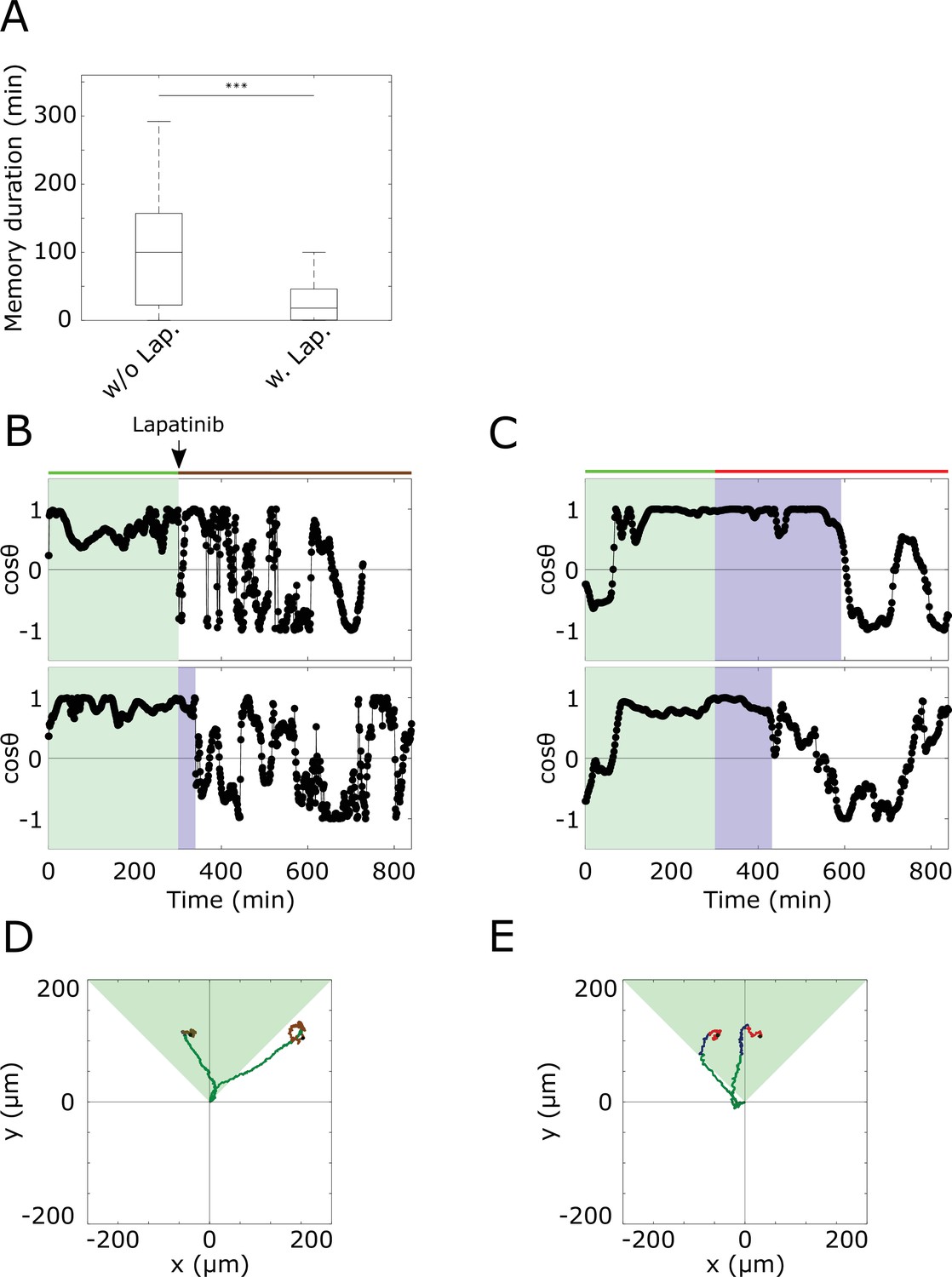
(A) Duration of memory in directional migration of MCF10A cells treated with a 5 hr dynamic EGF⁶⁴⁷ gradient (n=23, N=5; single cell tracks in Figure 3—figure supplement 1D), and MCF10A cells treated with a 5 hr dynamic EGF⁶⁴⁷ gradient, followed by 9 hr 3 µM Lapatinib during gradient wash-out (n=12, N=5, single cell tracks in Figure 3G). p-values: ***p≤0.001, two-sided Welch’s t-test. Error bars: median±95%C.I. Values estimated from single-cell $\cos θ$ plots. (B) Exemplary $\cos θ$ plots estimated from MCF10A cell motility trajectories. Cells were treated with a 5 hr dynamic EGF⁶⁴⁷ gradient, followed by 9 hr 3 µM Lapatinib during gradient wash-out. Green shaded area denotes EGF⁶⁴⁷ gradient interval, blue shaded area - time interval of identified memory in directional migration (Materials and methods). (C) Same as in (B), only without Lapatinib treatment. (D) Divergence plots of the cells shown in (B). Green part of the tracks denotes migration during gradient, blue - migration during identified memory phase after gradient removal, brown - random migration after gradient removal. Green shaded triangle: gradient direction. Black dots: end of tracks. (E) Divergence plots of the cells in (C). Color coding as in (D). Red: random migration after gradient wash-out.

Figure 3—figure supplement 3—source data 1 Source data for Figure 3—figure supplement 3.: https://cdn.elifesciences.org/articles/76825/elife-76825-fig3-figsupp3-data1-v2.xlsx
Download elife-76825-fig3-figsupp3-data1-v2.xlsx

Figure 3—video 1

Download asset

Figure 3—video 2

Download asset

Figure 4 with 8 supplements

Download asset Open asset

Working memory enables history-dependent single-cell migration in changing chemoattractant field.

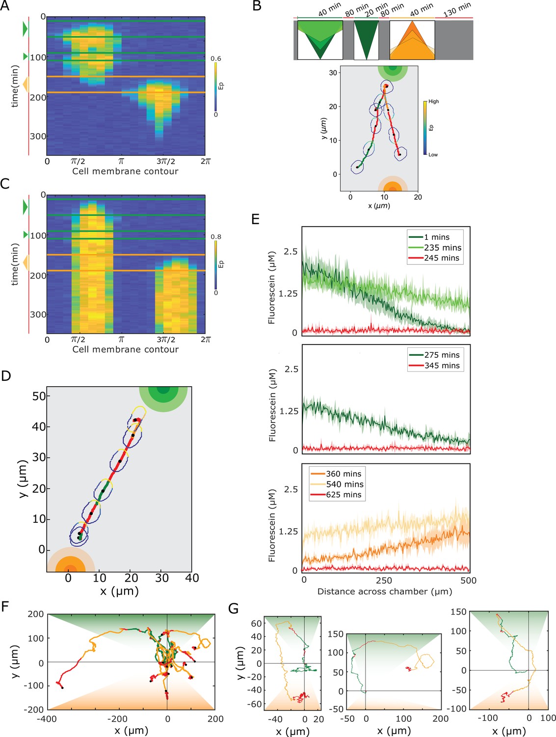
(A) Scheme of dynamic spatial-temporal growth factor field implemented in the simulations and experiments. Green(orange)/red: gradient presence/absence. (B) In silico cellular response to the sequence of gradients as depicted in (A), showing changes in EGFR activity, cellular morphology and respective motility trajectory over time. Trajectory color coding corresponding to that in (A), cell contour color coding with respective $E_{p}$ values as in Figure 1E. Cell size is magnified for better visibility. See also Figure 4—figure supplement 1A, Figure 4—video 1. (C) Representative MCF10A single-cell trajectory and cellular morphologies at distinct time-points, when subjected to dynamic EGF⁶⁴⁷ gradient field as in (A) (gradient quantification in Figure 4—figure supplement 1E). Trajectory color coding corresponding to that in (A). See also Figure 4—video 4. Full data set in Figure 4—figure supplement 1F. (D) Projection of cells’ relative displacement angles ( $\cos θ$ ) depicting their orientation towards the respective localized signals. Mean ± s.d. from n=12, N=5 is shown. (E) Corresponding kernel density estimates (intervals and color coding in legend). p-values: ***, p≤0.001, ns: not significant, KS-test.

Figure 4—source data 1 Source data for Figure 4.: https://cdn.elifesciences.org/articles/76825/elife-76825-fig4-data1-v2.xlsx
Download elife-76825-fig4-data1-v2.xlsx

Figure 4—figure supplement 1

Download asset Open asset

Single-cell navigation in changing growth factor fields.

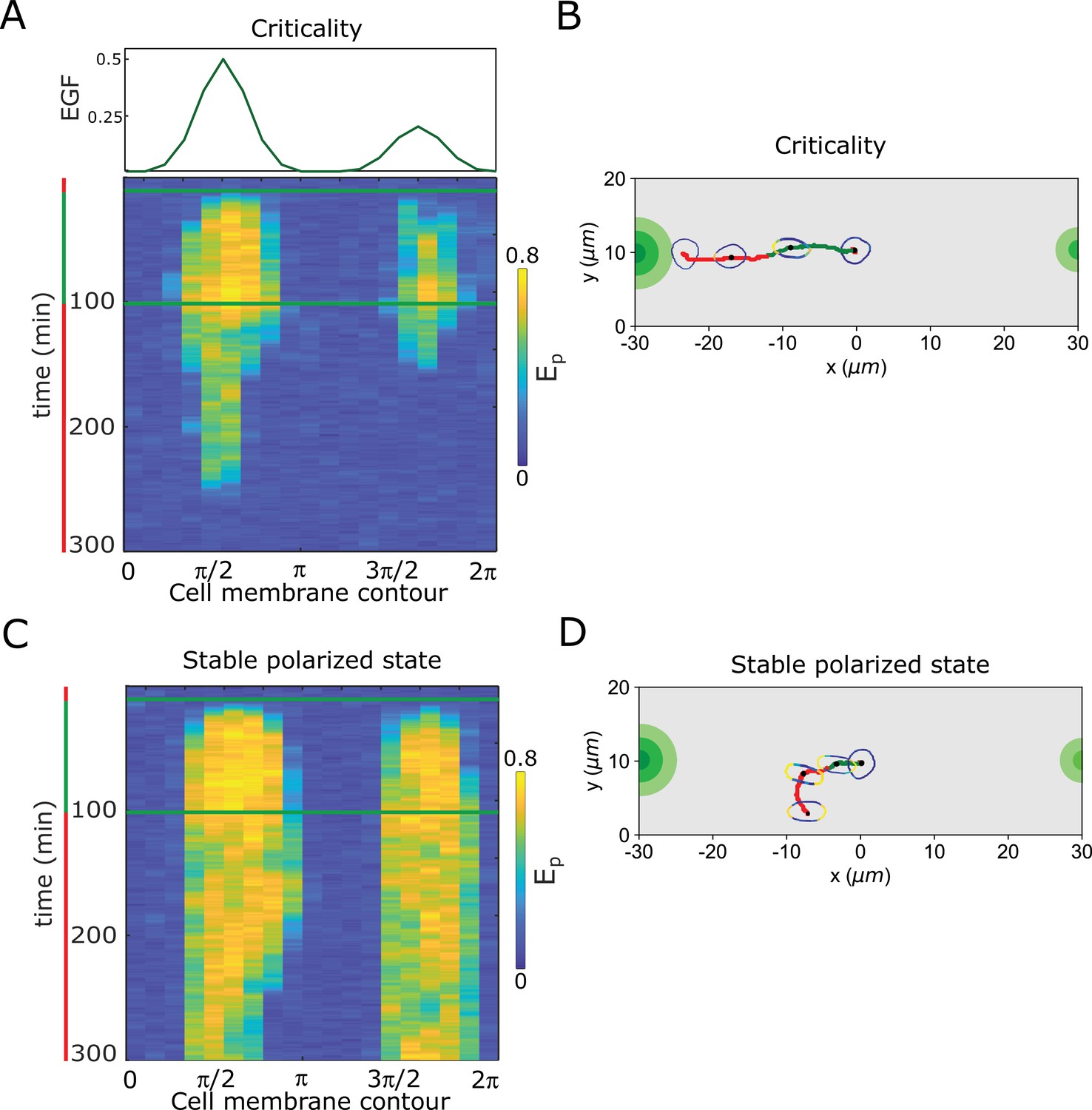
(A) In silico obtained $E_{p}$ kymograph corresponding to Figure 4B. Parameters in Materials and methods. (B) In silico cellular response to a sequence of gradients as depicted on top, showing changes in EGFR phosphorylation, cellular morphology and respective motility trajectory over time. Trajectory color coding corresponding to scheme on top, cell contour color coding with respective $E_{p}$ values as in Figure 1E. Cell size is magnified for better visibility. See also Figure 4—video 2. (C) $E_{p}$ kymograph obtained for organization in the stable polarized state, when a cell is subjected to the gradient filed in Figure 4A. (D) Corresponding changes in cellular morphology and respective motility trajectory over time. Trajectory and $E_{p}$ color coding as in (B). Cell size is magnified for better visibility. See also Figure 4—video 3. (E) Quantification of a 15 hr dynamic fluorescein gradient at distinct time-points. Mean ± s.d. from N=3 is shown. (F) Divergence plots depicting MCF10A single-cell trajectories quantified during migration in dynamic EGF⁶⁴⁷ gradient field shown in (E). n=12, N=5. Trajectory color-coding corresponding to the scheme in Figure 4A. (G) Zoomed exemplary single-cell trajectories from (F).

Figure 4—figure supplement 1—source data 1 Source data for Figure 4—figure supplement 1.: https://cdn.elifesciences.org/articles/76825/elife-76825-fig4-figsupp1-data1-v2.xlsx
Download elife-76825-fig4-figsupp1-data1-v2.xlsx

Figure 4—figure supplement 2

Download asset Open asset

Resolving simultaneous signals with opposed localisation is optimal at criticality.

(A) Top: Position of two simultaneous EGF gradients with different amplitudes in the numerical simulation. Bottom: Representative in silico kymograph of EGFR phosphorylation ( $E_{p}$ ) for organization of the system at criticality. (B) Corresponding changes in cellular morphology and motility trajectory over time. Trajectory and $E_{p}$ color coding as in (A). Cell size is magnified for better visibility. See also Figure 4—video 5. (C) Same as in (A), only for organization in the stable polarized state. (D) Same as in (B), only for organization in the stable polarized state (corresponding to C). See also Figure 4—video 6.

Figure 4—video 1

Download asset

Figure 4—video 2

Download asset

Figure 4—video 3

Download asset

Figure 4—video 4

Download asset

Figure 4—video 5

Download asset

Figure 4—video 6

Download asset

Author response image 1

Download asset Open asset

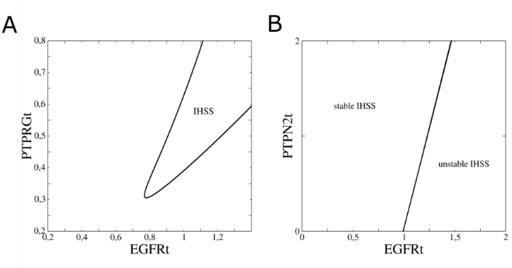
In-depth bifurcation analysis of the EGFR network.

(A) Two-parameter bifurcation analysis (EGFRt vs. PTPRGt) characterizing the range where pitchfork bifurcations (black line) emerge. (B) Same as in a, only when PTPN2t instead of PTPRGt is considered.

Author response image 2

Download asset Open asset

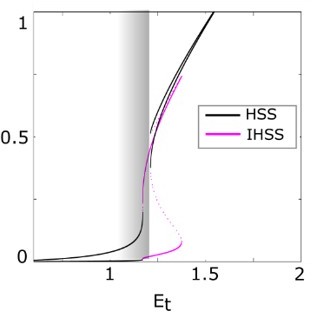
Generic principles of the symmetry breaking mechanism.

Unfolding of the pitchfork bifurcation – the bifurcation diagram of the full system as in a., only when a local EGF gradient signal is present.

Author response image 3

Download asset Open asset

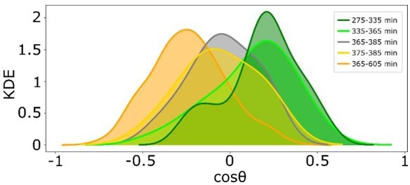
Quantification of the time intevbal in which cells revert their direction of migration, as extracted from KDE distributions of reversal of gradient migration data in Figure 4 —figure supplement 1F.

Author response image 4

Download asset Open asset

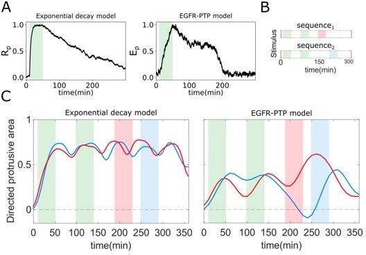
Optimal response to changing environments is rendered by metastable dynamics.

(A) Response to single gradient stimulation using an exponential decay model for receptor activity dynamics (Equation 1) with slow dephosphorylation kinetics (left); and using the EGFR-PTP model with metastable “ghost” state. (B) Two distinct sequences of spatial-temporal gradient fields. (C) Directed protrusive area estimated from in-silico cell shape changes during stimulus sequence 1 (red) and sequence 2 (blue) for the exponential decay model (left) and EGFR-PTP model (right). Parameters for the exponential decay model: α = 1.5, R_t = 1, β = 0.5 × 10⁻².

Author response image 5

Download asset Open asset

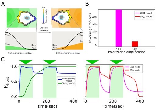
Comparison of information processing features between existing polarisation models (LEGI, Turing, Wavepinning) and the proposed SN_PB mechanism.

(A) Schematic of gradient reversal. (B) Quantification of the time for polarization reversal and corresponding polarization amplification $(\frac{R_{rev}}{R_{front}})$ at stimulus ratio, $(\frac{S_{rev}}{S_{front}}) = 2$ . (C) Time series of signaling response at the leading edge (R_front1) of the cell upon two consecutive gradients from the same direction for Wave-pinning and Turing models (left), and LEGI and SN_PB model (right).

Tables

Key resources table

Reagent type (species) or resource	Designation	Source or reference	Identifiers	Additional information
Cell line (Homo sapiens)	MCF-7	ECACC	Cat.No.86012803
Cell line (Homo sapiens)	MCF10A	ATCC	CRL-10317
Recombinant DNA reagent	EGFR-mCitrine	Baumdick et al., 2015
Recombinant DNA reagent	PTB-mCherry	Fueller et al., 2015
Recombinant DNA reagent	cCbl-BFP	Fueller et al., 2015
Peptide, recombinant protein	Fibronectin	Sigma-Aldrich	F0895-1MG
Peptide, recombinant protein	Collagen	Sigma-Aldrich	C9791-50MG
Chemical compound, drug	Lapatinib	Cayman chemicals	Cay11493-10
Chemical compound, drug	Hoechst 33,342	Thermo Fisher Sc.	62,249
Chemical compound, drug	Dulbecco’s modified Eagle’s medium (DMEM)	PAN Biotech	Cat. # P04-01500
Chemical compound, drug	MEM Amino Acids Solution (50 x)	PAN Biotech	Cat. # P08 32,100
Chemical compound, drug	Penicillin- Streptomycin	PAN Biotech	Cat. # P06 07100
Chemical compound, drug	Fetal Bovine Serum	Sigma-Aldrich	Cat. # F7524
Chemical compound, drug	EGF	Sigma-Aldrich	Cat. # E9644
Chemical compound, drug	Hydrocortisone	Sigma-Aldrich	Cat. #H-0888
Chemical compound, drug	Cholera toxin	Sigma-Aldrich	Cat. #C-8052
Chemical compound, drug	Insulin	Sigma-Aldrich	Cat. #I-1882
Chemical compound, drug	Horse Serum	Invitrogen	26050088
Chemical compound, drug	FuGENE6	Promega	E2691
Software, algorithm	Python	Python software foundation	RRID:SCR_008394
Software, algorithm	Matlab	MathWorks	RRID:SCR_001622
Software, algorithm	XPPAUT	http://www.math.pitt.edu/~bard/xpp/xpp.html
Software, algorithm	Trackmate	https://doi.org/10.1016/j.ymeth.2016.09.016
Software, algorithm	Fiji, ImageJ	https://doi.org/10.1038/nmeth.2019
Other	EGF-Alexa647	Sonntag et al., 2014	Prof. Luc Brunsveld, University of Technology, Eindhoven	Methods
Other	Cellasic ONIX plates	Merck Chemicals	M04G-02-5PK	Methods

Additional files

Supplementary file 1 Model parameters. Details included also in Methods.: https://cdn.elifesciences.org/articles/76825/elife-76825-supp1-v2.xlsx
Download elife-76825-supp1-v2.xlsx
Transparent reporting form: https://cdn.elifesciences.org/articles/76825/elife-76825-transrepform1-v2.pdf
Download elife-76825-transrepform1-v2.pdf

Download links

A two-part list of links to download the article, or parts of the article, in various formats.

Downloads (link to download the article as PDF)

Open citations (links to open the citations from this article in various online reference manager services)

Mendeley

Cite this article (links to download the citations from this article in formats compatible with various reference manager tools)

Akhilesh Nandan
Abhishek Das
Robert Lott
Aneta Koseska

(2022)

Cells use molecular working memory to navigate in changing chemoattractant fields

eLife 11:e76825.

https://doi.org/10.7554/eLife.76825

Share this article

Cite this article

In silico manifestation of metastable polarized membrane signaling, as a mechanism for sensing changing spatial-temporal signals.

Features of receptor activity for different organization in parameter space.

Corresponding to Figure 1F.

Molecular memory in polarized EGFRmCitrine phosphorylation resulting from dynamical state-space trapping is translated to memory in polarized cell shape.

Figure 2—source data 1

Quantification of EGFRmCitrine phosphorylation polarization.

Figure 2—figure supplement 1—source data 1

Memory in polarized E⁢G⁢F⁢Rp results from a dynamical ‘ghost’.

Figure 2—figure supplement 2—source data 1

Corresponding to Figure 2F.

Corresponding to Figure 2G.

Corresponding to Figure 2—figure supplement 2D.

Cells display memory in directional migration toward recently encountered signals.

Figure 3—source data 1

Characterization of MCF7−EGFRmCitrine and MCF10A single-cell migration.

Figure 3—figure supplement 1—source data 1

Characterization of single cell migration patterns.

Figure 3—figure supplement 2—source data 1

Quantifying duration of memory in directional migration from single-cell cos⁡θ profiles.

Figure 3—figure supplement 3—source data 1

Corresponding to Figure 3A.

Corresponding to Figure 3G.

Working memory enables history-dependent single-cell migration in changing chemoattractant field.

Figure 4—source data 1

Single-cell navigation in changing growth factor fields.

Figure 4—figure supplement 1—source data 1

Resolving simultaneous signals with opposed localisation is optimal at criticality.

Corresponding to Figure 4B.

Corresponding to Figure 4—figure supplement 1B.

Corresponding to Figure 4—figure supplement 1C, D.

Corresponding to Figure 4C.

Corresponding to Figure 4—figure supplement 2A, B.

Corresponding to Figure 4—figure supplement 2C, D.

In-depth bifurcation analysis of the EGFR network.

Generic principles of the symmetry breaking mechanism.

Quantification of the time intevbal in which cells revert their direction of migration, as extracted from KDE distributions of reversal of gradient migration data in Figure 4 —figure supplement 1F.

Optimal response to changing environments is rendered by metastable dynamics.

Comparison of information processing features between existing polarisation models (LEGI, Turing, Wavepinning) and the proposed SNPB mechanism.

Supplementary file 1

Transparent reporting form

Downloads (link to download the article as PDF)

Open citations (links to open the citations from this article in various online reference manager services)

Cite this article (links to download the citations from this article in formats compatible with various reference manager tools)

Molecular memory in polarized ${E G F R}^{m C i t r i n e}$ phosphorylation resulting from dynamical state-space trapping is translated to memory in polarized cell shape.

Quantification of ${E G F R}^{m C i t r i n e}$ phosphorylation polarization.

Memory in polarized $E G F R_{p}$ results from a dynamical ‘ghost’.

Characterization of ${M C F 7 - E G F R}^{m C i t r i n e}$ and MCF10A single-cell migration.

Quantifying duration of memory in directional migration from single-cell $\cos θ$ profiles.

Comparison of information processing features between existing polarisation models (LEGI, Turing, Wavepinning) and the proposed SN_PB mechanism.