Balance between breadth and depth in human many-alternative decisions
- Center for Brain and Cognition, and Department of Information and Communication Technologies, Universitat Pompeu Fabra, Spain
- Department of Experimental and Health Sciences, Universitat Pompeu Fabra, Spain
- Insitució Catalana de la Recerca i Estudis Avançats (ICREA), Spain
- Serra Húnter Fellow Programme, Universitat Pompeu Fabra, Spain
Figures
Figure 1
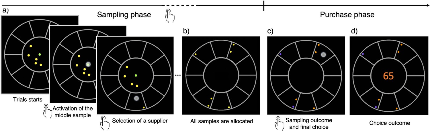
The breadth-depth (BD) apricot task.
Human participants allocate a finite search capacity (coins) to learn about the quality of good apricots in different suppliers (sampling phase) and then make a final purchase of 100 apricots from one of the sampled suppliers (purchase phase). Each black section of the wheel represents a different supplier. The number of coins represents the search capacity of the participants on each trial and varies randomly from trial to trial within a finite range (see Materials and methods). The available coins (panel a; yellow green dots) at any time during the trial are displayed within the centre of the wheel. To allocate the coins to suppliers, participants have first to click on the designated active coin displayed at the centre (green dot) and then select the supplier to sample from (panel a) – both touch screen events are indicated by a large grey dot. One of the inactive (yellow) coins is then automatically activated and displayed, in green, at the centre. This sequence repeats until all coins are allocated. Then, each of the allocated samples turn either orange, representing a good-quality apricot, or purple, representing a bad-quality apricot (panel c). Finally, after this information is revealed, the participant selects one of the sampled suppliers for the final purchase of 100 apricots (with a touch screen, indicated by a large grey dot) and the choice outcome is immediately displayed (panel d).
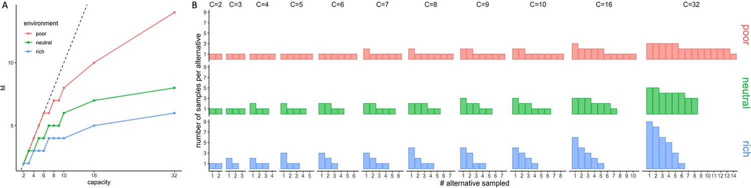
Figure 2
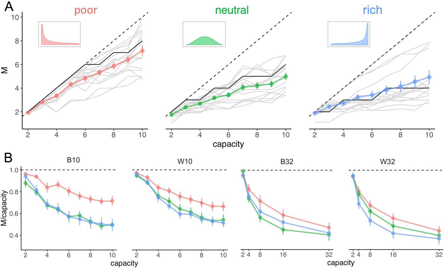
Number of sampled suppliers increases with capacity and is strongly sensitive to the richness of the environment, consistent with theoretical predictions.
(A) Number of alternatives sampled as a function of capacity averaged across participants (points), for each of the three different environments (colours), for the low-capacity between-subject design (B10). Dashed lines indicate unit slope line. Optimal observer predictions are displayed in black and grey lines represent individual data. Error bars correspond to s.e.m. (B) Number of alternatives sampled divided by capacity as a function of capacity. Colour code as in panel A. Samples sizes per environment condition: designs B10 and B32: n=15, designs W10 and W32: n=18.
Figure 3
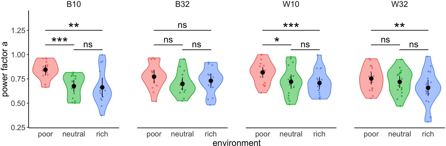
Participants’ strategy is modulated by the richness of the environment.
Distribution of power factors extracted from fitting a linear model to values vs. capacity in a log-log scale. Colour dots represent subjects, black dots represent means across participants, and bars are 95% confidence intervals. Results of post hoc comparisons are displayed according to adjusted p-values (‘ns’: p>0.05, ‘**’: p<0.01, ‘***’: p<0.001). Samples sizes per environment condition: designs B10 and B32: n=15, designs W10 and W32: n=18.
Figure 4 with 1 supplement
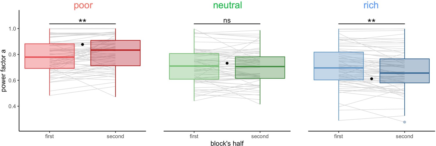
Participants’ sampling strategy gets closer to the optimal breadth-depth (BD) trade-offs with experience.
Distribution of the power factor in the power-law model when fitting the number of alternatives sampled M as a function of the capacity in each environment, separately for each block’s half (median split on the number of trials). Each line connects a subject, black dots represent the power factor when fitting the optimal BD trade-offs. Results of post hoc comparisons are displayed according to adjusted p-values (‘ns’: >0.1, ‘**’: <0.01). Lower and upper hinges correspond to the 1st and 3rd quartiles and vertical lines represent the interquartile range (IQR) multipled by 1.5. Sample sizes n=66.
Figure 4—figure supplement 1
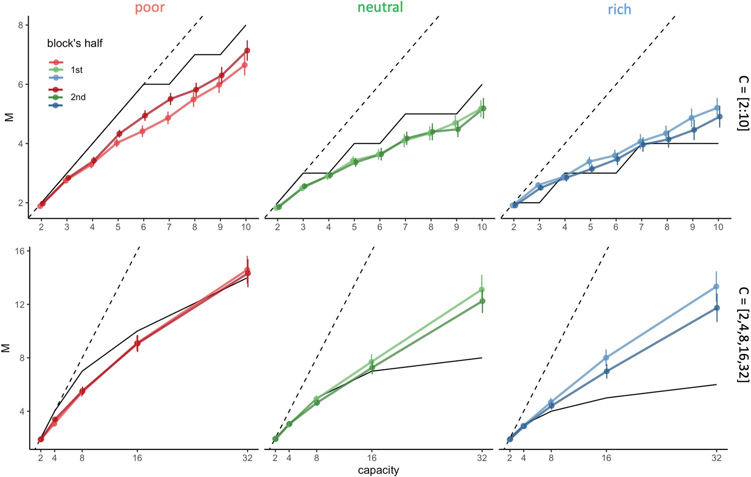
Participants’ sampling strategy gets closer to the optimal breadth-depth (BD) trade-offs as time passes within a block.
(A) Number of alternatives sampled M as a function of the capacity depending on the environment richness, the capacity range (small: top, large: bottom) and the block’s half (median split on the number of trials). Dashed lines indicate unit slope line and black lines the optimal BD trade-offs. Bars represent s.e.m. Sample sizes per environment and capacity range condition: n=33.
Figure 5 with 2 supplements
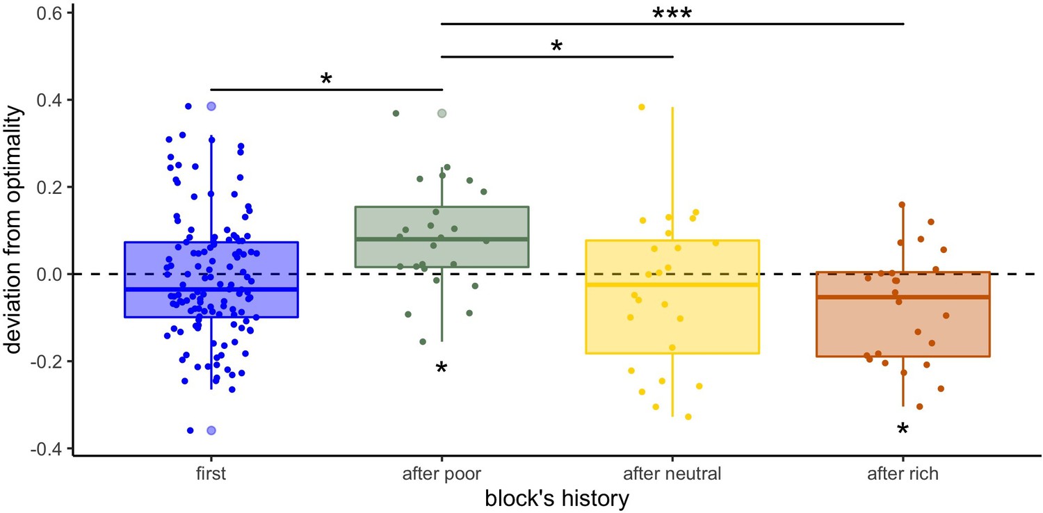
Participants’ sampling strategy is affected by the previous environment presented.
Distribution of the individual deviation from optimality (difference between power factors fitting the data and the optimal BD trade-off) for each block’s history (presented first or independently, or after another environment). ’*’: p<0.05, ‘**’: p<0.01, ‘***’: p<0.001. Lower and upper hinges correspond to the 1st and 3rd quartiles and vertical lines represent IQR*1.5. Sample sizes: 'first': n=126, 'after poor/neutral/rich': n=24.
Figure 5—figure supplement 1
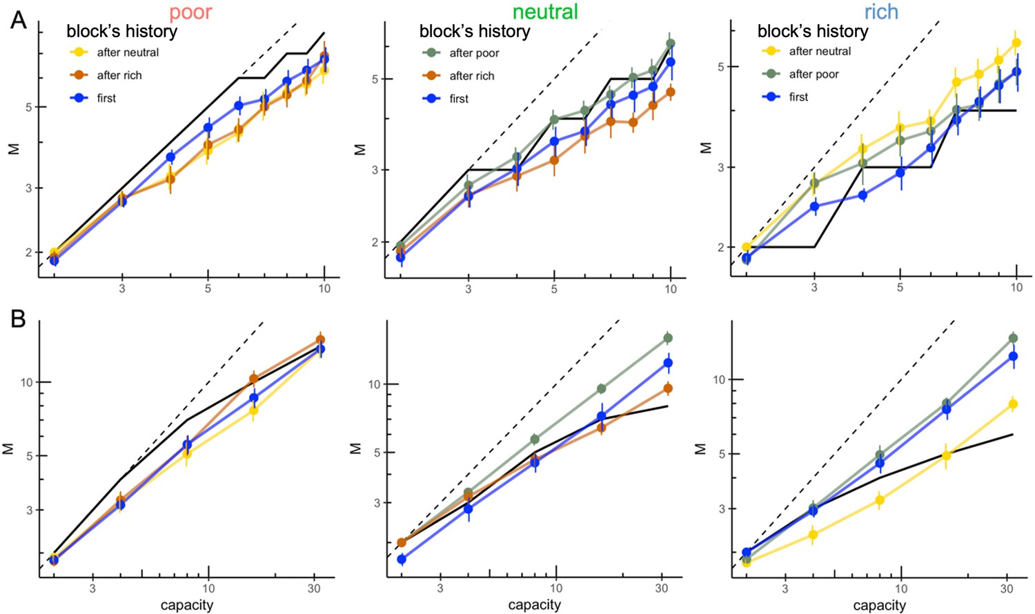
Participants’ sampling strategy seems to be influenced by the previous environment presented.
Number of alternatives sampled as a function of capacity averaged across participants (points) for the three different environments (left: poor, centre: neutral, right: rich) and depending on its presentation order (colours; first environment presented or presented after a poor, neutral, or rich environment), for within-subject design with narrow (W10, panel A) or wide capacities (W32, panel B). Sample sizes in each environment condition: 'first': n=6, 'after poor/neutral/rich': n=12.
Figure 5—figure supplement 2
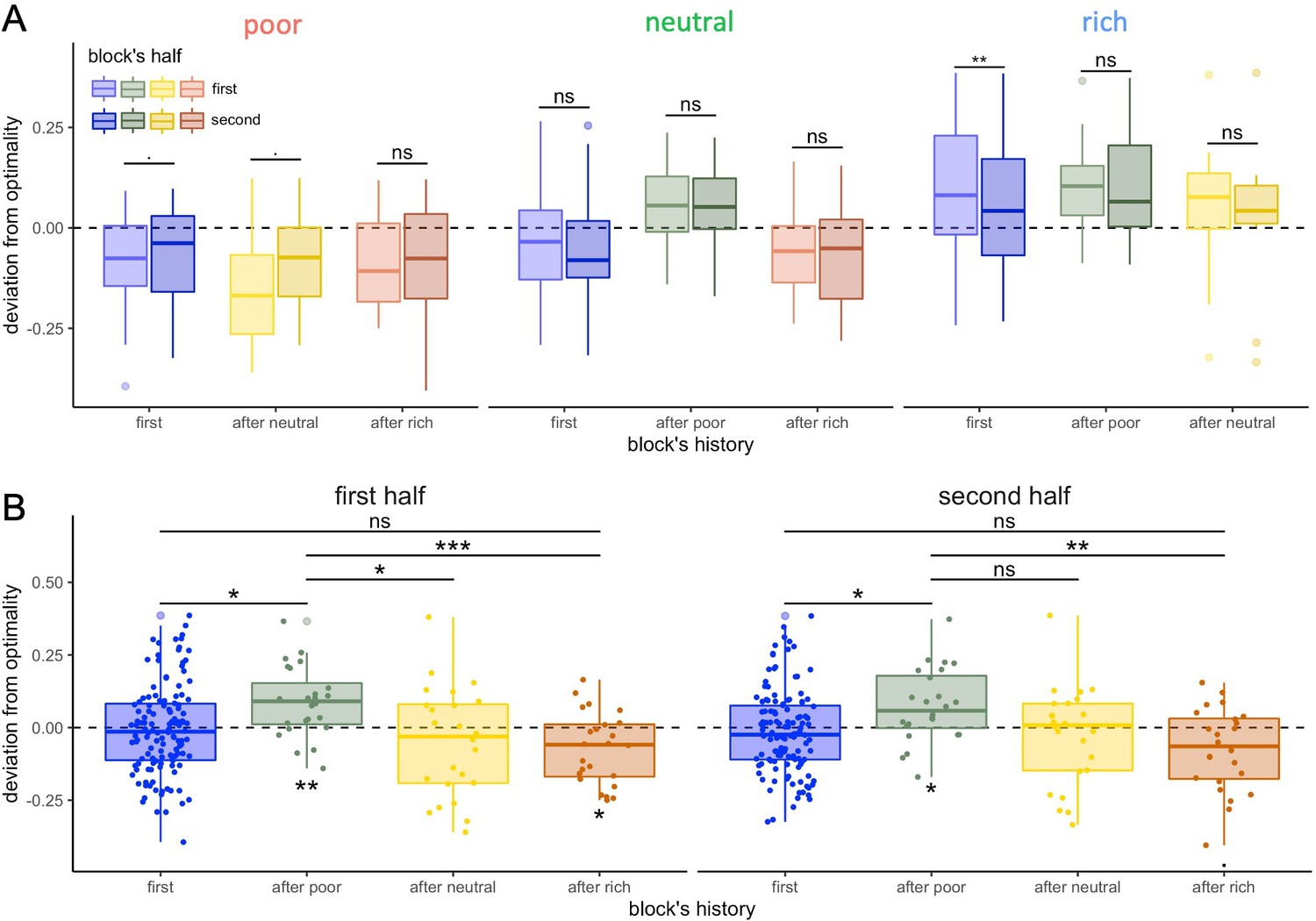
Participants tend to be closer to optimal in the second compared to first part of the block but contamination effects due to the environment change do not fully dissipate.
(A) Distribution of the individual deviation from optimality (difference between power factors fitting the data and the optimal BD trade-off) depending on the block’s history: presented first (or alone) or after another environment for each environment condition individually (A) and for each block’s half individually (B). ‘ns’: p>0.1, ‘.’: p<0.1,’*’: p<0.05, ‘**’: p<0.01, ‘***’: p<0.001. Lower and upper hinges correspond to the 1st and 3rd quartiles and vertical lines represent IQR*1.5. Sample sizes (A): 'first': n=42, 'after poor/neutral/rich': n=24 in each condition, (B): 'first': n=126, 'after poor/neutral/rich': n=24 in each condition.
Figure 6 with 1 supplement
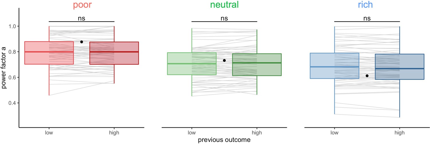
Participants’ sampling strategy is not affected by the outcome obtained in the previous trial.
Distribution of the power factor in the power-law model when fitting the number of alternatives sampled M as a function of the capacity in each environment, depending on the magnitude of the reward obtained in the previous trial (median split on the trial reward inside capacity and environment conditions). Each line connects a subject, black dots represent the power factor when fitting the optimal breadth-depth (BD) trade-offs. Results of post hoc comparisons are displayed according to adjusted p-values (‘ns’: >0.1). Lower and upper hinges correspond to the 1st and 3rd quartiles and vertical lines represent IQR*1.5. Sample sizes per environment condition: n=66.
Figure 6—figure supplement 1
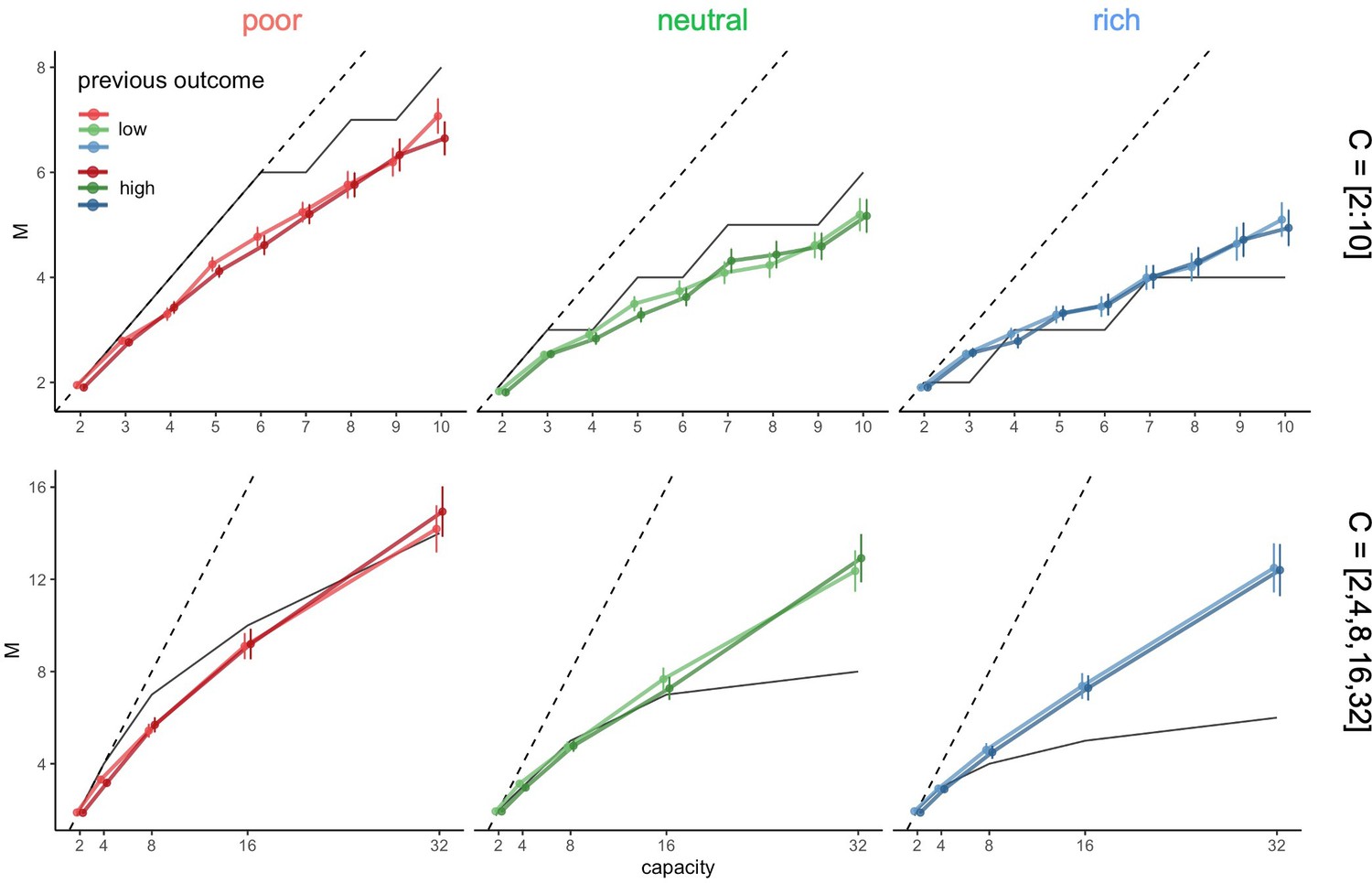
Participants’ sampling strategy is not affected by the outcome obtained in the previous trial.
(A) Number of alternatives sampled M as a function of the capacity depending on the environment richness, the capacity range (small: top, large: bottom) and the magnitude of the amount of reward accumulated (median split). Dashed lines indicate unit slope line and black lines are the optimal breadth-depth (BD) trade-offs. Bars represent s.e.m. Sample sizes per environment and capacity range condition: n=33.
Figure 7 with 1 supplement

Participants resample more often and with more samples the previously chosen alternative when it was associated with high reward but it has no impact on the breadth-depth (BD) trade-off adaptation to the environment richness.
Fraction of trials for which the previously selected alternative (at trial t) was sampled on the consecutive trial (at trial t+1) (resampling fraction) (A) and fraction of the capacity allocated in this alternative (B), depending on its previous associated outcome (at trial t, median split: low and high) overall. Grey lines connect individual data. ‘***’: p<0.001. Lower and upper hinges correspond to the 1st and 3rd quartiles and vertical lines represent IQR*1.5. Sample size: n=126. (C) Averaged power factors extracted from fitting a linear model to values M vs. capacity in a log-log scale for participants showing a preference to resample previously rewarding alternatives (≥5%, ‘biased’) or not (‘unbiased’). Errors bars represent s.e.m. Sample size for each experiment paradigm for the biased (B10: 23, W10: 10, B32: 15, W32: 12) and unbiased participants (B10: 22, W10: 8, B32: 30, W32: 6).
Figure 7—figure supplement 1
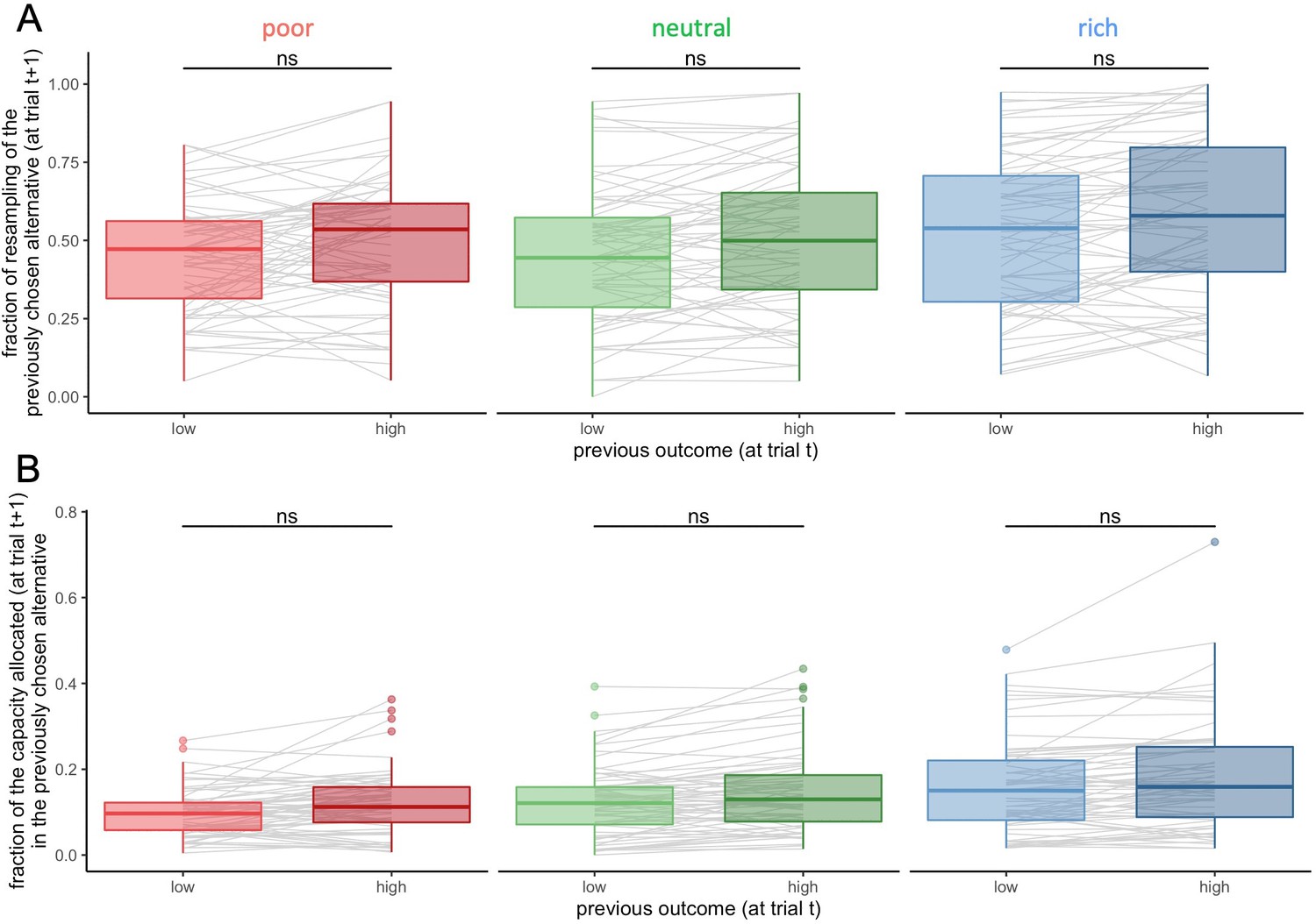
Participants’ resampling bias for highly rewarded alternatives is not found at the environment level.
Fraction of trials for which the previously selected alternative (at trial t) was sampled on the consecutive trial (at trial t+1) (resampling fraction) (A) and fraction of the capacity allocated in this alternative (B), depending on its previous associated outcome (at trial t, median split: low and high) inside each environment. Grey lines connect individual data. ‘ns’: p>0.1. Lower and upper hinges correspond to the 1st and 3rd quartiles and vertical lines represent IQR*1.5. Sample sizes per environment condition: n=66.
Figure 8 with 4 supplements

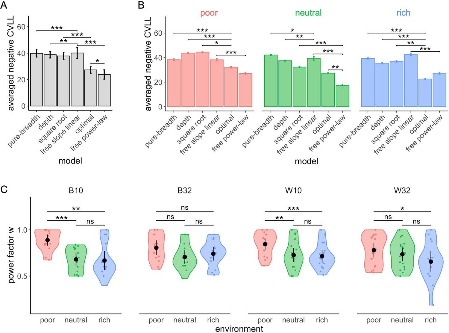
The free power-law model is better at predicted participants’ sampling strategy than both the optimal and other heuristic models (using binomial distributed noise).
Averaged negative cross-validated log-likelihood (CVLL) across participants for each model overall (A) and in each environment (B). Results of pair-wise comparisons are displayed according to adjusted p-values (‘*’: p<0.05, ‘**’: p<0.01, ‘***’: p<0.001) and error bars correspond to s.e.m. Sample sizes (A): n=126, (B): n=66 for each environment condition. (C) Distribution of the power factor in the free power model. Each colour dot represents a subject, black dots represent distribution means, and bars 95% confidence intervals. Results of post hoc comparisons are displayed according to adjusted p-values (‘ns’: p>0.05, ‘**’: p<0.01, ‘***’: p<0.001). Samples sizes per environment condition: designs B10 and B32: n=15, designs W10 and W32: n=18.
Figure 8—figure supplement 1
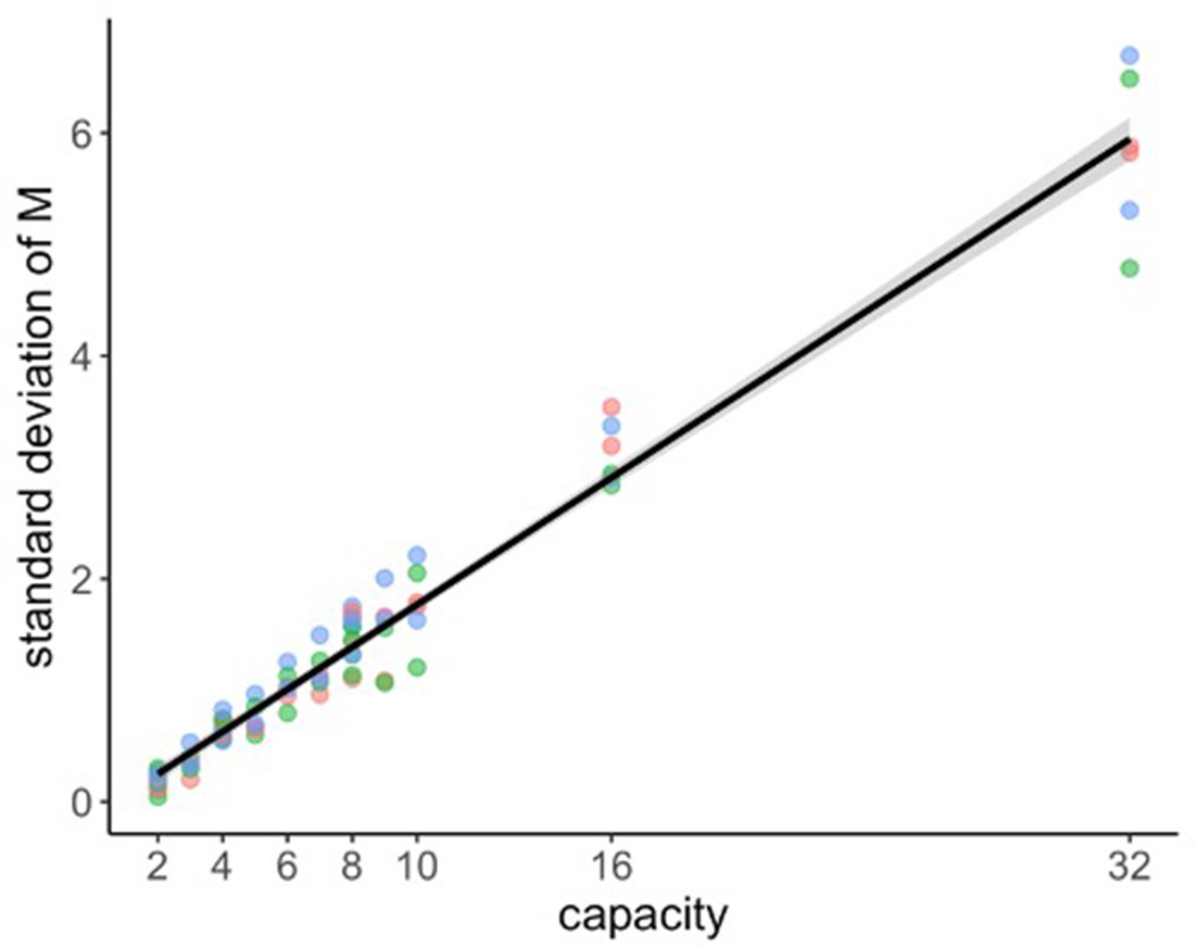
The standard deviation of the number of alternatives sampled increases linearly with the capacity.
Each point represents the standard deviation of averaged across participants for each experimental design, environment, and capacity. Sample size n=126.
Figure 8—figure supplement 2
The free power-law model is better at predicting participants’ sampling strategy than both the optimal and other heuristics models using Gaussian distributed noise.
Averaged negative cross-validated log-likelihood (CVLL) across participants for each model overall (A) and in each environment (B). Results of pair-wise comparisons are displayed according to adjusted p-values (‘*’: p<0.05, ‘**’: p<0.01, ‘***’: p<0.001) and error bars correspond to s.e.m. (C) Distribution of the power factor w in the free power model. Each colour dot represents a subject, black dots represent distribution means, and bars 95% confidence intervals. Results of post hoc comparisons are displayed according to adjusted p-values (‘ns’: p>0.05, ‘**’: p<0.01, ‘***’: p<0.001). Samples sizes per environment condition: designs B10 and B32: n=15, designs W10 and W32: n=18.
Figure 8—figure supplement 3
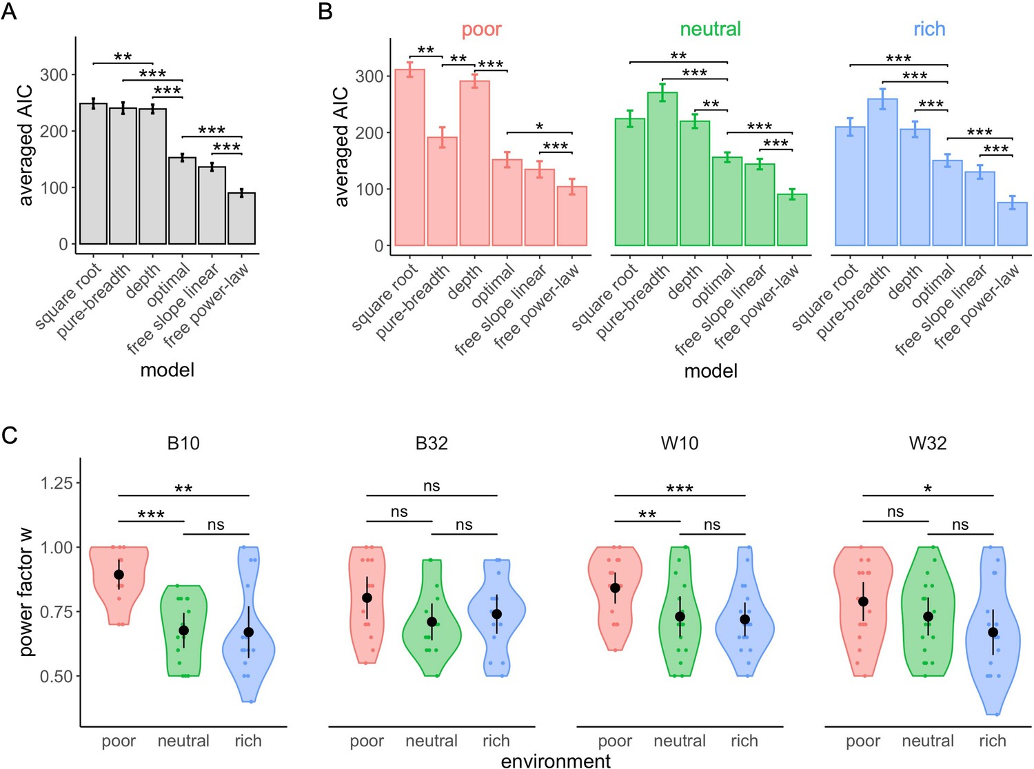
The free power-law model is better at predicting participants’ sampling strategy than both the optimal and other heuristics models using binomial distributed noise.
Averaged negative Akaike information criteria (AIC) across participants for each model overall (A) and in each environment (B). Results of pair-wise comparisons are displayed according to adjusted p-values (‘*’: p<0.05, ‘**’: p<0.01, ‘***’: p<0.001) and error bars correspond to s.e.m. (C) Distribution of the power factor in the free power model. Each colour dot represents a subject, black dots represent distribution means, and bars 95% confidence intervals. Results of post hoc comparisons are displayed according to adjusted p-values (‘ns’: p>0.05, ‘**’: p<0.01, ‘***’: p<0.001). Samples sizes per environment condition: designs B10 and B32: n=15, designs W10 and W32: n=18.
Figure 8—figure supplement 4
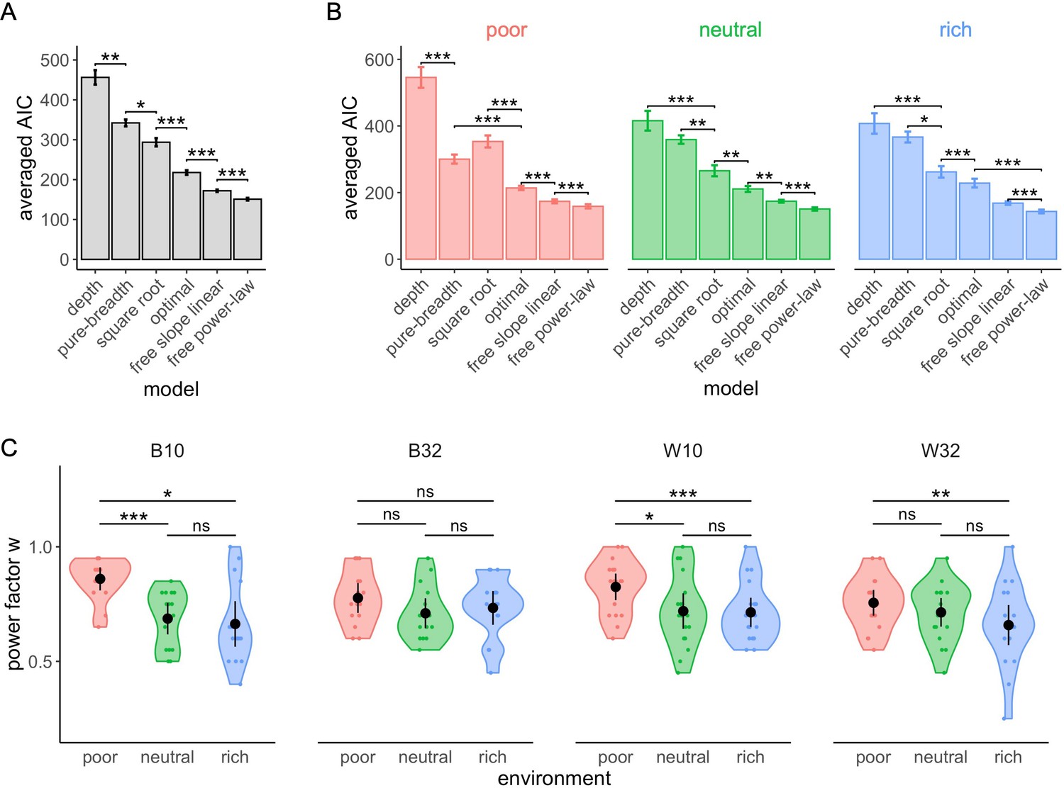
The free power-law model is better at predicting participants’ sampling strategy than both the optimal and other heuristics models using Gaussian distributed noise.
Averaged negative Akaike information criteria (AIC) across participants for each model overall (A) and in each environment (B). Results of pair-wise comparisons are displayed according to adjusted p-values (‘*’: p<0.05, ‘**’: p<0.01, ‘***’: p<0.001) and error bars correspond to s.e.m. (C) Distribution of the power factor in the free power model. Each colour dot represents a subject, black dots represent distribution means, and bars 95% confidence intervals. Results of post hoc comparisons are displayed according to adjusted p-values (‘ns’: p>0.05, ‘**’: p<0.01, ‘***’: p<0.001). Samples sizes per environment condition: designs B10 and B32: n=15, designs W10 and W32: n=18.
Figure 9
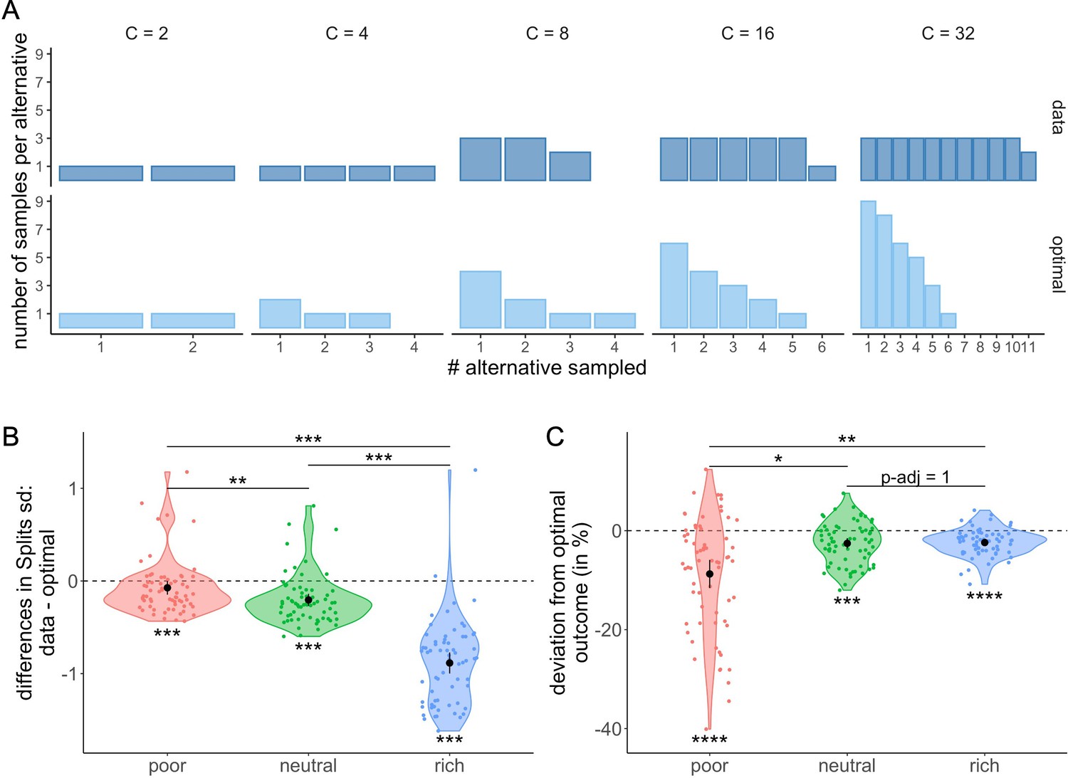
Participants tend to allocate homogeneously the samples across the selected alternatives, which largely differs from the optimal allocation, and impacts the outcome.
(A) Number of samples allocated to each sampled alternative depending on the sampling capacity . Upper panels: most frequent allocation of samples observed across participants in the rich environment (design B32) as a function of capacity. Lower panels: allocation of samples maximizing the reward (optimal). (B) Distributions of the differences between observed and optimal standard deviations of the distribution of samples among the selected alternatives in each environment (e.g. if and 2 samples are allocated in a first alternative while the last 2 samples are each allocated in a second and third alternative, the standard deviation of this sample allocation would correspond to ). Note that more homogeneous distributions tend to lead to lower standard deviations. (C) Distributions of the differences between observed and optimal outcomes in each environment. In the last two panels, dots represent participants and include all trials for which the optimal number of alternatives sampled was inferior to capacity ( – see Materials and methods for more details). Below each distribution are presented results of one-sample Wilcoxon tests (‘**’: <0.01, ‘***’: <0.001) and above are presented results of Wilcoxon tests between each environment (‘ns’: >0.05, ‘*’: <0.05,‘**’: <0.01,‘***’: <0.001). All p-values have been adjusted with Bonferroni corrections. Sample sizes for each environment condition: n=66.
Figure 10

Participants prefer the depth- over the breadth-focused strategy.
The fraction of trials for which alternatives are sampled according to the depth- (dark-orange) vs. breadth-focused (light-orange) strategy is shown for each number of sampled alternatives () and capacity (). Example of a sampling sequence of alternatives {a,b,c,d} with and for in breadth-focused strategy: {a,a,b,c,c,d,d} and breadth-focused strategy: {a,b,c,d,d,a,c}. This analysis includes all trials for which >1 (no pure-depth) and <C (no pure-breadth). Only combinations of with at least 10 trials (over all participants) were displayed.
Appendix 1—figure 1
Optimal strategies as a function of both capacity and environment richness.
(A) Optimal number of alternatives sampled as a function of the capacity for each of the three environments (colours). Dashed line indicates unit slope line (pure breadth). (B) Optimal number of samples allocated to each sampled alternative depending on the sampling capacity and the environment richness.
Appendix 2—figure 1

Participants’ sampling strategy deviates from optimality and tends to be tilted toward depth at low capacity and breadth at high capacity.
Difference between the optimal () and the observed () number of alternatives sampled averaged across all participants for each capacity and environment (coloured lines). Error bars represent the standard error of the mean and significant deviations from 0 (dashed line) are marked as follows: ‘*’: , ‘**’: , ‘***’: , ‘****’: .
Appendix 3—figure 1

Participants present a motor bias when sampling.
(A–B) Fraction of samples allocated in each alternative, in the designs with 10 alternatives (W10 and B10, A) and 32 alternatives (W32 and B32, B). Bars represent s.e.m.
Appendix 4—figure 1
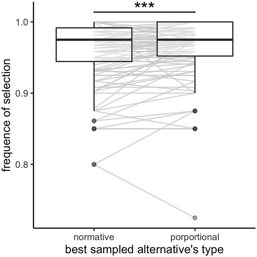
Participants select more often the best sampled alternative independently, compared to dependently, on the priors of the environment.
Frequency of selection of the best sampled alternative calculated based on the normative outcome (depends on the environment richness) and the proportional outcome. Grey lines connect individual data. Lower and upper hinges correspond to the 1st and 3rd quartiles and vertical black lines represent IQR*1.5. `***`: p<0.001. Sample sizes per condition: n=126.
Videos
Video 1
Demonstration video of the task (design W10).
Tables
Table 1
Summary of the experimental designs.
| Design | Capacity | N suppliers | N trials | N subject | |
|---|---|---|---|---|---|
| W10 | Within-subject | 2–10 | 10 | 216 | 18 |
| B10 | Between-subject | 2–10 | 10 | 72 | 45 |
| W32 | Within-subject | 2,4,8,16,32 | 32 | 120 | 18 |
| B32 | Between-subject | 2,4,8,16,32 | 32 | 40 | 45 |
Table 2
Participants’ sampling strategy significantly deviates from optimality.
Values of the factor predicted (first row) or observed (averaged across participants ± s.d., second row) depending on capacity using a power-law function with free exponent and fixed intercept (see Materials and methods for more details). Results of comparisons between factors using one-sample t-tests with Bonferroni corrections (third row) show that participants’ sampling strategy extracted from fitting the number of alternatives sampled is significantly tilted towards depth in the poor and neutral (tendency) environments compared to optimality, while in the rich environment participants are sampling in a breather way than predicted.
| Environment Value of power factor | Poor | Neutral | Rich |
|---|---|---|---|
| Optimal (predicted) | 0.877 | 0.732 | 0.612 |
| Data (observed) | 0.795±0.118 | 0.705±0.127 | 0.688±0.152 |
| Comparison |
Table 3
Summary of the pair-wise comparisons (Wilcoxon matched pairs signed-ranks test) of the fourfolds averaged cross-validated log-likelihoods (CVLL) between all six models using binomial distributed noise.
p-Values are adjusted with Bonferroni corrections and significative differences (p<0.05) are highlighted in bold. Models are ordered from worst (depth) to best (free power law).
| Pure breadth | Square root | Optimal | Linear | Power | |
|---|---|---|---|---|---|
| Depth | |||||
| Pure breadth | |||||
| Square root | |||||
| Optimal | |||||
| Linear |
Additional files
-
Transparent reporting form
- https://cdn.elifesciences.org/articles/76985/elife-76985-transrepform1-v2.pdf
-
Supplementary file 1
Participants’ sampling strategy deviates from optimality and tends to be tilted toward depth at low capacity and breadth at high capacity.
- https://cdn.elifesciences.org/articles/76985/elife-76985-supp1-v2.docx
-
Supplementary file 2
Post-hoc comparisons between deviations from optimality in power factors extracted from fitting the power law model to BD trade-offs in first and second halves of blocks separately.
- https://cdn.elifesciences.org/articles/76985/elife-76985-supp2-v2.docx
-
Supplementary file 3
Post-hoc analyses of the deviations from optimality in power factors extracted from fitting the power law model to BD trade-offs in first and second halves of blocks separately.
- https://cdn.elifesciences.org/articles/76985/elife-76985-supp3-v2.docx
-
Supplementary file 4
Post-hoc comparisons between deviations from optimality in power factors extracted from fitting the power law model to BD trade-offs in first and second halves of blocks separately.
- https://cdn.elifesciences.org/articles/76985/elife-76985-supp4-v2.docx
-
Supplementary file 5
Summary of the pair-wise comparisons of the 4-folds averaged CVLL between all six models using Gaussian distributed noise.
- https://cdn.elifesciences.org/articles/76985/elife-76985-supp5-v2.docx
-
Supplementary file 6
Summary of the comparisons between the averaged individual 4-fold CVLL in each environment and experimental design using Gaussian distributed noise.
- https://cdn.elifesciences.org/articles/76985/elife-76985-supp6-v2.docx
-
Supplementary file 7
Summary of the pair-wise comparisons of the individual AIC between all six models using Binomial distributed noise.
- https://cdn.elifesciences.org/articles/76985/elife-76985-supp7-v2.docx
-
Supplementary file 8
Summary of the comparisons between the individual AIC in each environment and experimental design using Binomial distributed noise.
- https://cdn.elifesciences.org/articles/76985/elife-76985-supp8-v2.docx
-
Supplementary file 9
Summary of the pair-wise comparisons of the individual AIC between all six models using Gaussian distributed noise.
- https://cdn.elifesciences.org/articles/76985/elife-76985-supp9-v2.docx
-
Supplementary file 10
Summary of the comparisons between the individual AIC in each environment and experimental design using Gaussian distributed noise.
- https://cdn.elifesciences.org/articles/76985/elife-76985-supp10-v2.docx
Download links
A two-part list of links to download the article, or parts of the article, in various formats.
Downloads (link to download the article as PDF)
Open citations (links to open the citations from this article in various online reference manager services)
Cite this article (links to download the citations from this article in formats compatible with various reference manager tools)
Balance between breadth and depth in human many-alternative decisions
eLife 11:e76985.
https://doi.org/10.7554/eLife.76985


