Uncertainty-based inference of a common cause for body ownership
- Department of Neuroscience, Karolinska Institutet, Sweden
- Center for Neural Science and Department of Psychology, New York University, United States
Figures
Figure 1
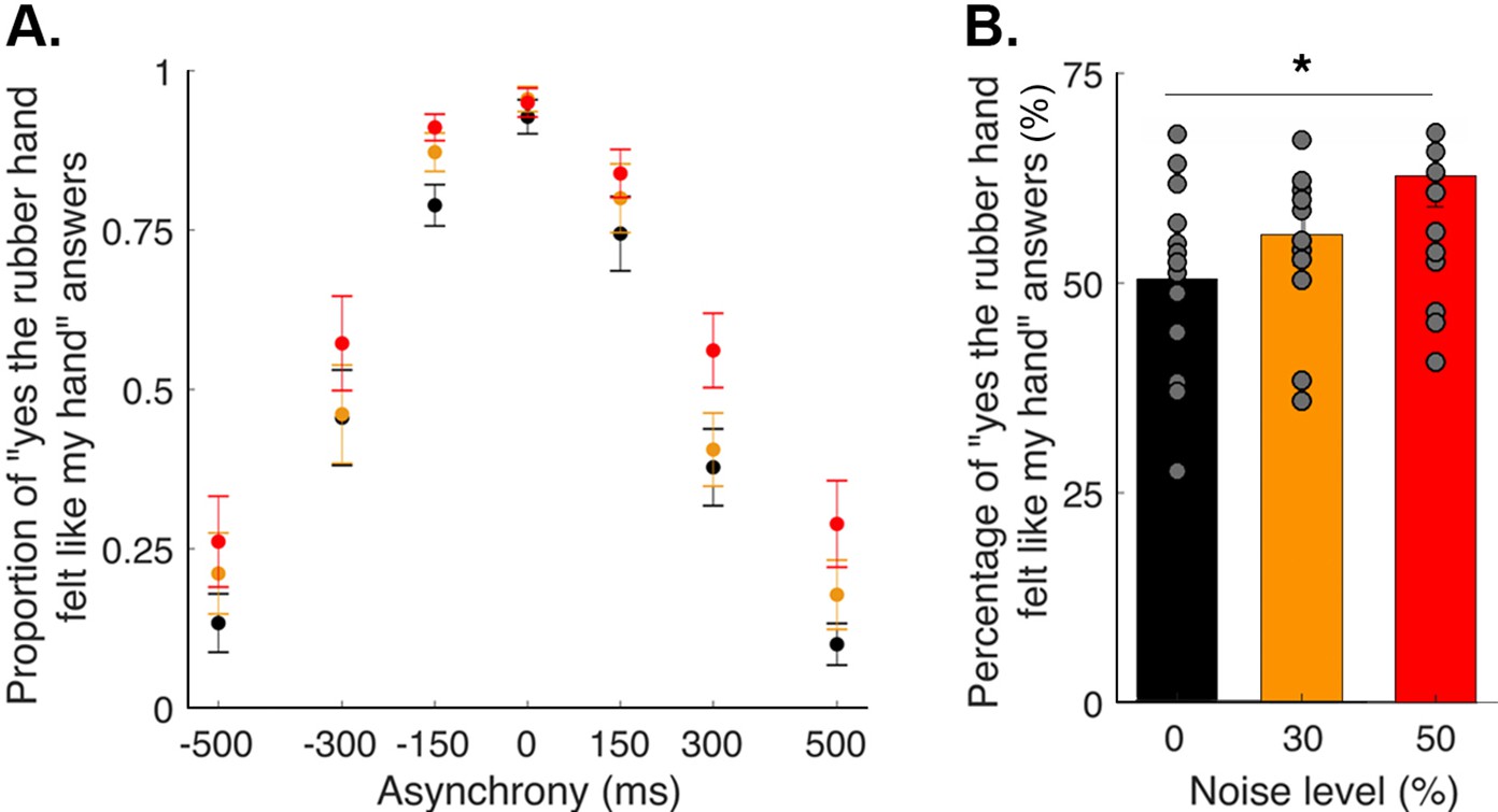
Elicited rubber hand illusion under different levels of visual noise.
(A) Colored dots represent the mean reported proportion of elicited rubber hand illusions (± SEM) for each asynchrony for the 0 (black), 30 (orange), and 50% (red) noise conditions. (B) Bars represent how many times in the 84 trials the participants answered ‘yes (the rubber hand felt like my own hand)’ under the 0 (black), 30 (orange), and 50% (red) noise conditions; gray dots are individual data points. There was a significant increase in the number of ‘yes’ answers when the visual noise increased * p<0.001.
-
Figure 1—source data 1
Sum of "yes" answer for the different asynchrony and noise levels tested in the body ownership judgment task used in Figure 1.
- https://cdn.elifesciences.org/articles/77221/elife-77221-fig1-data1-v3.xlsx
Figure 2 with 5 supplements
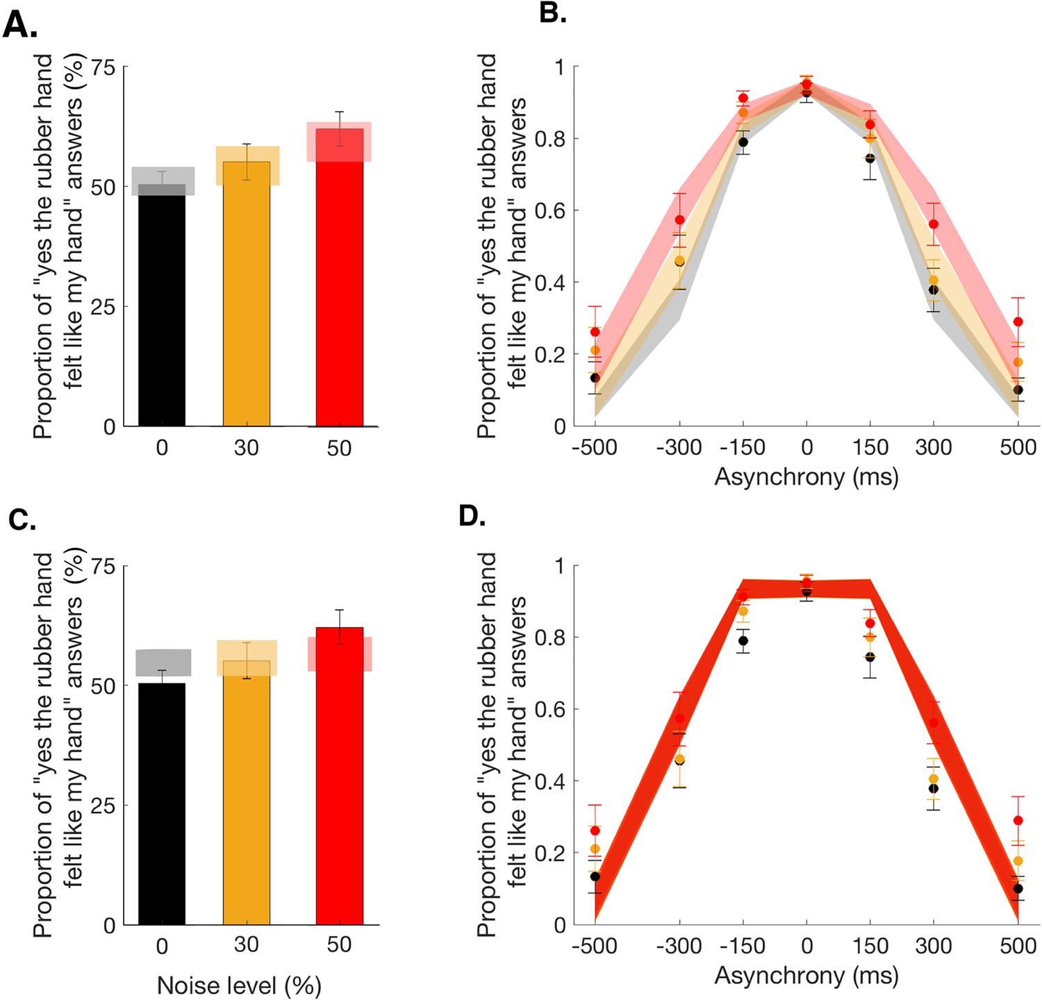
Observed and predicted detection responses for body ownership in the rubber hand illusion.
Bars represent how many times across the 84 trials participants answered ‘yes’ in the 0 (black), 30 (orange), and 50% (red) noise conditions (mean ± SEM). Lighter polygons denote the Bayesian causal inference (BCI) model predictions (A) and fixed-criterion (FC) model predictions (C) for the different noise conditions. Observed data refer to 0 (black dots), 30 (orange dots), and 50% (red dots) visual noise and corresponding predictions (mean ± SEM; gray, yellow, and red shaded areas, respectively) for the BCI model (B) and FC model (D).
-
Figure 2—source data 1
Parameter estimates for the BCI* model use in Figure 2.
- https://cdn.elifesciences.org/articles/77221/elife-77221-fig2-data1-v3.xlsx
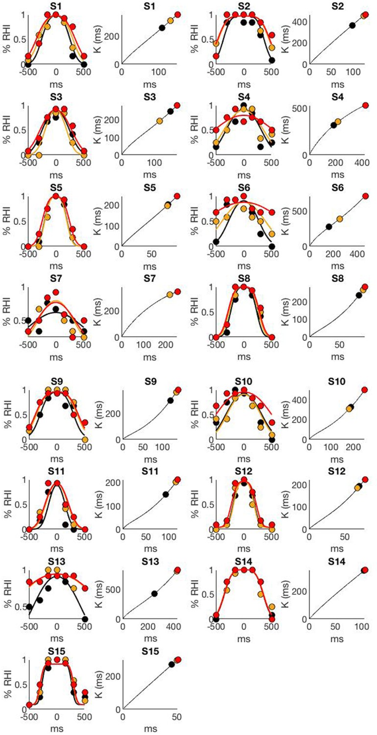
Figure 2—figure supplement 1
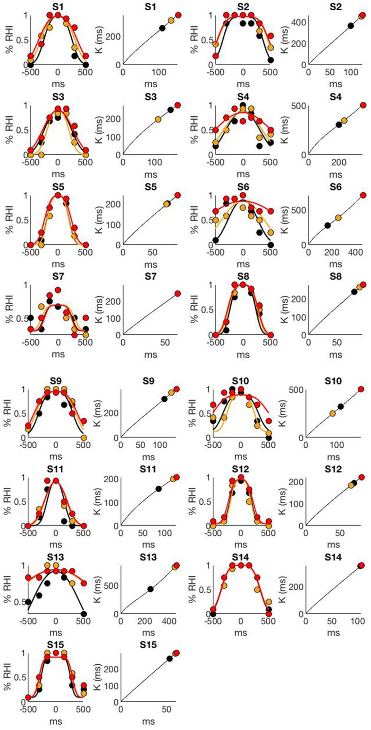
Individual data and BCI model fit.
The figure display two plots per participant, the "yes [the rubber hand felt like my own hand]" answers as a function of visuotactile asynchrony (dots) and corresponding BCI model fit (curves) are plotted on the left; the right plot represents the evolution of the BCI decision criteria with sensory noise and the 3 dots highlight the decision criteria for the conditions tested in the present study. As in the main text, black, orange, and red correspond to the 0%, 30%, and 50% noise levels, respectively.
Figure 2—figure supplement 2
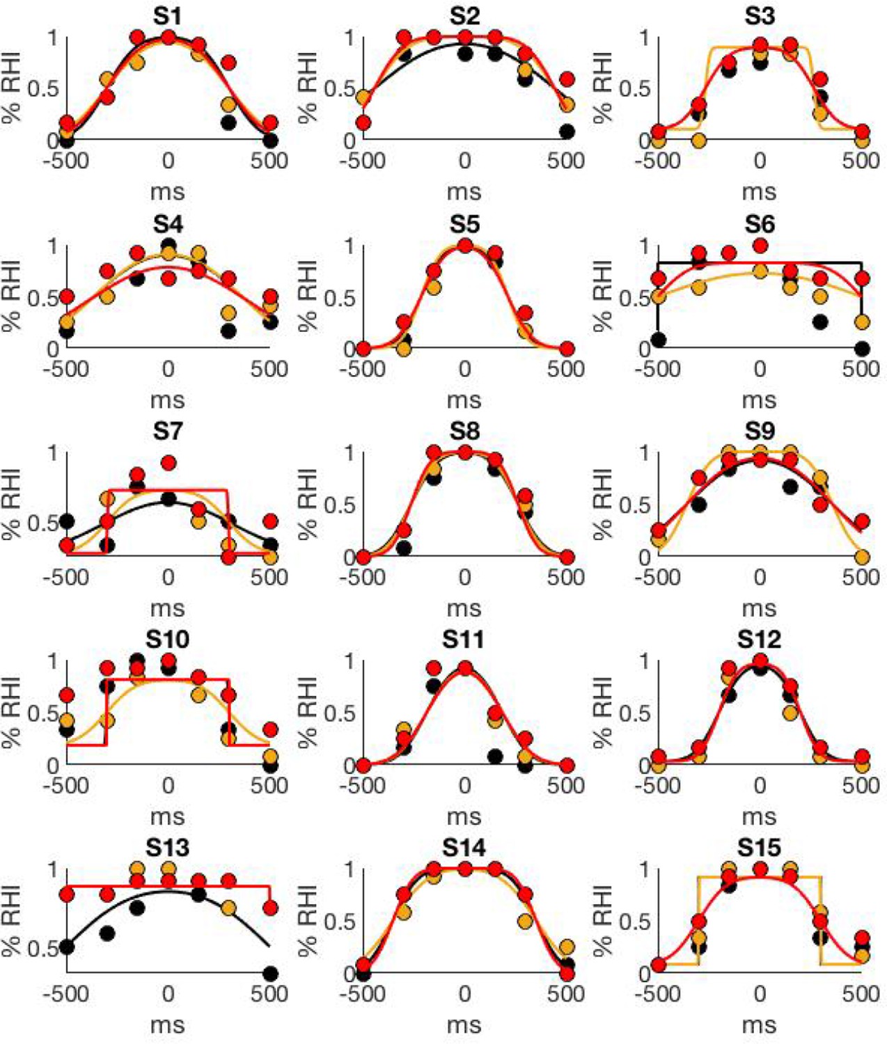
Individual data and FC model fit.
The figure display one plot per participant, the "yes [the rubber hand felt like my own hand]" answers as a function of visuo-tactile asynchrony (dots) and corresponding FC (non Baysesian) model t (curves) are plotted. As in the main figure, black, orange, and red correspond to the 0%, 30%, and 50% noise levels, respectively.
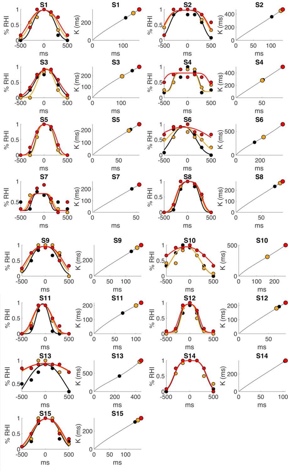
Figure 2—figure supplement 3
Individual data and BCI* model fit.
The figure display two plots per participant, the "yes [the rubber hand felt like my own hand]" answers as a function of visuo-tactile asynchrony (dots) and corresponding BCI* model fit (curves) are plotted on the left; the right plot represents the evolution of the BCI decision criteria with sensory noise and the 3 dots highlight the decision criteria for the conditions tested in the present study. As in the main figure, black, orange, and red correspond to the 0%, 30%, and 50% noise levels, respectively. This model shares the generative model and decision rule of the BCI model. However, the level of noise impacting the stimulation s is considered as a free parameter instead of being fixed. Thus, six parameters need to be fitted.
Figure 2—figure supplement 4
Individual data and BCIbias model fit.
The figure display two plots per participant, the "yes [the rubber hand felt like my own hand]" answers as a function of visuotactile asynchrony (dots) and corresponding BCIbias model fit (curves) are plotted on the left; the right plot represents the evolution of the BCI decision criteria with sensory noise and the 3 dots highlight the decision criteria for the conditions tested in the present study. As in the main figure, black, orange, and red correspond to the 0%, 30%, and 50% noise levels, respectively. This model did not assume that the observer treats an asynchrony of 0 as minimal. In this alternative model, the decision criterion is the same as in the BCI model; however, a parameter (representing the mean of the distribution of asynchrony) is taken into account when computing the predicted answer. A negative means that the RHI is most likely to emerge when the rubber hand is touched first, a positive means that the RHI is most likely to emerge when the participant's hand is touched first. The estimated bias is modest (<50 ms) for most of our participants (11 out of 15). 5 participants showed a positive bias and 10 a negative, and thus no clear systematic bias was observed. Notably, on the group level, the bias did not significantly differ from 0 (t(14)=-1.61, p = 0.13), and the BIC analysis did not show a clear improvement in the goodness-of-fit compared to our main BCI model (lower bound: -32; raw sum of difference: 22; upper bound: 85). In light of these results, we did not discuss this additional model further.
Figure 2—figure supplement 5

Predicted probabilty of emergence of the rubber hand illusion by the BCI model (upper table) and the FC model (lower table).
Figure 3 with 3 supplements
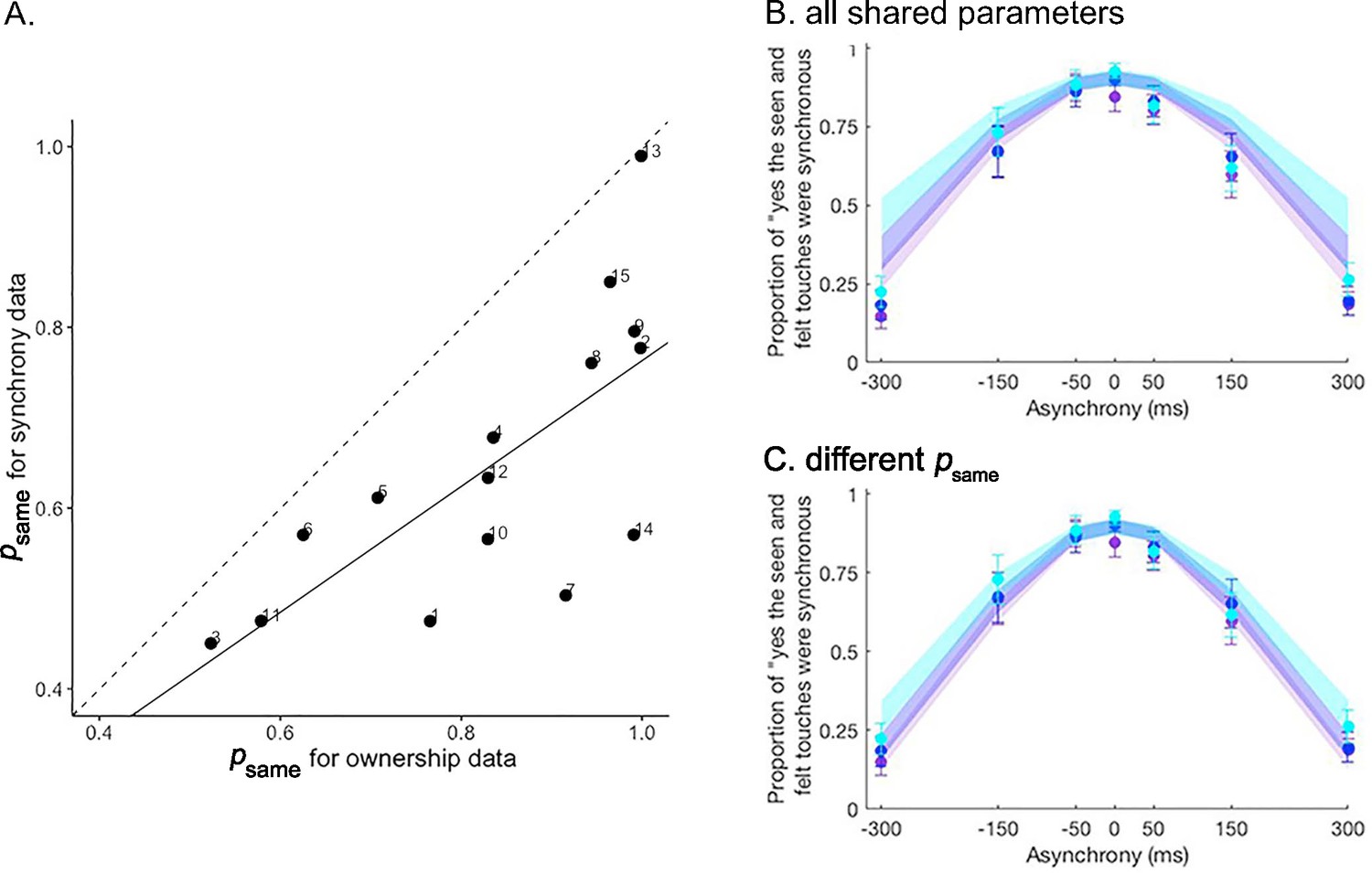
Extension analysis results.
(A) Correlation between the prior probability of a common cause estimated for the ownership and synchrony tasks in the extension analysis. The estimate is significantly lower for the synchrony task than for the ownership task. The solid line represents the linear regression between the two estimates, and the dashed line represents the identity. Numbers denote the participants’ numbers. (B and C) Colored dots represent the mean reported proportion of perceived synchrony for visual and tactile stimulation for each asynchrony under the 0 (purple), 30 (blue), and 50% (light blue) noise conditions (±SEM). Lighter shaded areas show the corresponding Bayesian causal inference (BCI) model predictions made when all parameters are shared between the ownership and synchrony data (B) and when is estimated separately for each dataset (C) for the different noise conditions (see also Figure 3—figure supplement 1).
-
Figure 3—source data 1
Parameter estimates for the extension and transfer analysis and collected answers in the synchrony detection tasks used in Figure 3.
- https://cdn.elifesciences.org/articles/77221/elife-77221-fig3-data1-v3.xlsx
Figure 3—figure supplement 1
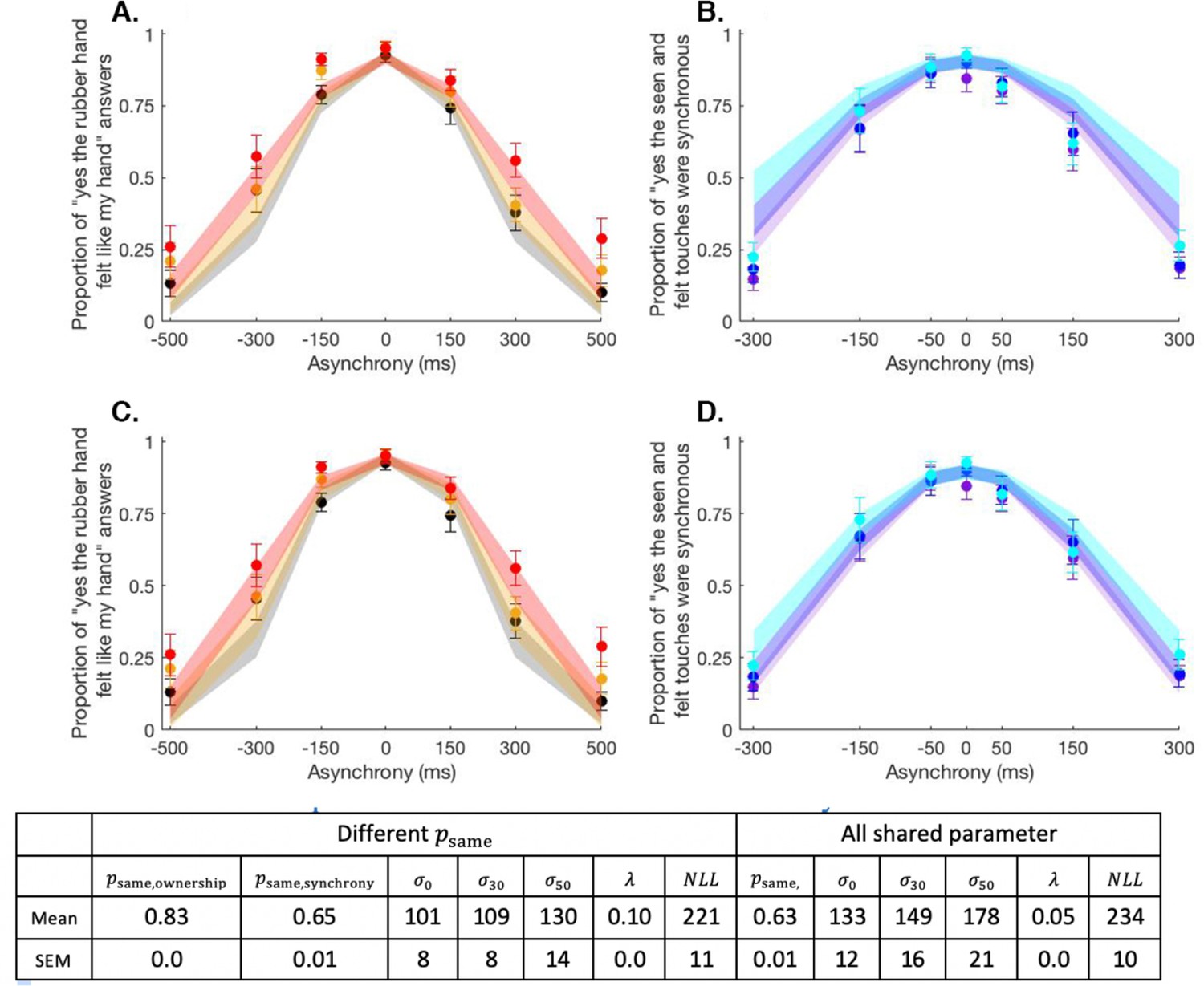
Mean + SEM behavioural (dots) and model (shaded areas) results for body ownership (A & C) and synchrony detection (B & D) tasks in the extension analysis.
The BCI model is fitted to the body ownership and synchrony data combined. Observed data for the 0% (black/purple dots), 30% (orange/dark blue dots), and 50% (red/light blue dots) of visual noise (body ownership/synchrony) and the corresponding predictions for the BCI model with a shared psame (A & B) and with distinct psame for each task (C & D). Below are the corresponding estimated parameters and negative log likelihood.
Figure 3—figure supplement 2

Mean + SEM behavioural (dots) and model (shaded areas) results for body ownership (A & C) and synchrony detection (B & D) tasks in the transfer analysis.
In this analysis, the body ownership task and the synchrony judgment task are compared by using the BCI model parameters estimated for one perception (ownership or synchrony) to predict the data from the other perception (synchrony or ownership). Observed data for the 0% (black/purple dots), 30% (orange/dark blue dots), and 50% (red/light blue dots) of visual noise (body ownership/synchrony) and the corresponding predictions for the BCI model with the same psame (full transfer; A & B) and with distinct psame for each task (partial transfer C & D). Below are the corresponding estimated parameters and negative log likelihood. "O to S" corresponds to the tting of synchrony data by the BCI model estimates from ownership data and "S to O" corresponds to the tting of ownership data by the BCI model estimates from synchrony data.
Figure 3—figure supplement 3
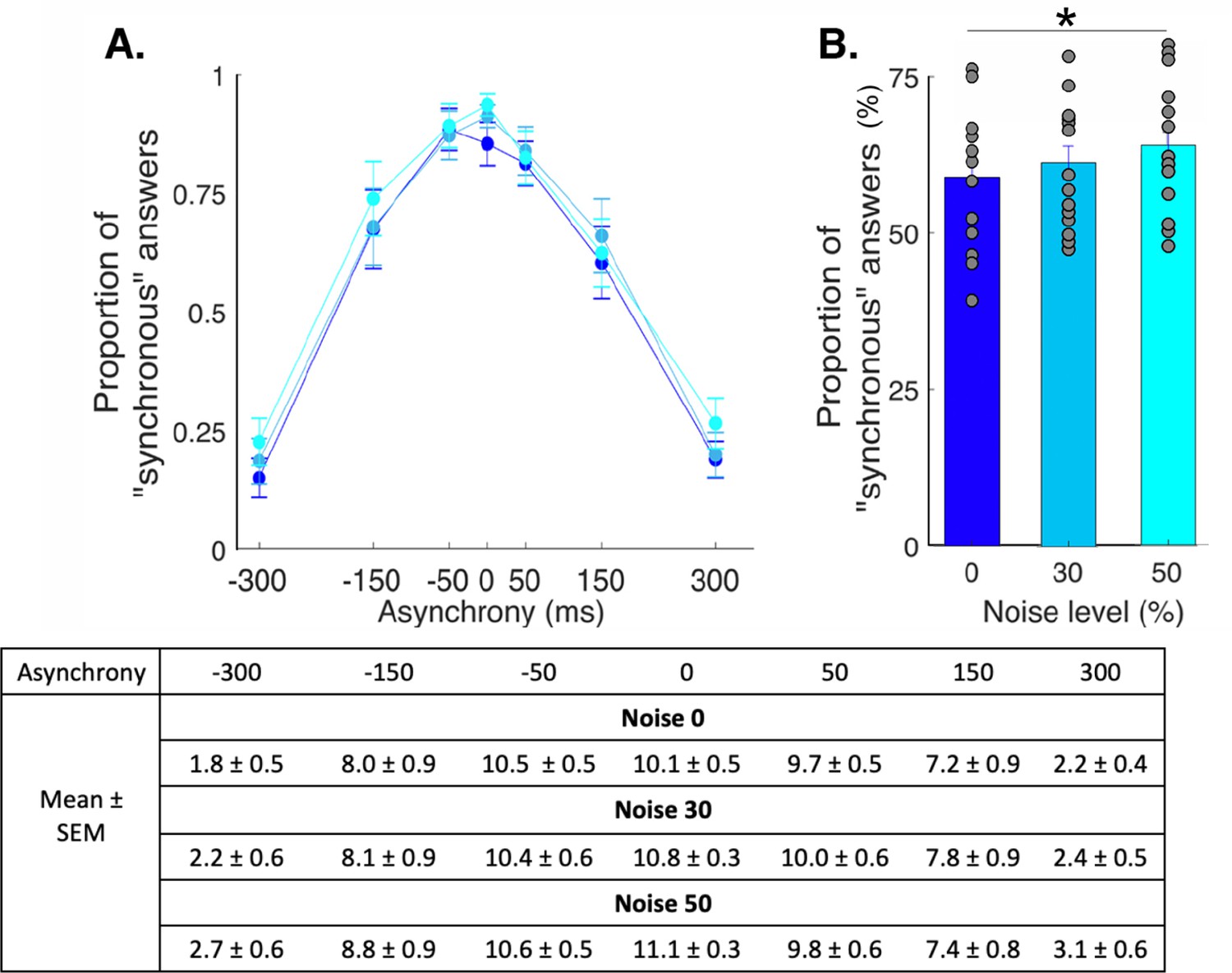
Perceived synchrony under different levels of visual noise.
(A) Colored dots represent the mean reported proportion of stimulation perceived as synchronous (+/-SEM) for each asynchrony for the 0% (dark blue), 30% (light blue), and 50% (cyan) noise conditions. (B) Bars represent how many times in the 84 trials the participants answered "yes [the touches I felt and the ones I saw were synchronous]' under the 0% (dark blue), 30% (light blue), and 50% (cyan) noise conditions. There was a significant increase in the number of `yes' answers when the visual noise increased * p < .05. The participants reported perceiving synchronous visuotactile taps in 89+/- 5% (mean +/- SEM) of the 12 trials when the visual and tactile stimulations were synchronous; more precisely, 85 +/- 4%, 90+/- 2%, and 93+/- 2% of responses were "yes" responses for the conditions with 0, 30, and 50% visual noise, respectively. When the rubber hand was touched 300 ms before the real hand, the taps were perceived as synchronous in 18+/- 5% of the 12 trials (noise level 0: 15+/- 4% noise level 30: 18+/- 5%, and noise level 50: 22+/- 5%); when the rubber hand was touched 300 ms after the real hand, visuotactile synchrony was reported in only 22+/- 5% of the 12 trials (noise level 0: 19+/- 4%, noise level 30: 20+/- 4%, and noise level 50: 26+/- 5%, main effect of asynchrony: F(6, 84) = 21.5, p <.001). Moreover, regardless of asynchrony, the participants perceived visuotactile synchrony more often when the level of visual noise increased but post-hoc tests showed that this di erence was only signi cant between the most extreme conditions of noise (F(2, 28) = 5.78, p = .008; Holmes' post hoc test: noise level 0 versus noise level 30: p = .30 davg = 0.2; noise level 30 versus noise level 50: p = .34, davg = 0.2; noise level 0 versus noise level 50: p = .01 davg = 0.4). The table below summa- rizes the mean (+/-SEM) the number of trials perceived as synchronous by the participants.
Figure 4 with 2 supplements
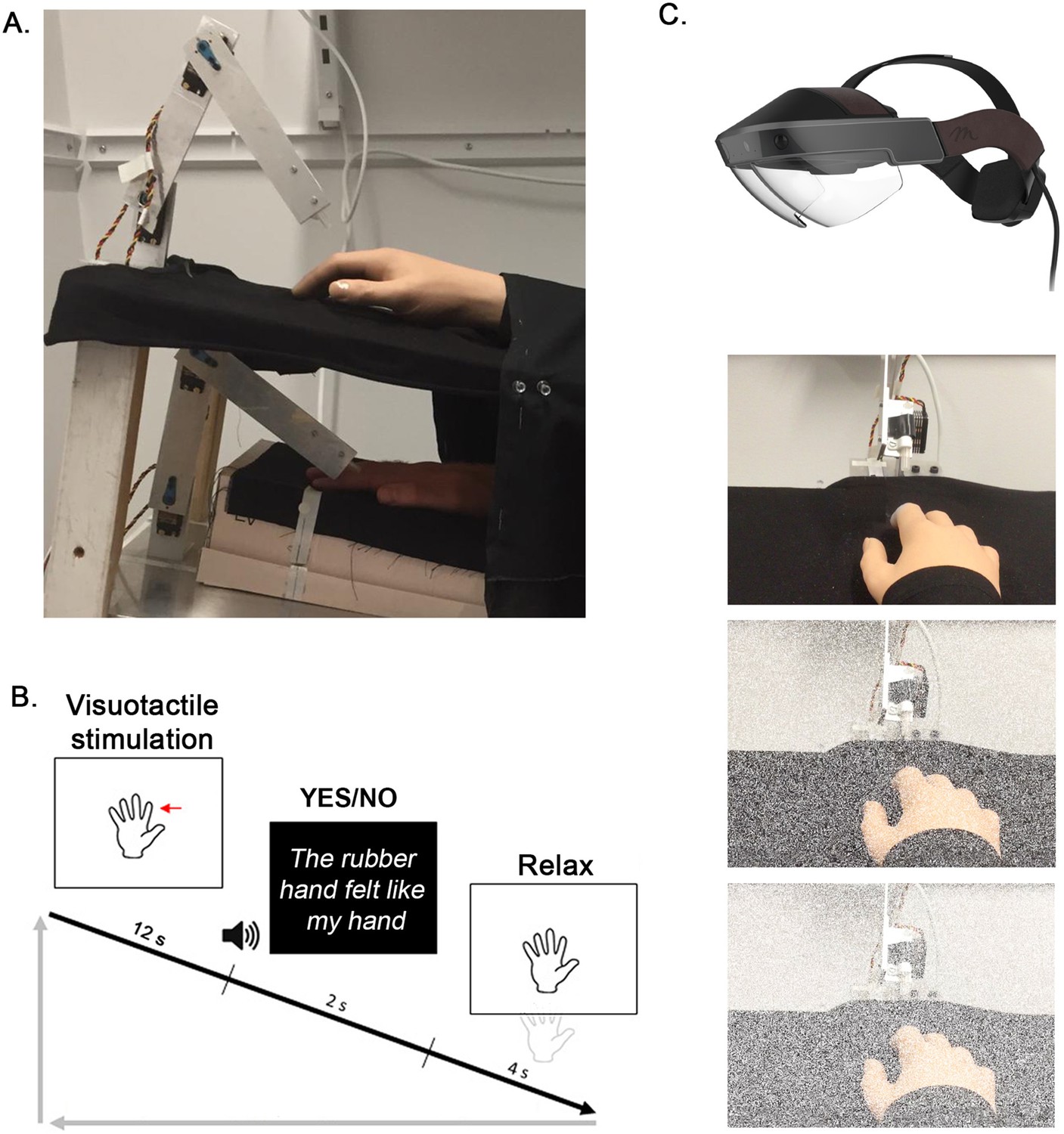
Experimental setup (A) and experimental procedure (B and C) for the ownership judgment task.
A participant’s real right hand is hidden under a table while they see a life-sized cosmetic prosthetic right hand (rubber hand) on the table (A). The rubber hand and real hand are touched by robots for periods of 12 s, either synchronously or with the rubber hand touched slightly earlier or later at a degree of asynchrony that is systematically manipulated (±150 ms, ±300 ms, or ± 500ms). The participant is then required to state whether the rubber hand felt like their own hand or not (‘yes’ or ‘no’ forced choice task) (B). Using the Meta2 headset, three noise conditions are tested: 0 (top picture), 30 (middle picture), and 50% (bottom picture) visual noise (C).
Figure 4—figure supplement 1
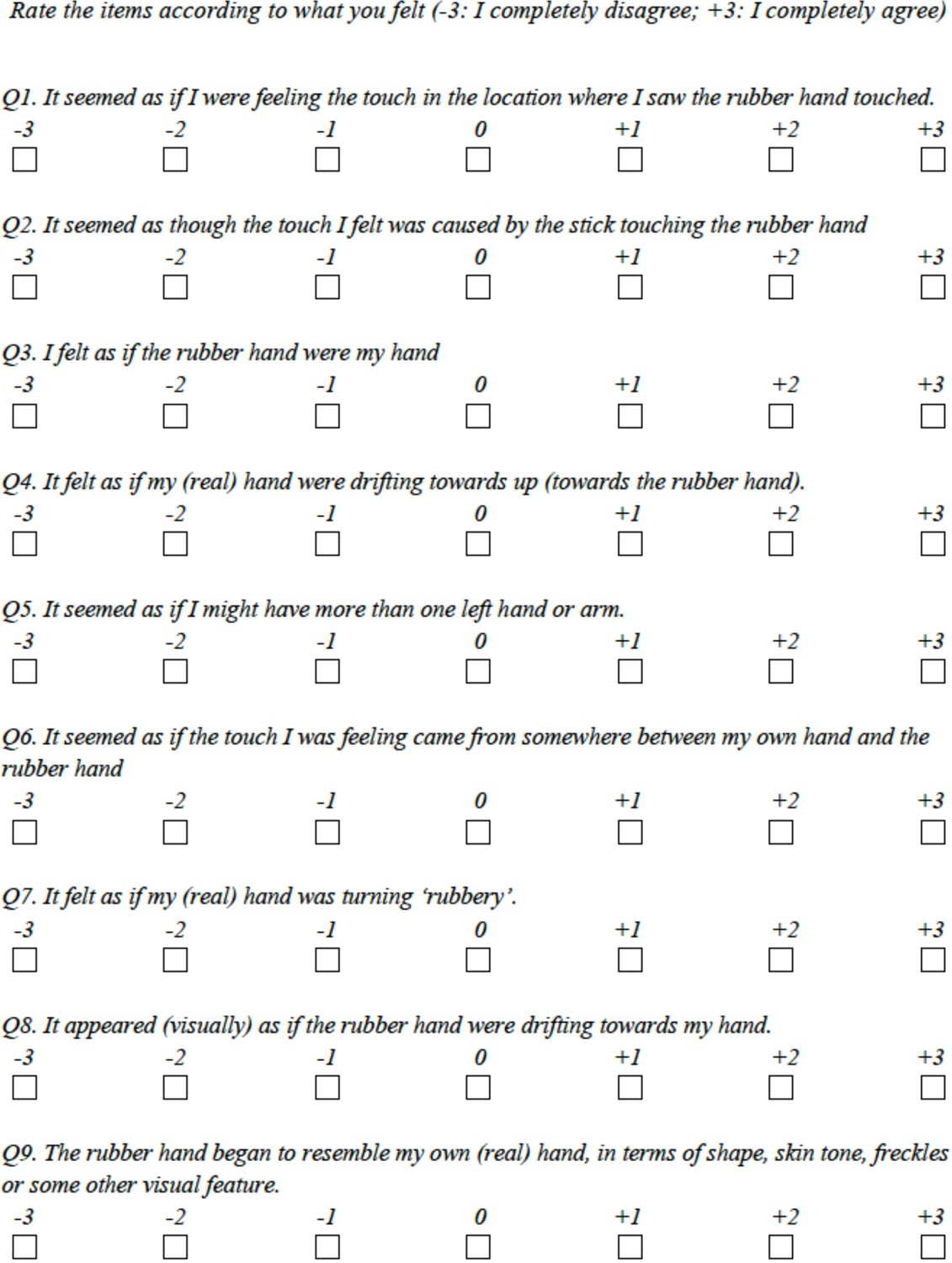
Questionnaire.
Figure 4—figure supplement 2

Mean questionnaire results for the participants included in the main experiment.
Figure 5
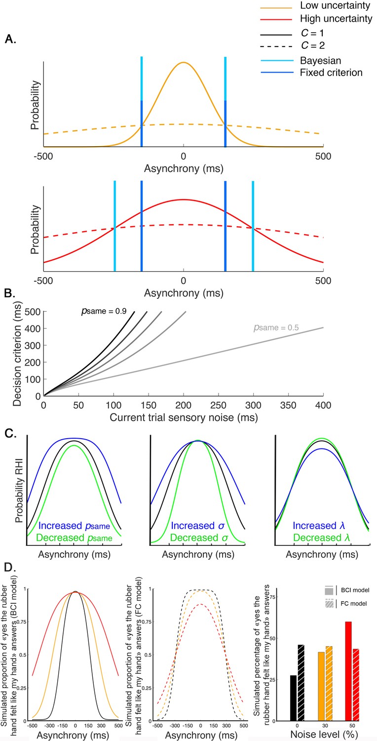
Decision process for the emergence of the rubber hand illusion (RHI) according to the Bayesian and fixed criterion observers.
(A) The measured asynchrony between the visual and tactile events for the low (orange) or high (red) noise level conditions and the probability of the different causal scenarios: the visual and tactile events come from one source, the observer’s body, or from two different sources. The probability of a common source is a narrow distribution (full curves), and the probability of two distinct sources is a broader distribution (dashed curve), both centered on synchronous stimulation (0 ms) such that when the stimuli are almost synchronous, it is likely that they come from the same source. When the variance of the measured stimulation increases from trial to trial, decision criteria may adjust optimally (Bayesian – light blue) or stay fixed (fixed – dark blue). The first assumption corresponds to the Bayesian causal inference (BCI) model, and the second corresponds to the fixed criterion (FC) model (see next paragraph for details). The displayed distributions are theoretical, and the BCI model’s psame is arbitrarily set at 0.5. (B) The decision criterion changes from trial to trial as a function of sensory uncertainty according to the optimal decision rule from the BCI model. Black curves represent this relationship for different psame values of 0.4–0.9 (from lightest to darkest). (C) From left to right, these last plots illustrate how the BCI model-predicted outcome is shaped by , , and , respectively. Left: = 0.8 (black), 0.6 (green), and 0.9 (blue). Middle: = 150 ms (black), 100 ms (green), and 200 ms (blue). Right: = 0.05 (black), 0.005 (green), and 0.2 (blue). (D) Finally, this last plot shows simulated outcomes predicted by the BCI model (in full lines and bars) and the FC model (in dashed lines and shredded bars). In this theoretical simulation, both models predict the same outcome distribution for one given level of sensory noise (0%); however, since the decision criterion of the BCI model is adjusted to the level of sensory uncertainty, an overall increase of the probability of emergence of the RHI is predicted by this Bayesian model. On the contrary, the FC model, which is a non-Bayesian model, predicts a neglectable effect of sensory uncertainty on the overall probability of emergence of the RHI.
Appendix 1—figure 1
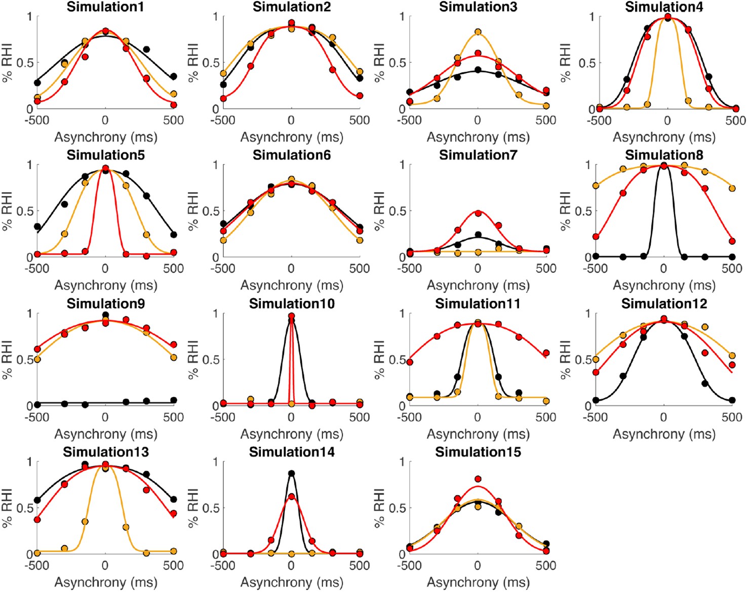
The figure displays simulated ‘yes (the rubber hand felt like my own hand)’ answers as a function of visuotactile asynchrony (dots) and corresponding Bayesian causal inference (BCI) model fit (curves).
As in the main text, black, orange, and red correspond to the 0, 30, and 50% noise levels, respectively.
Appendix 1—figure 2
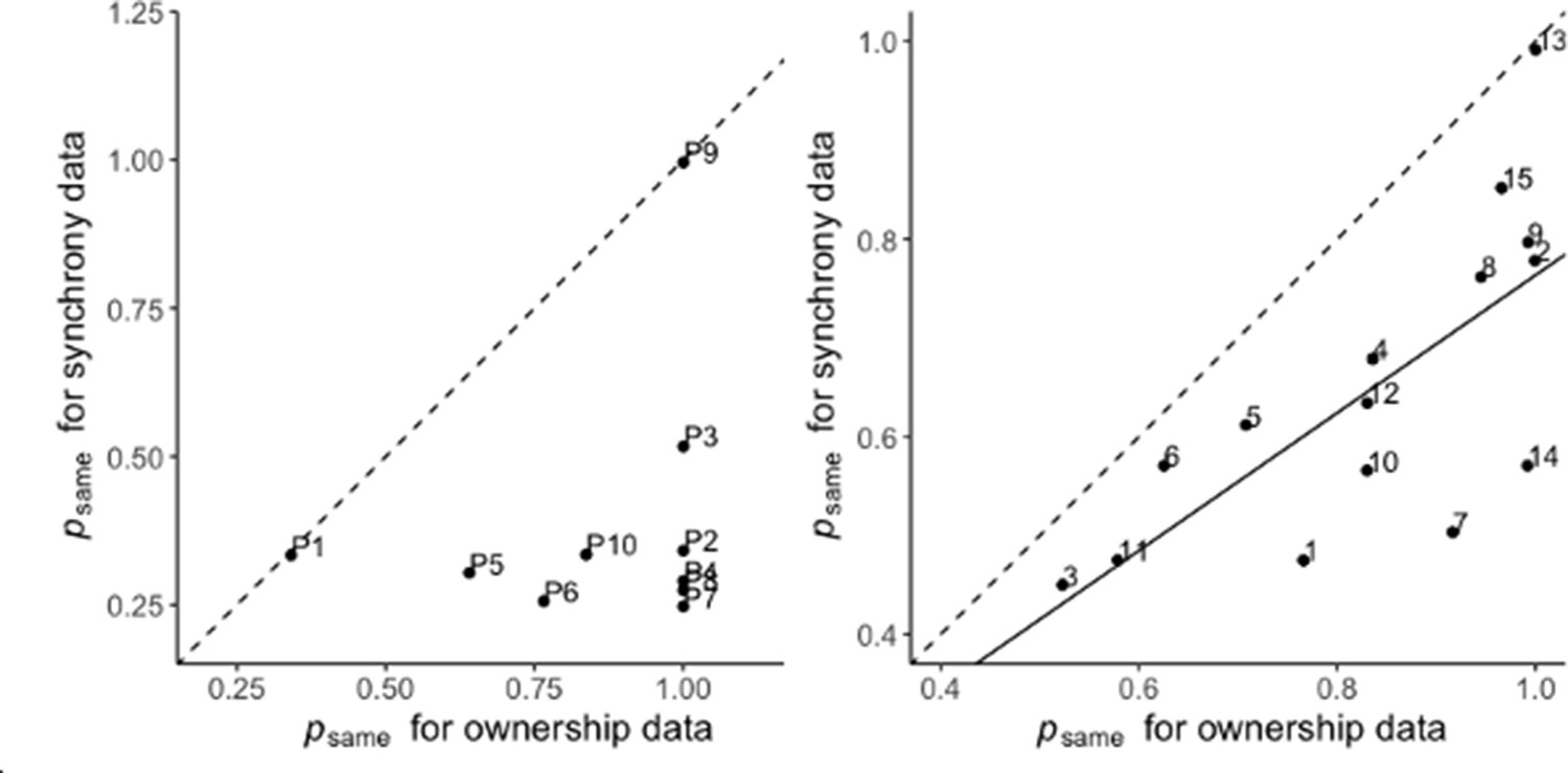
Correlation between the prior probability of a common cause psame estimated for the ownership and synchrony tasks in the extension analysis in the pilot study (left) and the main study (right).
The solid line represents the linear regression between the two estimates, and the dashed line represents the identity function (x=f[x]).
Author response image 1
Mixed-effect logistic regression with participant as random effect.
Dots represents individual responses, the curves are the regression fit, the shaded areas the 95% confidence interval.
Author response image 2
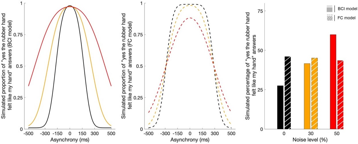
(D) Finally, this last plot shows simulated outcomes predicted by the Bayesian Causal Inference model (BCI in full lines and bars) and the fixed criterion model (FC in dashed lines and shredded bars).
In this theoretical simulation, both models predict the same outcome distribution for one given level of sensory noise (0%), however, since the decision criterion of the BCI model is adjusted to the level of sensory uncertainty, an overall increase of the probability of emergence of the rubber hand illusion is predicted by this Bayesian model. On the contrary, the FC model, which is a non- model, FC, predicts a neglectable effect of sensory uncertainty on the overall probability of emergence of the rubber hand illusion.
Author response image 3
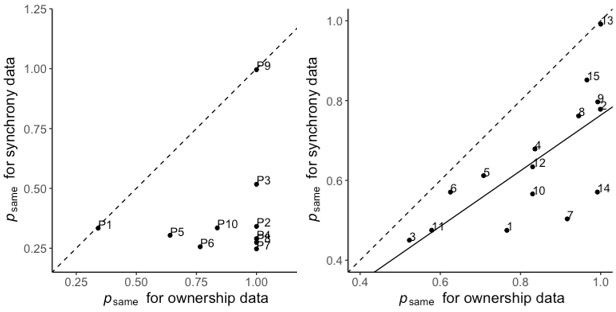
Correlation between the prior probability of a common cause estimated for the ownership and synchrony tasks in the extension analysis in the pilot study (left) and the main study (right).
The estimate is significantly lower for the synchrony task than for the ownership task. The solid line represents the linear regression between the two estimates, and the dashed line represents the identity function (x=f(x)).
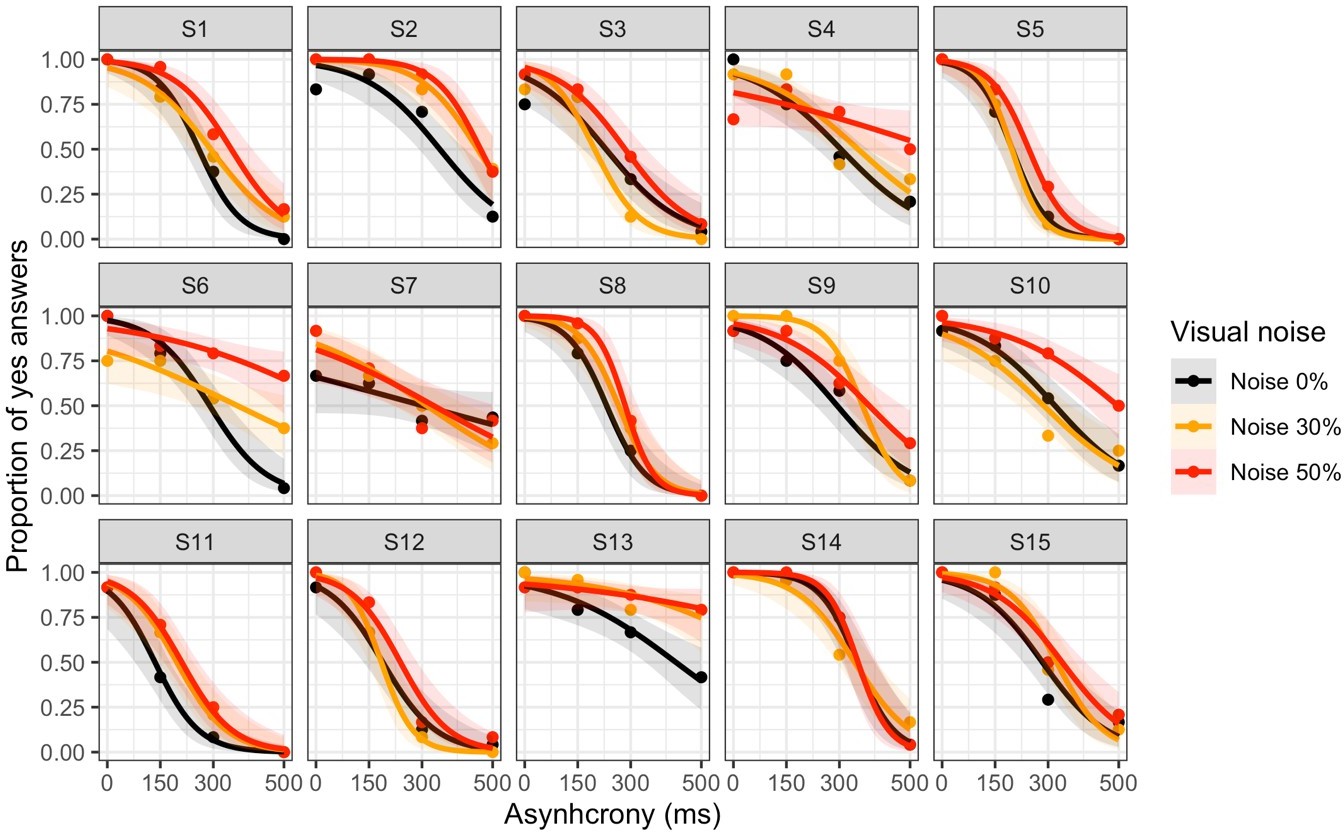
Author response image 4
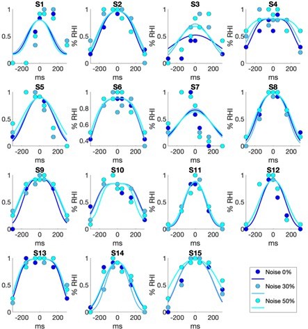
Individual data and BCI model fit.
The figure display one plot per participant, the “yes [the rubber hand felt like my own hand]" answers as a function of visuo-tactile asynchrony (dots) and corresponding BCI model fit (curves) are plotted. As in the main text, dark blue, light blue, and cyan correspond to the 0%, 30%, and 50% noise levels, respectively.
Tables
Table 1
Bootstrapped CIs (95% CI) of the Akaike information criterion (AIC) and Bayesian information criterion (BIC) differences between our main model Bayesian causal inference (BCI) and the BCI* (first line) and fixed criterion (FC; second line) models.
A negative value means that the BCI model is a better fit. Thus, the BCI model outperformed the other two.
| Model comparison | AIC (95% CI) | BIC (95% CI) | ||||
|---|---|---|---|---|---|---|
| Lower bound | Raw sum | Upper bound | Lower bound | Raw sum | Upper bound | |
| BCI – BCI* | –28 | –25 | –21 | –81 | –77 | –74 |
| BCI – FC | –116 | –65 | –17 | –116 | –65 | –17 |
-
Finally, the pseudo-R2 were of the same magnitude for each model (mean ± SEM: BCI = 0.62 ± 0.04, BCI* = 0.62 ± 0.04, FC = 0.60 ± 0.05). However, the exceedance probability analysis confirmed the superiority of the Bayesian models over the fixed criterian one for the ownership data (family exceedance probability [EP]: Bayesian: 0.99, FC: 0.0006; when comparing our main model to the FC: protected-EPFC = 0.13, protected-EPBCI = 0.87, posterior probabilities: RFX: p[H1|y] = 0.740, null: p[H0|y] = 0.260).
Table 2
Bootstrapped CIs (95% CI) for the Akaike information criterion (AIC) and Bayesian information criterion (BIC) differences between shared and different values for the Bayesian causal inference (BCI) model in the extension analysis.
A negative value means that the model with different values is a better fit.
| Model comparison | AIC (95% CI) | BIC (95% CI) | ||||
|---|---|---|---|---|---|---|
| Lower bound | Raw sum | Upper bound | Lower bound | Raw sum | Upper bound | |
| Different psame – shared parameters | –597 | –352 | –147 | –534 | –289 | –83 |
Table 3
Bootstrapped CIs (95% CIs) of the Akaike information criterion (AIC) and Bayesian information criterion (BIC) differences between the partial and full transfer analyses for the Bayesian causal inference (BCI) model.
‘O to S’ corresponds to the fitting of synchrony data by the BCI model estimates from ownership data. ‘S to O’ corresponds to the fitting of ownership data by the BCI model estimates from synchrony data. A negative value means that the partial transfer model is a better fit.
| Transfer direction | AIC (partial – full transfer, 95% CI) | BIC (partial – full transfer, 95% CI) | ||||
|---|---|---|---|---|---|---|
| Lower bound | Raw sum | Upper bound | Lower bound | Raw sum | Upper bound | |
| O to S | –1837 | –1051 | –441 | –1784 | –998 | –388 |
| S to O | –1903 | –1110 | –448 | –1851 | –1057 | –394 |
Appendix 1—table 1
Bounds used in the optimization algorithms.
| Parameter | Type | Hard bound | Plausible bound |
|---|---|---|---|
| Probability | (0, 1) | (0.3, 0.7) | |
| σ | Sensory noise (log) | (−Inf, +Inf) | (–3, 9) |
| λ | Lapse | (0, 1) | (eps, 0.2) |
| Asynchrony (log) | (−Inf, +Inf) | (–3, 9) |
Appendix 1—table 2
Initial parameters used to generate the simulations and recovered parameters.
| Participant | Initial | Recovered | ||||||||
|---|---|---|---|---|---|---|---|---|---|---|
| S1 | 0.53 | 246 | 164 | 129 | 0.09 | 0.51 | 264 | 176 | 133 | 0.11 |
| S2 | 0.74 | 183 | 204 | 130 | 0.15 | 0.86 | 152 | 171 | 109 | 0.21 |
| S3 | 0.39 | 281 | 96 | 223 | 0.15 | 0.41 | 313 | 111 | 251 | 0.09 |
| S4 | 0.90 | 97 | 32 | 85 | 0.02 | 0.89 | 94 | 33 | 83 | 0.02 |
| S5 | 0.73 | 185 | 96 | 29 | 0.07 | 0.74 | 176 | 101 | 31 | 0.07 |
| S6 | 0.54 | 238 | 198 | 215 | 0.19 | 0.50 | 294 | 221 | 275 | 0.00 |
| S7 | 0.26 | 138 | 275 | 110 | 0.12 | 0.27 | 151 | 17,803 | 123 | 0.12 |
| S8 | 0.90 | 1 | 240 | 141 | 0.01 | 0.87 | 25 | 256 | 146 | 0.01 |
| S9 | 0.69 | 7 | 265 | 296 | 0.08 | 0.66 | 0 | 274 | 316 | 0.06 |
| S10 | 0.19 | 10 | 142 | 12 | 0.05 | 0.36 | 36 | 4776 | 4 | 0.05 |
| S11 | 0.75 | 50 | 3 | 213 | 0.16 | 0.76 | 47 | 34 | 230 | 0.18 |
| S12 | 0.69 | 108 | 270 | 191 | 0.10 | 0.67 | 111 | 272 | 213 | 0.09 |
| S13 | 0.81 | 224 | 46 | 181 | 0.08 | 0.79 | 237 | 48 | 193 | 0.06 |
| S14 | 0.22 | 22 | 203 | 83 | 0.01 | 0.22 | 34 | 232 | 76 | 0.02 |
| S15 | 0.40 | 215 | 247 | 156 | 0.05 | 0.39 | 232 | 223 | 157 | 0.03 |
Appendix 1—table 3
Pilot data.
Number of ‘yes’ (the visual and tactile stimulation were synchronous) answers in the synchrony judgment task and of ‘yes’ (the rubber hand felt like it was my own hand) answers in the body ownership task (total number of trials per condition: 12).
| Participant | Synchrony judgment | Ownership judgment | ||||||||||||
|---|---|---|---|---|---|---|---|---|---|---|---|---|---|---|
| –500 | –300 | –150 | 0 | 150 | 300 | 500 | –500 | –300 | –150 | 0 | 150 | 300 | 500 | |
| P1 | 0 | 0 | 5 | 11 | 4 | 0 | 0 | 0 | 1 | 6 | 7 | 3 | 4 | 0 |
| P2 | 0 | 0 | 2 | 12 | 3 | 0 | 0 | 9 | 12 | 12 | 12 | 12 | 10 | 0 |
| P3 | 0 | 0 | 1 | 12 | 2 | 0 | 0 | 0 | 2 | 11 | 12 | 12 | 9 | 0 |
| P4 | 0 | 0 | 1 | 12 | 1 | 1 | 0 | 4 | 6 | 9 | 11 | 11 | 11 | 8 |
| P5 | 0 | 1 | 3 | 11 | 1 | 0 | 0 | 0 | 3 | 7 | 12 | 6 | 2 | 0 |
| P6 | 0 | 0 | 0 | 0 | 0 | 0 | 0 | 11 | 12 | 12 | 12 | 11 | 9 | 7 |
| P7 | 0 | 0 | 1 | 9 | 2 | 0 | 0 | 0 | 8 | 12 | 12 | 12 | 2 | 0 |
| P8 | 0 | 0 | 2 | 10 | 0 | 1 | 0 | 5 | 6 | 8 | 11 | 8 | 4 | 2 |
| P9 | 1 | 0 | 1 | 12 | 3 | 0 | 0 | 3 | 7 | 10 | 12 | 3 | 2 | 0 |
| P10 | 0 | 0 | 3 | 12 | 2 | 0 | 0 | 0 | 4 | 10 | 12 | 5 | 2 | 0 |
Additional files
Download links
A two-part list of links to download the article, or parts of the article, in various formats.
Downloads (link to download the article as PDF)
Open citations (links to open the citations from this article in various online reference manager services)
Cite this article (links to download the citations from this article in formats compatible with various reference manager tools)
Uncertainty-based inference of a common cause for body ownership
eLife 11:e77221.
https://doi.org/10.7554/eLife.77221


