Unfolding and identification of membrane proteins in situ
- International School for Advanced Studies, Italy
- Nano Life Science Institute, Kanazawa Medical University, Japan
- Department of Experimental and Clinical Medicine, Università Politecnica delle Marche, Italy
- Moleculaire Biofysica, Zernike Instituut, Rijksuniversiteit Groningen, University of Groningen, Netherlands
- The Abdus Salam International Centre for Theoretical Physics, Italy
- Institute of Materials (IOM-CNR), Area Science Park, Italy
- BioValley Systems & Solutions, Italy
Figures
Figure 1 with 9 supplements
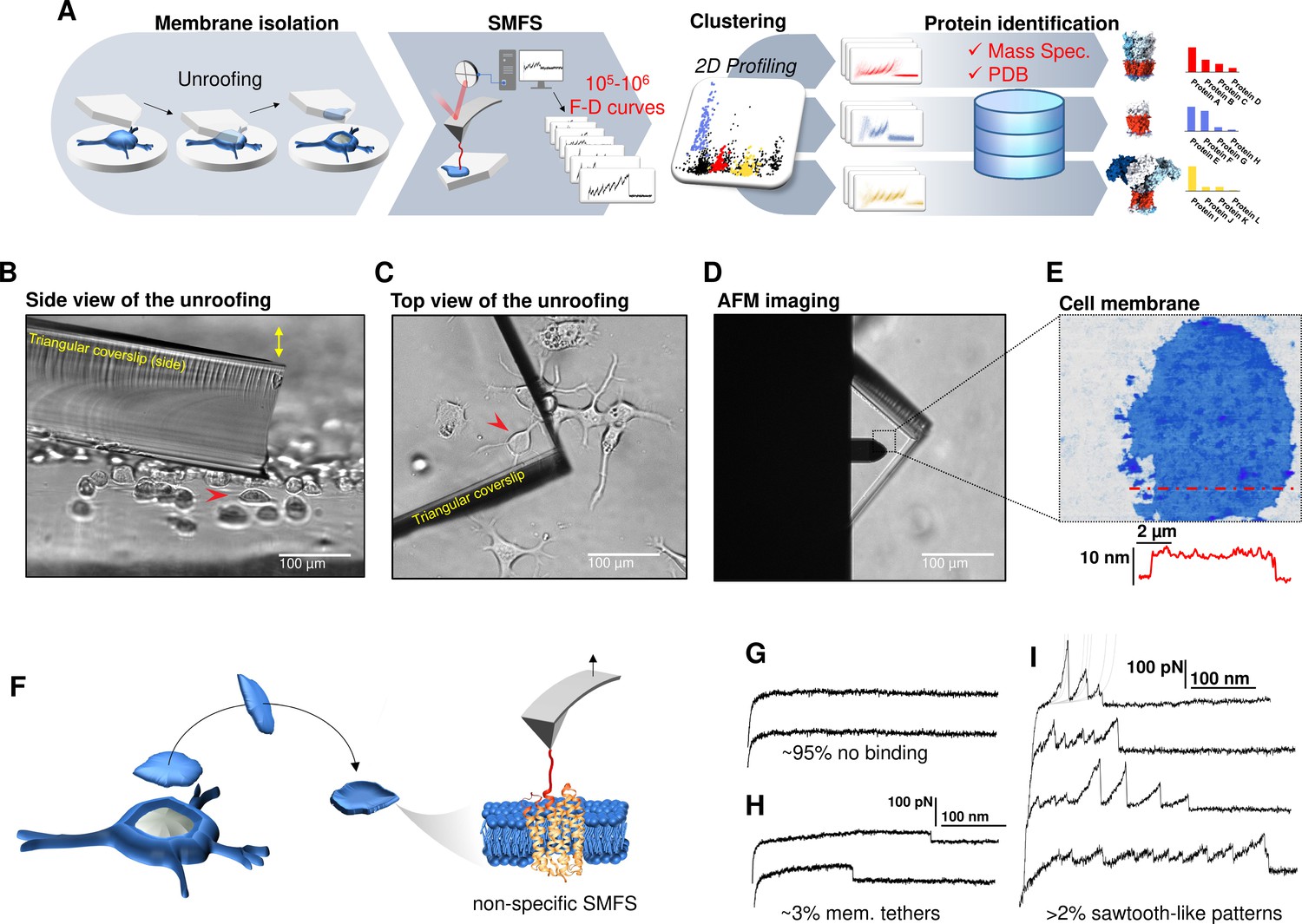
Experimental method for single-cell membrane isolation and protein unfolding.
(A) Workflow of the method in four steps: isolation of the apical membrane of single cells; atomic force microscopy (AFM)-based protein unfolding of native membrane proteins; identification of the persistent patterns of unfolding and characterization of the population of unfolding curves; Bayesian protein identification thanks to mass spectrometry data, Uniprot and PDB. (B) Side view and (C) top view of the cell culture and the triangular coverslip approaching the target cell (red arrow) to be unroofed. (D) Positioning of the AFM tip in the region of unroofing. (E) AFM topography of the isolated cell membrane with profile. (F) Cartoon of the process that leads to single-molecule force spectroscopy (SMFS) on native membranes. Examples of force-distance (F-D) curves of (G) no binding events; (H) constant viscous force produced by membrane tethers during retraction; (I) sawtooth-like patterns, typical sign of the unfolding of a membrane protein.
Figure 1—figure supplement 1
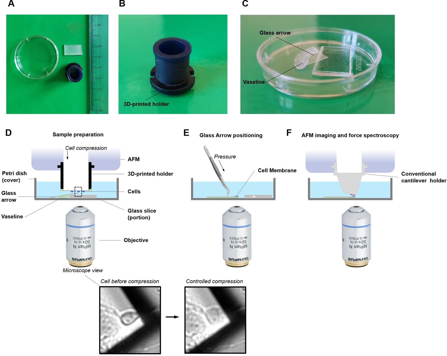
Schematic setup for single-cell unroofing.
(A) Example of the tools used for unroofing. A custom-made 3D-printed holder, glass stand, glass arrow, and Petri dish were shown here along with a ruler in centimeter scale. (B) The side view of the 3D-printed holder. (C) Closed view of sample container. The Vaseline was put along the boundary of the glass stand and the glass arrow, and then put them sequentially into a Petri dish which served as a sample container. In this way, this glass arrow would be tilted at about 30 degrees. (D) Details of the whole apparatus. The sample container was positioned on the atomic force microscopy (AFM) sample stage and added 4 ml Ringer’s buffer. The coverslip with cultured cells was mounted upside down on the 3D-printed holder using Vaseline. Then the 3D-printed holder was installed into the AFM head. The cells on the coverslip were brought to contact with the top corner of glass arrow via decreasing the height of AFM head and this process was monitored by optical microscope. The more detail of squeezing the cell and cell membrane unroofing, please refer to Galvanetto, 2018a, and for applications (Galvanetto, 2020). (E) After isolation of the cell membrane, the glass arrow was glued with the Vaseline already underneath making sure that no bubble was present in the sample area. (F) The presence of the membrane is confirmed by AFM in a tapping mode and then single-molecule force spectroscopy (SMFS) experiments can be performed.
Figure 1—figure supplement 2
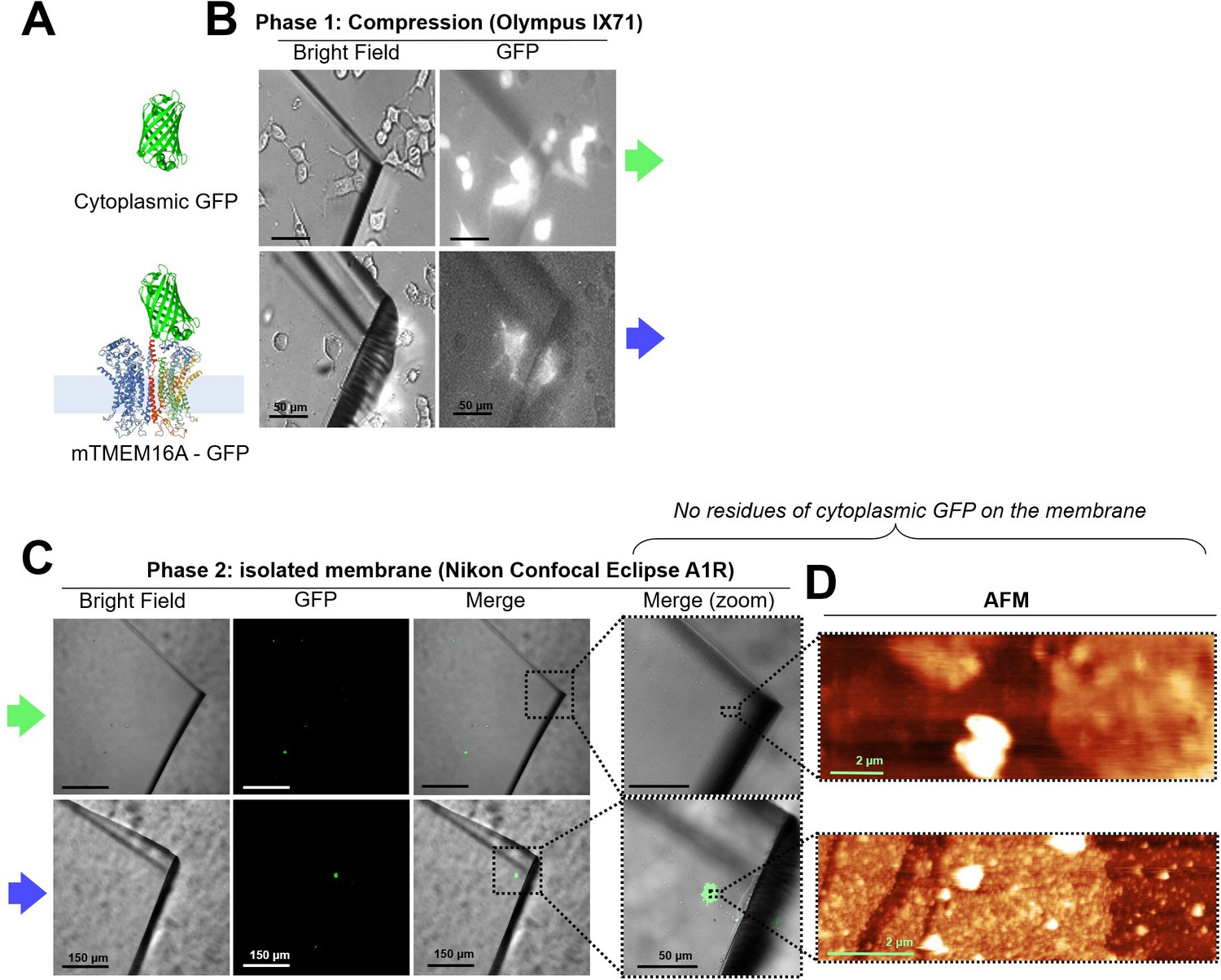
In NG108-15 cells, membrane proteins remain into the membrane after unroofing, while cytoplasmic proteins do not.
(A) (Top) Cytoplasmic GFP and (bottom) mTMEM16A-GFP overexpressed in NG108-15 cells. (B) Bright-field and fluorescence images taken during the compression on the inverted microscope-atomic force microscopy (AFM) system. (C) Images taken with a confocal microscope of the coverslip quarter after unroofing; the rough surface under the glass is due to the Vaseline layer used to fix the coverslip quarter. No residues of cytoplasmic GFP are found in the top row. (D) AFM images of the area in the right-most panel of (C) showing the presence of membrane patches in both the samples.
Figure 1—figure supplement 3
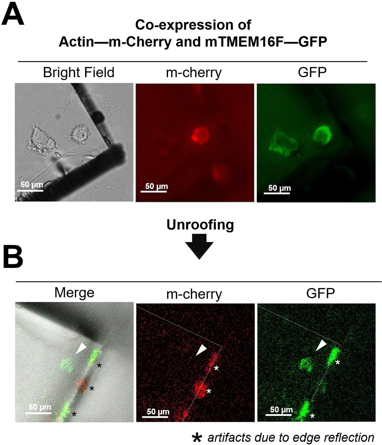
Absence of cytoplasmic proteins after unroofing of NG108-15 cells.
(A) Before unroofing. From left to right: bright-field image showing a piece of glass over a neuroblastoma cells transfected with actin labeled with mCherry-Lifeact-7 and the membrane protein TMEM16F tagged with GFP; in the center an image of the red fluorescence emitted by the labeled actin; in the right an image of the green fluorescence emitted by the TMEM16F-GFP. (B) After unroofing only the green signal from TMEM16F is detected (right panel) and no red fluorescence is observed (center panel and the location indicated by the white arrowhead). * (asterisks) indicate the fluorescence due to edge reflections. The green signal is detected exactly where the neuroblastoma cell was located (left panel).
Figure 1—figure supplement 4
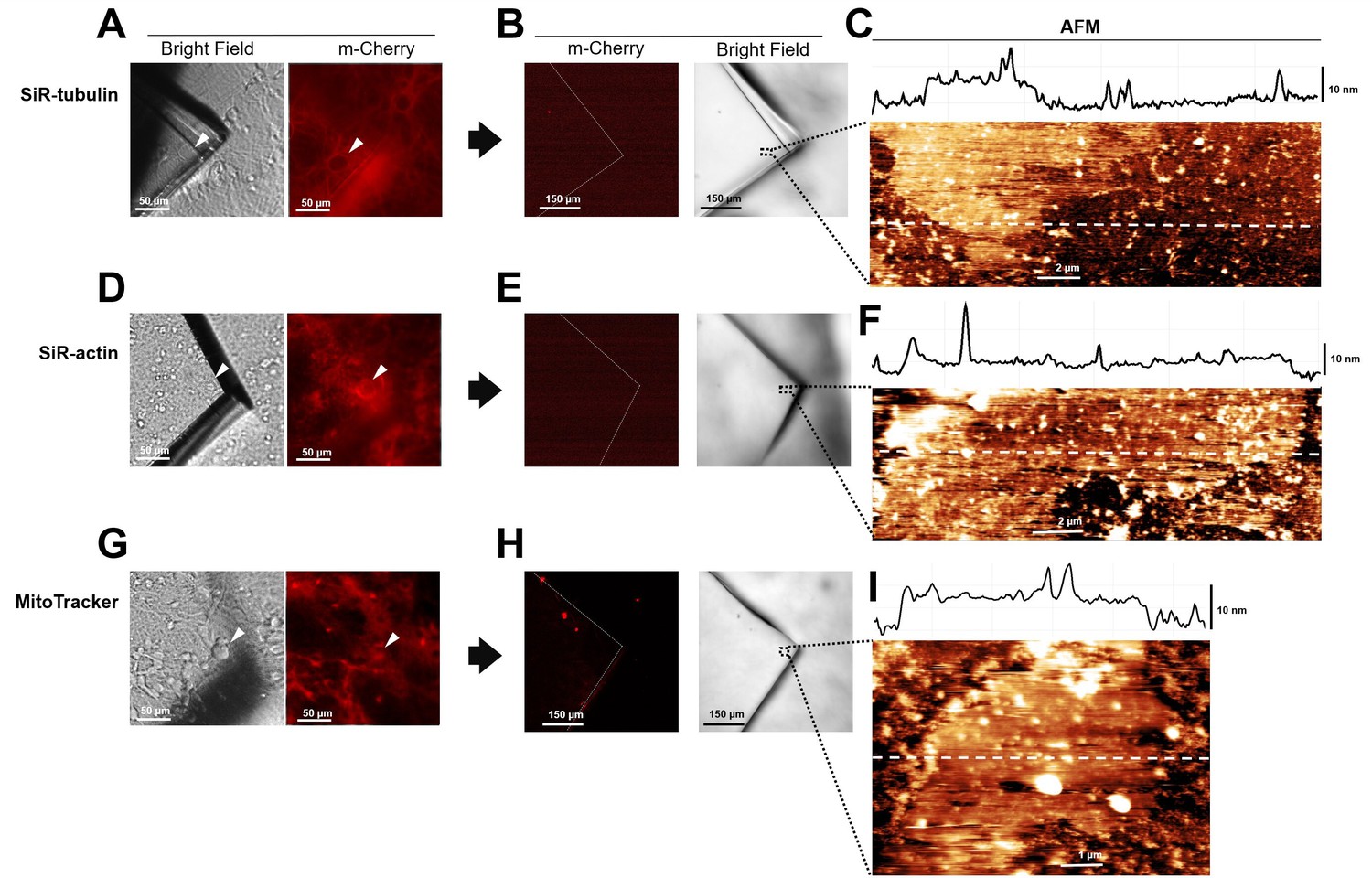
Absence of cytoplasmic proteins in unroofed membranes in hippocampal cells.
(A) Before unroofing. Bright-field image of the piece of glass over a neuroblastoma cell. Red fluorescence emitted by SiR-tubulin. (B) After unroofing. No red fluorescent signal detected. (C) Atomic force microscopy (AFM) imaging of region indicated in (B) showing the presence of a piece of membrane. (D, E, and F) As in (A, B, and C) but for Sir-Actin. (G, H, and I) As in (A, B, and C) but for Mito Tracker labeling mitochondria.
Figure 1—figure supplement 5
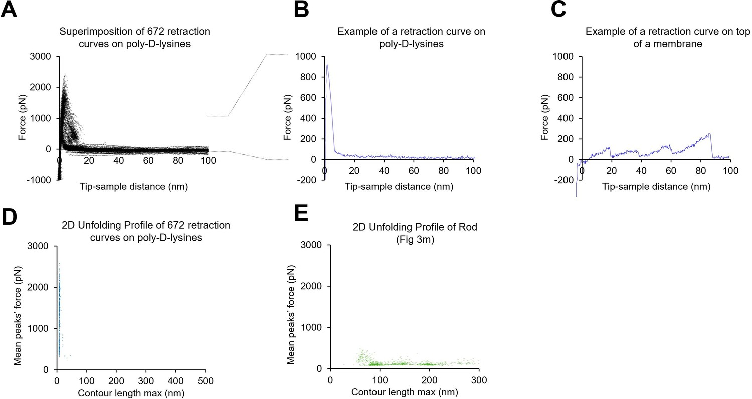
Absence of poly-D-lysine contamination in the single-molecule force spectroscopy (SMFS) data from unroofed cell membranes.
(A) 672 force-distance (F-D) curves obtained from a coverslip just coated with poly-D-lysine and in the absence of any cell. (B) Example of one F-D curve from A. (C) One example of an F-D curve obtained in the presence of a biological membrane. (D) Plot of the mean force against maximum contour length of the traces obtained from the experiment shown in A; (E) as in (D) but for F-D curves obtained from rod membranes. For the transformation tip-sample-separation to contour length we solved the worm-like chain (WLC) model (Ainavarapu et al., 2007): for . Here, is the persistence length of the protein (0.4 nm), is the tip-sample-separation of one point is the measured force. is the contour length point of the transformed point.
Figure 1—figure supplement 6
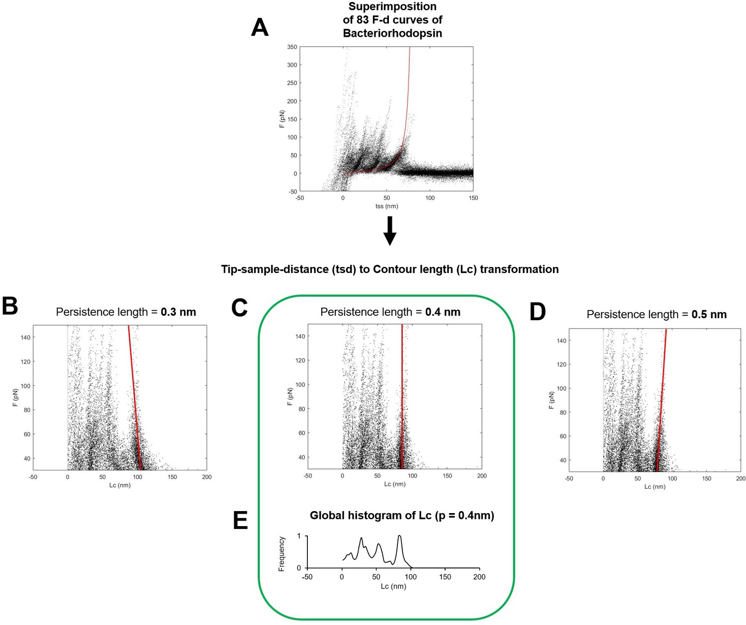
Determination of the optimal persistence length of the detachment peak used for the total contour length calculation (Lcmax).
(A) Superimposition of 83 force-distance (F-D) curves of Bacteriorhodopsin (the red line is the worm-like chain curve with persistence length = 0.4 nm and contour length = 85 nm). (B, C, D) Transformation of the ordinates of the points in (A) to the contour length space (Lc) with persistence length of 0.3 nm in (B), 0.4 in (C), and 0.5 in (D). Solid red lines indicate the best fit of the points belonging to the last unfolding peak: 0.4 nm of persistence length is the correct/optimal value because in the contour length space, the force points representing the unfolding of the polymer with a constant contour length must lay on a vertical line. (D) Global histogram of contour length of (C).
Figure 1—figure supplement 7

Membrane proteins architectures.
(A) Eight classes of membrane proteins and their fraction obtained from data present in the PDB-OPM. (B) Distribution of the position of the C and N termini relative to the center of the cell membrane along the axis perpendicular to the membrane. (C) Cartoon representing the complete unfolding of a membrane protein and its force-distance (F-D) curve. (D) Simultaneous unfolding of two proteins and the resulting involved force which is the arithmetic sum of the one necessary to unfold one protein and the other. (E) Incomplete unfolding of a protein leads to a similar but shorter unfolding curve. (F) Unfolding from a cytoplasmic loop. (G) Idealized decomposition of F-D curves of a multiple unfolding/unfolding from a loop. Effective F-D curves are affected by multiple binding: If one of the two protein is short, the unfolding of the longer one can still be recognized although it will differ in the intersection part. If one protein unfolds with lower forces than the other, still the pattern of the second one can be recognized, but it will be noisy.
Figure 1—figure supplement 8
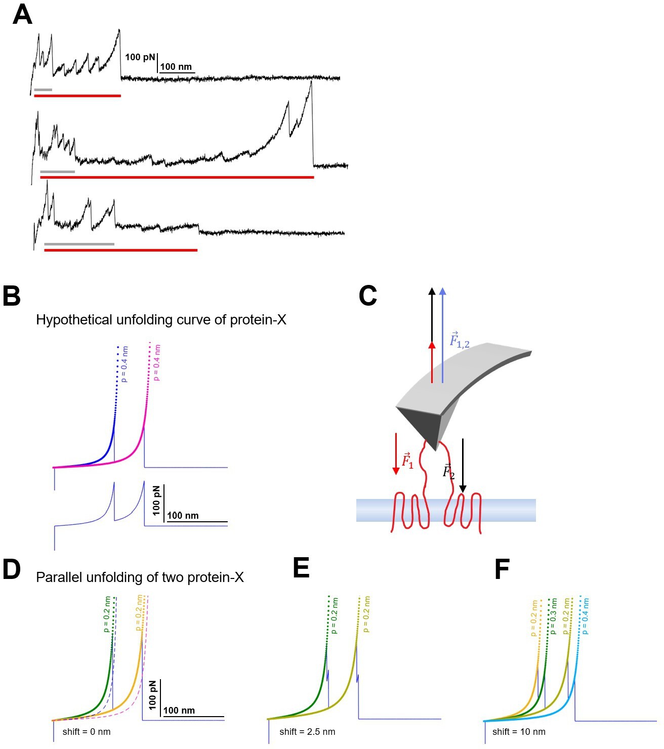
Candidates of multiple unfolding and origin of persistence length deviation.
(A) Observed force-distance (F-D) curves showing the features of multiple unfolding events (red horizontal bar: long protein, gray horizontal bar: short protein; guessed). (B) Hypothetical unfolding curve of protein-X (peak 1: Lc = 100 nm, F=150 pN; peak 2: Lc = 150 nm, F=150 pN) fitted with the worm-like chain (WLC) model with standard persistence length P=0.4 nm. (C) The force applied by the atomic force microscopy (AFM) tip balances the unfolding forces of the two proteins during the retraction. (D) The effective F-D curve recorded during parallel unfolding of two protein-X corresponds to the sum of a single unfolding curve (B) and it is best fitted with half the persistence length P=0.2 nm. (E) Relative shift of 2.5 nm and (F) 10 nm still result in deviations of the measured persistence length and display the doubling of the peaks.
Figure 1—figure supplement 9

Clustering.
(A) Block scheme of the clustering method. (B) Area of similarity (AoS) for cluster R1 used for block 5 described in Methods. (C) Plot of the scores generated by the AoS on (B) of the force-distance (F-D) curves in the Dataset Rod filtered by length in the descending order. (D) Table showing the number of clusters that was merged to form the final selection of Figure 3.
Figure 2 with 3 supplements
Unfolding of reconstituted mixtures of membrane proteins.
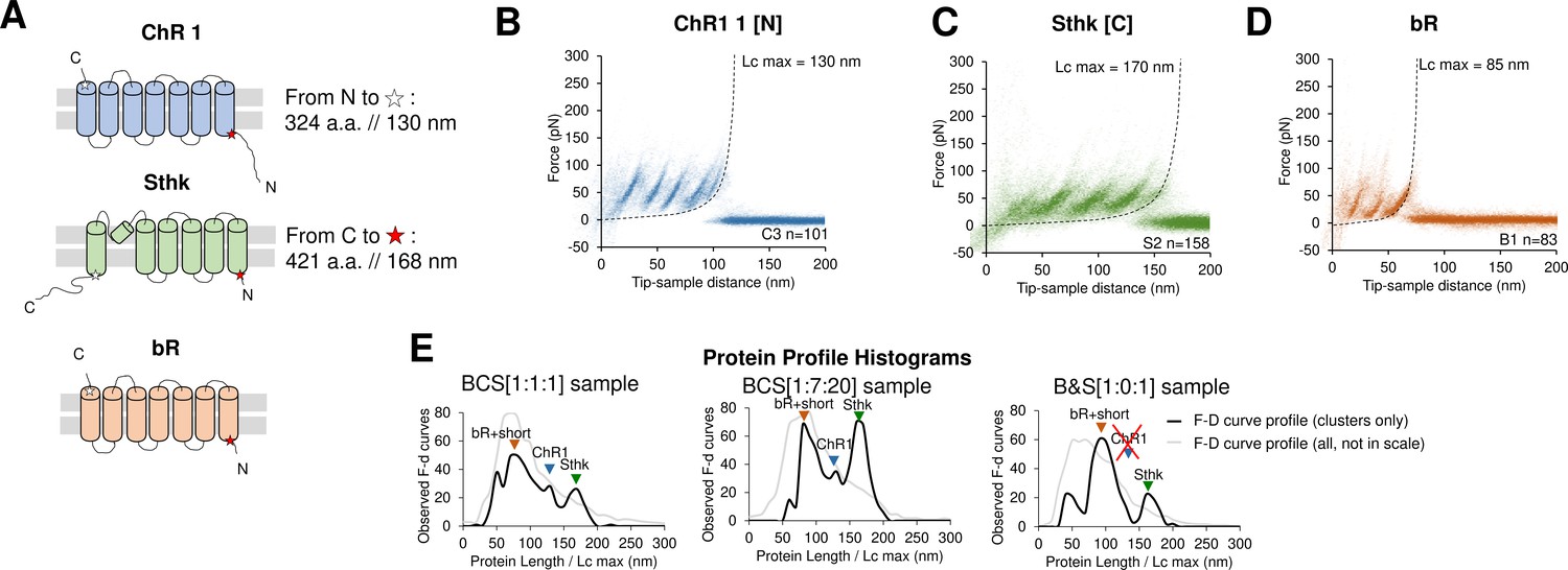
(A) Scheme of the structure of the three purified proteins used in the in vitro preliminary step: Channelrhodopsin (ChR1), SthK, and Bacteriorhodopsin (bR) (cylinders represent α-helices). (B) Superimposition of 101 unfolding curves (density plot) of the full unfolding of ChR1 from the N-terminus. (C) Density plot of the full unfolding of Sthk from the C-terminus. (D) Density plot of the full unfolding of bR. (E) Protein profile, that is, the histogram of the maximal contour length (Lcmax) of all the force-distance (F-D) curves in the clusters (black line), and of all the F-D curves collected from the sample (gray line, not in scale), from samples with mixtures of bR, ChR1, and SthK with a relative abundance of 1:1:1, 1:7:20, and 1:0:1 (bR-SthK only). Arrows indicate where the F-D curves of (B), (C), and (D) accumulate in the histogram. The peak at ~90 nm indicated by bR+short also contains the shorter clusters of ChR1 and SthK shown in Figure 2—figure supplement 1, which also appear in the mixtures.
Figure 2—figure supplement 1

Unfolding of reconstituted membrane proteins.
(A) Scheme of the structure of the three purified proteins used in the in vitro preliminary step: Channelrhodopsin (ChR1), SthK, and Bacteriorhodopsin (bR) (cylinders represent α-helices). (B) Geometrical length of the amino acid chains constituting the whole protein, the C- and N-terminals and of the length of the whole protein minus the C- and N-terminal. The codes in red represent the name and the respective unfolding cluster. (C) Clusters obtained from a dataset of n=18,868 traces from a sample with ChR1. The histogram bars on the right of each density plot represent the Bayesian assignment according to our procedure (described in Methods). [N] and [C] stand for ‘protein unfolded from N-terminus/C-terminus’. Below each density plot the corresponding global histogram of contour length showing the most likely position for the unfolding peaks to occur: the circles with numbers are then reported in (A) to show the position of the preferential unfolding position in the structure. (D) Clusters obtained from a dataset of n=115,155 traces from a sample with SthK. (E) Clusters obtained from a dataset of n=35,599 traces from a sample with bR.
Figure 2—figure supplement 2

In vitro experiments with co-reconstitution of SthK and Channelrhodopsin (ChR1) (relative concentration 1:1) showing the five clusters obtained, and comparison of these new patterns S&Cx to the previous Cx and Sx clusters from single reconstitution.
(A–E) Clusters (called S&C1, …, S&C5) resulting from the simultaneous reconstitution of ChR1 and SthK in a concentration ratio of 1:1, and global histogram of the contour length comparison with the best candidate obtained from the single reconstitution (from Figure 2—figure supplement 1). Bayesian probability shown on the right of each cluster. For (C) and (D) we report the improvement in the Bayesian identification when the structure of the protein is taken into account (see Methods Bayesian estimation). (F) Black line: distribution of the maximum of the contour length (Lcmax) of force-distance (F-D) curves of the clusters (except (A)) obtained in the co-reconstituted sample; blue and green bars: real length of the protein in the sample.
Figure 2—figure supplement 3

Clusters obtained in in vitro experiments with mixtures of Bacteriorhodopsin (bR), Channelrhodopsin (ChR1), and Sthk at different relative concentrations [1:1:1] and [1:7:20].
Cluster names: BCS[1:1:1]x and BCS[1:7:20]x. (A) Candidates’ prediction of the clusters obtained in samples with bR, ChR1, and SthK and relative abundance of [1:1:1]. (The number in gray indicates the total contour length of the clusters called Lcmax, the number in blue the number of traces per cluster.) (B) Same as (A) for relative abundance of [1:7:20].
Figure 3 with 1 supplement
Unfolding clusters in native cell membranes.
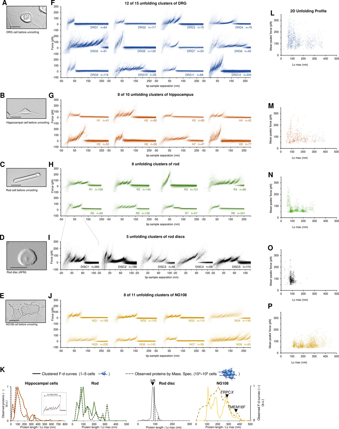
Bright-field image of (A) dorsal root ganglia neuron; (B) hippocampal neuron; (C) rod before unroofing (scale bar 15 µm). (D) Atomic force microscopy (AFM) error image of an isolated disc (scale bar 1 µm), (E) NG108-15 cells. (F, G, H, I, J) Examples of obtained clusters from the native membranes shown as density plots, that is, superposition of the n unfolding curves agglomerated and colored as a heatmap. (K) Comparison of the protein profiles obtained with mass spectrometry vs. the force-distance (F-D) curves obtained with single-molecule force spectroscopy (SMFS) shows a good correlation. The protein profile from mass spectrometry is the normalized histogram of the total number of proteins found in the sample, considering their abundance. The protein profile from SMFS is the histogram of the maximal contour length (Lcmax) of all the F-D curves selected with our clustering procedure. (L, M, N, O, P) Representation of all the clustered F-D curves in 2D: x-axis is the maximum contour length; y-axis is the average unfolding force (DRG: n=1255; hippocampus: n=563; rod: n=1039; disc: n=703, NG108-15 cells: n=1591).
Figure 3—figure supplement 1
Alternative visualizations of cluster analysis.
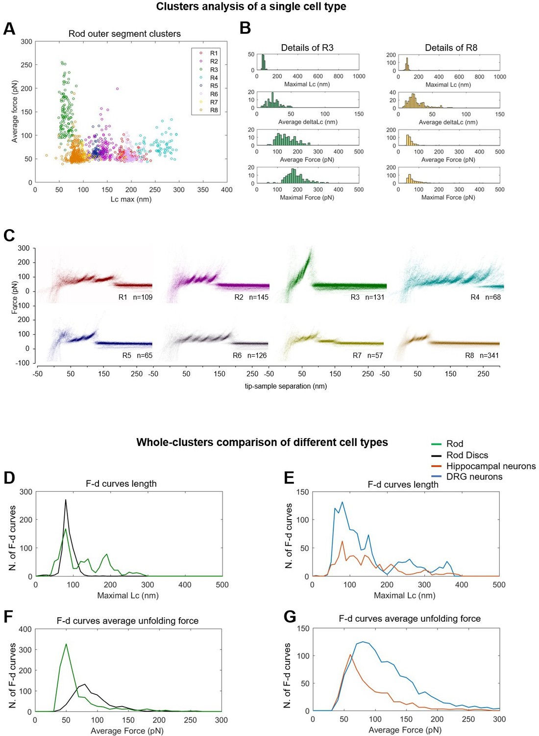
(Top) Two-dimensional unfolding profile in the compact representation of all the clustered force-distance (F-D) curves: x-axis is the maximum contour length; y-axis is the average unfolding force (DRG: n=1255; hippocampus: n=563; rod: n=1039; disc: n=703, NG108: n=1591). (A) Plot of all the F-D curves belonging to the clusters of the rod outer segment plotted with different colors in the ‘average unfolding force’ vs. ‘maximal contour length’ space. (B) Distribution of representative observables for clusters R3 and R8. (C) Density plots of clusters in (A). Comparison of the maximal contour length profiles (D and E) and of the average unfolding forces (F and G) of the four cell types investigated.
Figure 4 with 1 supplement
Bayesian identification and conditional probabilities.
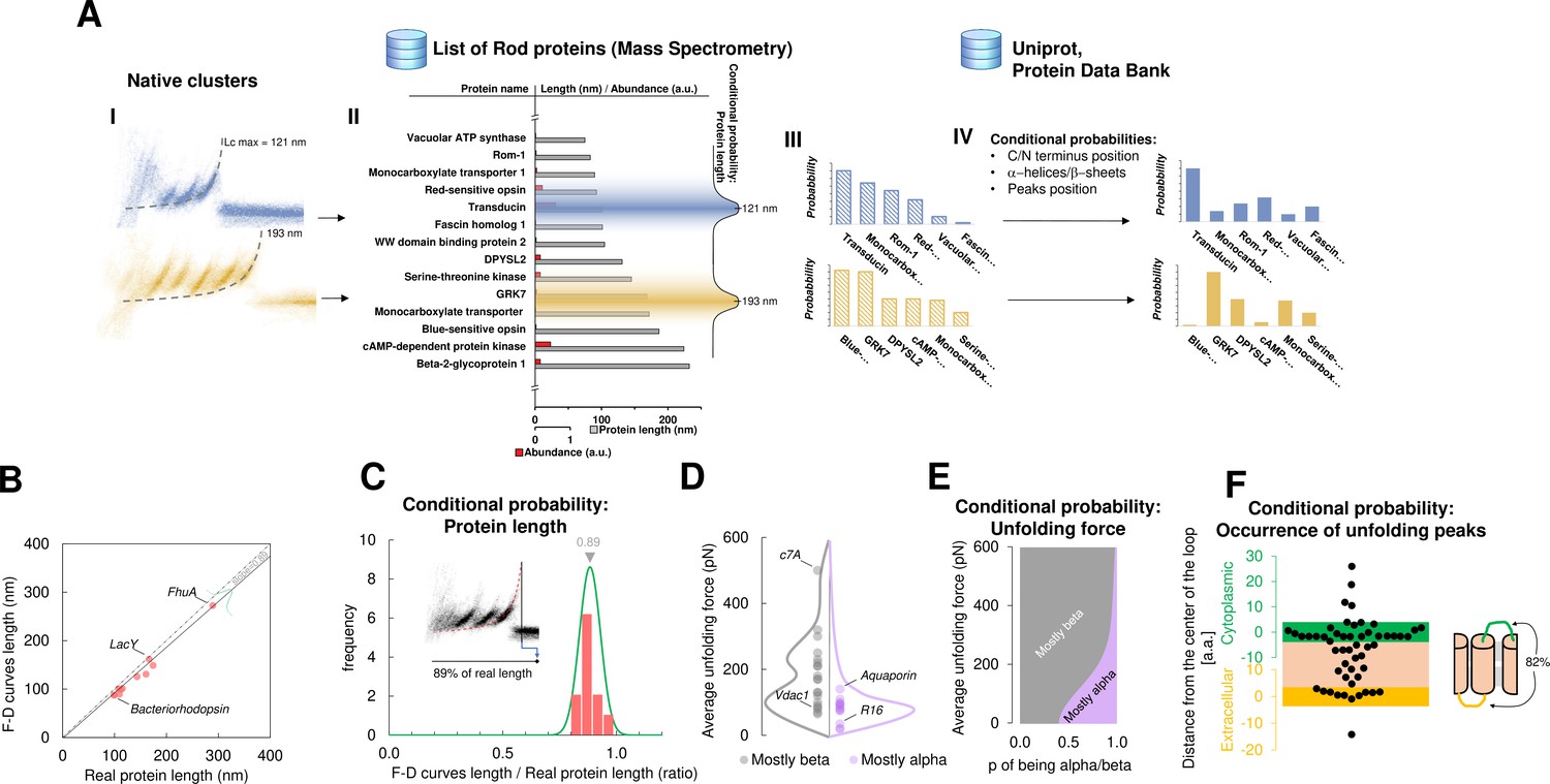
(A) Logical workflow of the Bayesian steps: selection due to total length and abundance (mass spectrometry), refinement with structural and topological information (PDB and Uniprot). (B) Comparison of the real length of the protein vs. the measured maximal contour length of the force-distance (F-D) curves in 14 single-molecule force spectroscopy (SMFS) experiments on membrane proteins (Pearson coefficient r=0.991). (C) Conditional probability of the observed maximal length of the clusters obtained from (B). (D) Comparison of the force necessary to unfold β-sheets and α-helices in 22 SMFS experiments. (E) Conditional probability of the observed unfolding forces obtained from (D). (F) Conditional probability for the occurrence of unfolding peaks extracted from SMFS literature (see Methods). Unfolding peaks occurs most likely in the loops (82%) than in transmembrane domains (n_peaks = 54, from 11 SMFS experiments of different membrane proteins). The points in the green (yellow) region represents unfolding peaks occurred in a cytoplasmic (extracellular) loop, the point in the pink area occurred in a transmembrane domain. The points above the green and below the yellow regions occurred in cytoplasmic and extracellular domains, respectively. The scale is approximate because in rare occasion loops are longer than 10 nm.
Figure 4—figure supplement 1

The cross-correlation used to evaluate .
(A) Global histogram of cluster NG8 and the density plot. (B) The peaks in (A) represent the region where the peaks tend to occur. (C) Ideal profile of TMEM16F built starting from the information that 86% of the peaks happen in the loops (D). (E) Superimposition of the real and the idealized profile: the correlation between the two generates a number that is used in the probability estimation. The more peaks correspond to loops, the higher is the cross-correlation value. (F) Blue dots indicate the location of force peaks in the cryo electron microscopy (cryo-EM) structure of the TMEM16F.
Figure 5
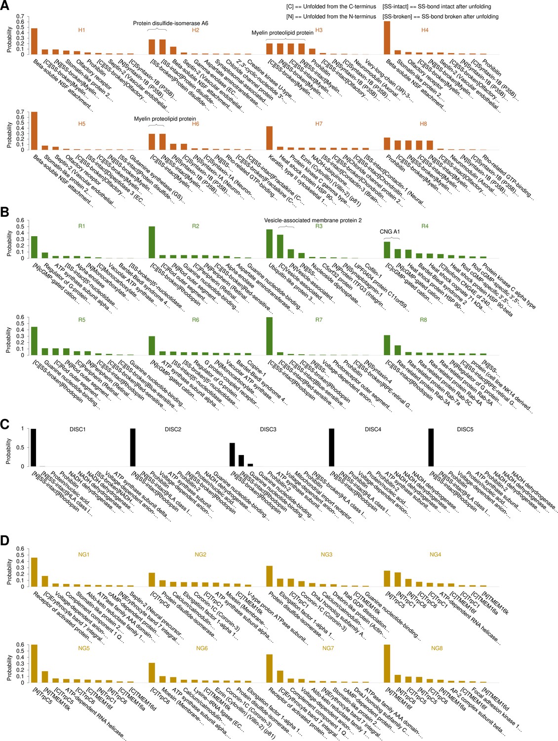
Bayesian identification of the unfolding clusters.
Most probable candidates for the unfolding clusters found in (A) hippocampal neurons; (B) rods; (C) rod discs; (D) NG108-15 cells.
Figure 6 with 1 supplement
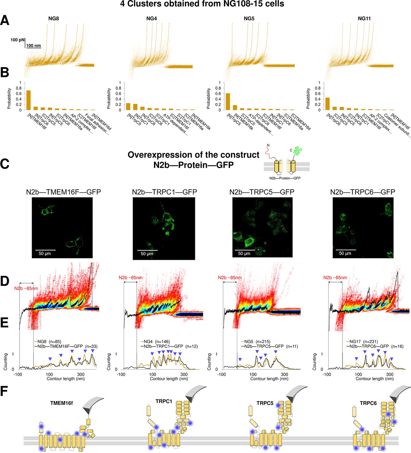
Validation of the method with a comparison between native clusters and those obtained with overexpression of a construct with the N2B signature at the N-terminal and GFP at the C-terminal.
(A) Four clusters found in the dataset of force-distance (F-D) traces pulled from NG108-15 cells wild type. (B) The Bayesian identification of the clusters in (A) with the candidate membrane proteins. (C) Confocal images of NG108-15 cells overexpressing the construct N2b-Protein-GFP, as reported by the green fluorescence emitted by GFP. (D) From left to right, color density plots (blue indicating a colocalization among F-D traces of more than 80%) of the clusters superimposed to an F-D curve bearing the N2B signature (85 nm segment with a flat force below 10 pN) obtained in the sample overexpressing the candidate protein TMEM16F, TRPC1, TRPC5, and TRPC6, respectively. (E) Global histogram of Lc of the clusters in A and the clusters with the N2B signature from cells transfected with the corresponding construct. (F) Position of the most likely rupture regions of the proteins according to (E) superimposed to the cartoon of the cryo electron microscopy (cryo-EM) structure available in the PDB.
Figure 6—figure supplement 1

Western blots for the four proteins indicating the silencing obtained with different plasmids.
(A–D) Control for the presence of TRPC1, TRPC5, TRPC6, tMEM16F. (E–H) Raw images of the gels with the marker bands.
-
Figure 6—figure supplement 1—source data 1
Photos of the western blots.
- https://cdn.elifesciences.org/articles/77427/elife-77427-fig6-figsupp1-data1-v2.zip
Figure 7 with 1 supplement
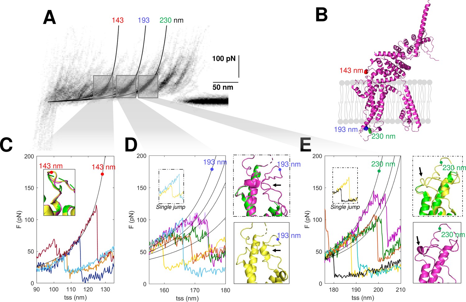
Structural segmentation in the loops of TRPC6.
(A) Density plot of force-distance (F-D) curves of TRPC6 (validated from cluster NG11). (B) 3D structure of TRPC6 (PDB: 6UZA) with highlighted the position corresponding to the unfolding peaks in (A). (C) Representative F-D curves showing the single peak at 143 nm. Insert: comparison of the agreement with the three proposed structures of TRPC6 (PDB ID, green: 5YX9; purple: 6UZA; yellow: 6UZ8). (D) Representative F-D curves showing the variable behavior at 193 nm where ~20% of the F-D curves shows a single jump that suggests no structural fragmentation of the loop like in the green/purple structures. Right inserts: comparison of the structure of the loop obtained by cryo electron microscopy (cryo-EM) where only the yellow structure shows the presence of a 2-turn helix. (E) Representative F-D curves at 230 nm where ~30% of the F-D curves shows a single jump that suggests no structural fragmentation of the loop like in the green/yellow structures. Right inserts: comparison of the structure of the loop obtained by cryo-EM where only the purple structure shows the presence of a 1-turn helix.
Figure 7—figure supplement 1
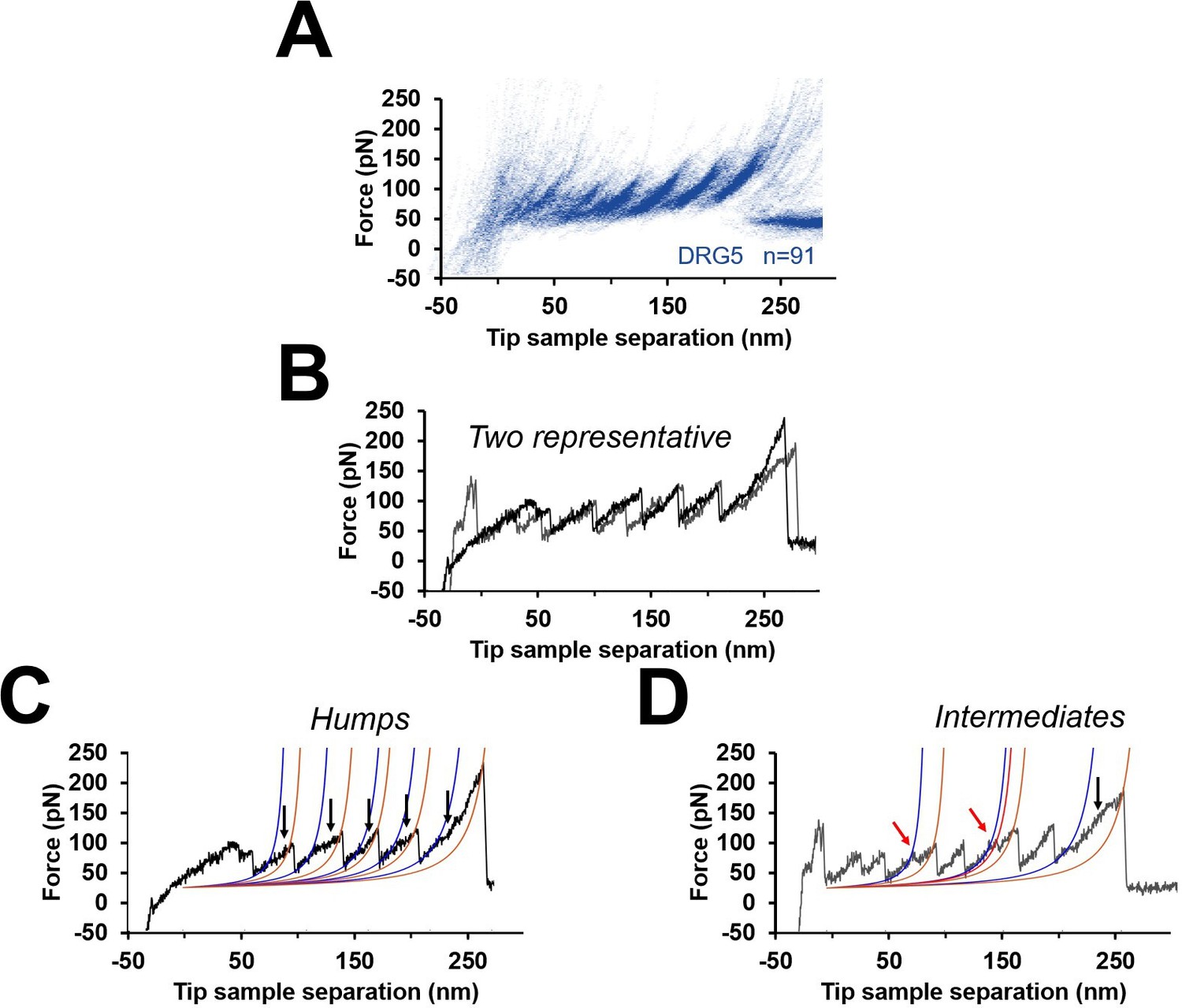
Unfolding intermediates and humps.
(A) Cluster DRG5 from Figure 3. (B) Two representative force-distance (F-D) curves from DRG5 (black and gray). (C) Black curve in (B) that shows humps (blue worm-like chain [WLC] fit identify the beginning of the humps, gold WLC fit identify the end). (D) Gray curve in (B) that shows multiple peaks (red arrows) instead of humps.
Tables
Key resources table
| Reagent type (species) or resource | Designation | Source or reference | Identifiers | Additional information |
|---|---|---|---|---|
| Gene (Mus musculus) | TMEM16F | PMID:34445284 | N/A | |
| Gene (Mus musculus) | TMEM16A | PMID:34089532 | N/A | |
| Gene (Spirochaeta thermophila) | SthK | PMID:30266906 | N/A | pCGFP-BC vector (modified by deleting the GFP and four out of the eight histidines) |
| Gene (Mus musculus) | Mouse TRPC1 | MiaoLing Plasmid Company (NM_011643.4) | N/A | |
| Gene (Mus musculus) | Mouse TRPC5 | MiaoLing Plasmid Company (NM_009428.3) | N/A | |
| Gene (Mus musculus) | Mouse TRPC6 | MiaoLing Plasmid Company (NM_013838.2) | N/A | |
| Gene (Mus musculus) | N2B | PMID:25963832 | N/A | |
| Strain, strain background (Escherichia coli) | DH5α | Thermo Fisher Scientific | Cat#18258012 | Competent cells |
| Strain, strain Background (Escherichia coli) | Stbl3 | Thermo Fisher Scientific | Cat#C7373-03 | Competent cells |
| Cell line (Mouse × Rat Hybrid) | NG108-15 cells | Sigma-Aldrich (China) | Cat#88112302 | |
| Transfected construct (Mus musculus) | TMEM16A-GFP | PMID:34089532 | N/A | peGFP-N1 backbone |
| Transfected construct (Mus musculus) | TMEM16F-GFP | PMID:34445284 | N/A | peGFP-N1 backbone |
| Transfected construct (Mus musculus) | 6xHis-N2B- mTMEM16F-GFP | GENEWIZ (China) | N/A | peGFP-N1 backbone |
| Transfected construct (Mus musculus) | 6xHis-N2B- mTRPC1-GFP | GENEWIZ (China) | N/A | peGFP-N1 backbone |
| Transfected construct (Mus musculus) | 6xHis-N2B- mTRPC5-GFP | GENEWIZ (China) | N/A | peGFP-N1 backbone |
| Transfected construct (Mus musculus) | 6xHis-N2B- mTRPC6-GFP | GENEWIZ (China) | N/A | peGFP-N1 backbone |
| Transfected construct (Mus musculus) | plentiCRISPR V2-TRPC1- sgRNA1 | MiaoLing Plasmid Company | N/A | sgRNA sequence ccgtaagcccacctgtaaga |
| Transfected construct (Mus musculus) | plentiCRISPR V2-TRPC1- sgRNA2 | MiaoLing Plasmid Company | N/A | sgRNA sequence acgcttgtagcagaagggct |
| Transfected construct (Mus musculus) | plentiCRISPR V2-TRPC5- sgRNA1 | MiaoLing Plasmid Company | N/A | sgRNA sequence attactctacgccatccgca |
| Transfected construct (Mus musculus) | plentiCRISPR V2-TRPC5- sgRNA2 | MiaoLing Plasmid Company | N/A | sgRNA sequence ggagtgtgtatccagttcgg |
| Transfected construct (Mus musculus) | plentiCRISPR V2-TRPC6- sgRNA1 | MiaoLing Plasmid Company | N/A | sgRNA sequence gcggcagacgattcttcgtg |
| Transfected construct (Mus musculus) | plentiCRISPR V2-TRPC6- sgRNA2 | MiaoLing Plasmid Company | N/A | sgRNA sequence taaaggttatgtacggattg |
| Transfected construct (Mus musculus) | plentiCRISPR V2-TMEM16F- sgRNA1 | MiaoLing Plasmid Company | N/A | sgRNA sequence agcgagcgttacctcctgta |
| Transfected construct (Mus musculus) | plentiCRISPR V2-TMEM16F- sgRNA2 | MiaoLing Plasmid Company | N/A | sgRNA sequence ctctcgggtcaaataccaag |
| Transfected construct (Mus musculus) | plentiCRISPR V2-control-sgRNA | MiaoLing Plasmid Company | N/A | sgRNA sequence tcttgagtttgtaacagctg |
| Transfected construct (Mus musculus) | mCherry-Lifeact-7 | Addgene | Plasmid #54491 | Actin labeled with mCherry |
| Biological sample (Rat) | Hippocampal and DRG neurons | Home-made | N/A | Freshly isolated from Wistar rats |
| Biological sample (Xenopus laevis) | Rod cells | Home-made | N/A | Freshly isolated from male Xenopus laevis |
| Antibody | Anti-TMEM16F (Rabbit polyclonal) | Alomone Labs | Cat#ACL-016 | WB(1:200) |
| Antibody | Anti-TRPC1 (Rabbit polyclonal) | Alomone Labs | Cat#ACC-010 | WB(1:500) |
| Antibody | Anti-TRPC5 (Rabbit polyclonal) | Alomone Labs | Cat#ACC-020 | WB(1:500) |
| Antibody | Anti-TRPC6 (Rabbit polyclonal) | Alomone Labs | Cat#ACC-120 | WB(1:500) |
| Antibody | Anti-α-Tubulin (Mouse monoclonal) | Sigma | Cat#T8203 | WB(1:5000) |
| Antibody | Goat Anti-Rabbit HRP (Goat polyclonal) | Dako | Cat#P0448 | WB(1:5000) |
| Antibody | Goat Anti-Mouse HRP (Goat polyclonal) | Dako | Cat#P0447 | WB(1:5000) |
| Peptide, recombinant protein | SthK | Home-made | N/A | |
| Peptide, recombinant protein | Hs Bacteriorhodopsin (bR) | Cube-Biotech | Cat#28903 | |
| Peptide, recombinant protein | Channelrhodopsin 1_Ca (ChR1) | Cube-Biotech | Cat#28941 | |
| Chemical compound, drug | TCEP | Sigma | Cat#C4706 | |
| Software, algorithm | Matlab2017a | MathWorks | N/A | |
| Software, algorithm | ImageJ 1.47v | NIH | RRID:SCR_003070 | |
| Other | Hoechst | Life Technologies | Cat#33342 | Stain the DNA in live cells without the need of permeabilization |
Additional files
-
Supplementary file 1
Tables with list of plasmids and sgRNA sequences.
- https://cdn.elifesciences.org/articles/77427/elife-77427-supp1-v2.docx
-
Supplementary file 2
Sample statistics (experiments and clusters).
- https://cdn.elifesciences.org/articles/77427/elife-77427-supp2-v2.docx
-
Supplementary file 3
Tables with proteins find with mass spectrometry.
- https://cdn.elifesciences.org/articles/77427/elife-77427-supp3-v2.zip
-
Transparent reporting form
- https://cdn.elifesciences.org/articles/77427/elife-77427-transrepform1-v2.pdf
Download links
A two-part list of links to download the article, or parts of the article, in various formats.
Downloads (link to download the article as PDF)
Open citations (links to open the citations from this article in various online reference manager services)
Cite this article (links to download the citations from this article in formats compatible with various reference manager tools)
Unfolding and identification of membrane proteins in situ
eLife 11:e77427.
https://doi.org/10.7554/eLife.77427


