Species clustering, climate effects, and introduced species in 5 million city trees across 63 US cities
- Department of Organismic and Evolutionary Biology, Harvard University, United States
- Department of Materials Science and Engineering, Stanford University, United States
- Hopkins Marine Station, Stanford University, United States
- Department of Biology, Duke University, United States
- Harvard Forest, Harvard University, United States
- Independent Researcher, United States
- Department of Biology and Biotechnology, Worcester Polytechnic Institute, United States
- The Biota of North America Program (BONAP), United States
Figures
Figure 1
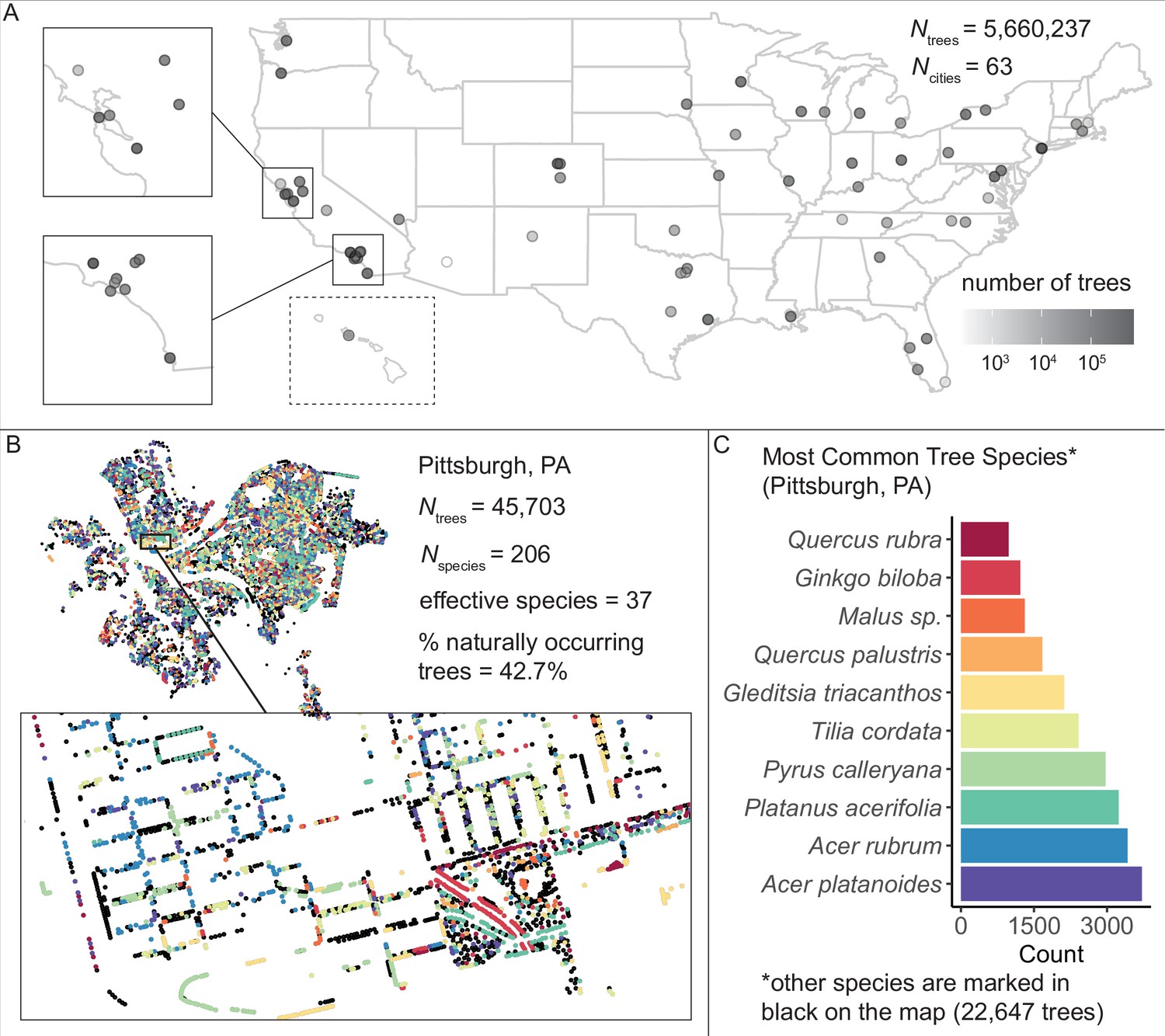
We assembled and standardized a dataset of N = 5,660,237 street trees from publicly available street tree inventories across 63 cities in the USA.
(A) The number of trees recorded per city varied from 214 (Phoenix, AZ) to 720,140 (Los Angeles, CA) with a median of 45,148. (B) Sample plot of Pittsburgh, PA with trees colored by species type (inset: zoomed-in view of trees lining streets and parks). We include statistics for total number of trees Ntrees = 45,703; total number of species Nspecies = 206; effective species count = 36 (a measure of diversity that incorporates both richness [number of species] and evenness [distribution of those species]; see Equation 1); and percent naturally occurring (rather than introduced) trees = 42.7%. (C) Counts of the 10 most common species inventoried in Pittsburgh; not shown are 22,647 trees belonging to other species (black points in (B)). The dataset includes information on species, exact location, whether a tree is introduced or naturally occurring, tree height, tree diameter, location type (green space or urban setting), tree health/condition, and more (Figure 1—source data 1). Source data are Figure 1—source data 1 and Figure 1—source data 2; source code is Source code 2.
-
Figure 1—source data 1
City_Trees_Data_63_Files.zip.
This zipped file includes all of the cleaned data used in the study (63 spreadsheets, one for each city, where each row is a tree). It is available on Dryad at https://doi.org/10.5061/dryad.2jm63xsrf.
- https://cdn.elifesciences.org/articles/77891/elife-77891-fig1-data1-v2.zip
-
Figure 1—source data 2
Tree_Data_Summary_By_City.csv.
Here, we present all results by city, including number of trees, percent native, effective species count, environmental variables, sociocultural variables, and more.
- https://cdn.elifesciences.org/articles/77891/elife-77891-fig1-data2-v2.csv
Figure 2 with 3 supplements
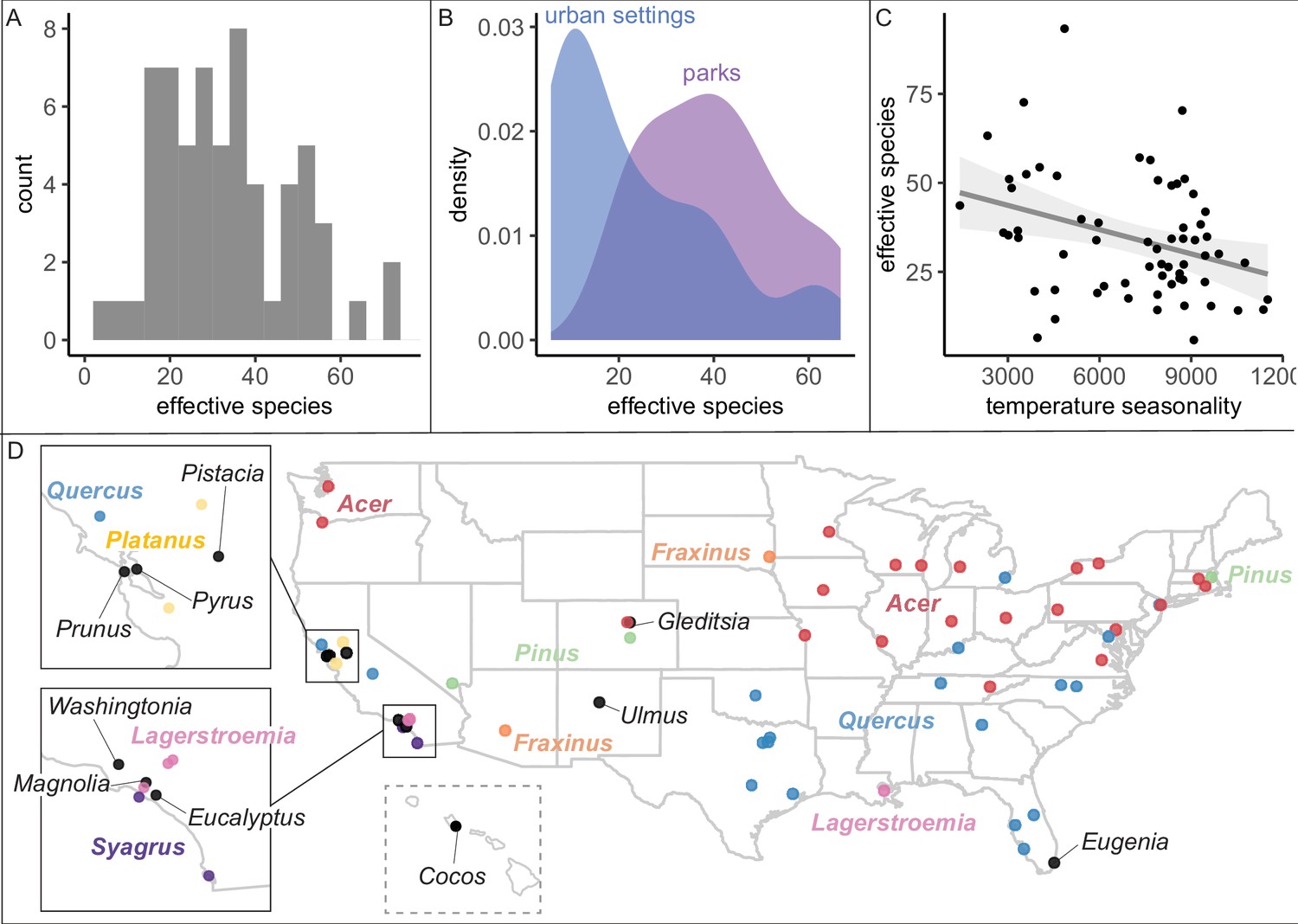
City tree communities are diverse and shaped by climate, although certain genera dominate.
(A) Effective species count, a measure of species diversity, ranged across cities from min = 6 to max = 93 with a median = 26. We use Shannon’s effective species count (Equation 1), a more nuanced metric than abundance-based metrics (see Figure 2—figure supplement 2). (B) Trees in parks were significantly more diverse than trees in urban settings such as along streets (two-sample paired t-test comparing effective species numbers; t = 7, p < 0.0005, 95% confidence interval [CI] = [11.8, 22.9], mean diff. = 17, degrees of freedom = 10.4). To account for differences in population size and sampling effort between areas, we calculated effective species number for a given population size (the smaller of the two options, park and urban, for each city) using rarefaction approaches in the R package iNext. Results were also significant for (1) raw effective species number and (2) asymptotic estimate of effective species number. See Figure 2—figure supplement 1 for sample sizes. (C) Environmental factors were significantly correlated with effective species count, across six sensitivity conditions controlling for sampling effort, population size, and more (Supplementary file 2). Most sociocultural variables were not significant, but cities designated as ‘Tree City USA’ were significantly more likely to have higher effective species numbers than those without that designation (for three of our six sensitivity analyses). Here, we plot the negative relationship between tree species diversity (effective species count controlling for population size) and temperature seasonality (captured through environmental PC1; see Supplementary file 5). To allow for comparison across cities with different sizes and sampling efforts, we plot the calculated effective species number for a population = 37,000 trees, the rounded median population size (using rarefaction and extrapolation in R package iNext). Results were also significant for (1) raw effective species number, (2) asymptotic estimate of effective species number, and when excluding cities with low sample size or sample coverage (Supplementary file 2). (D) The most abundant genus in each city is labeled here; see the most common species by city in Figure 2—figure supplement 3. Supporting figures for this figure include Figure 2—figure supplement 1, Figure 2—figure supplement 2, and Figure 2—figure supplement 3; Supplementary file 2 and Supplementary file 5 are supporting tables. Source data are Figure 1—source data 1, Figure 1—source data 2, and Figure 2—source data 1; source code is Source code 2; and an associated tool to calculate effective species is Source code 3.
-
Figure 2—source data 1
Rarefaction_Plots.zip.
This zipped file includes plots for the tree community of each city, showing rarefaction curves as calculated by the R package iNext. Each city includes a plot for all trees and a plot for all naturally occurring trees.
- https://cdn.elifesciences.org/articles/77891/elife-77891-fig2-data1-v2.zip
Figure 2—figure supplement 1
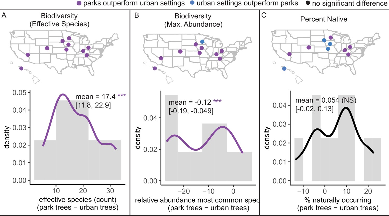
Tree communities in parks were significantly more biodiverse than those in urban settings but did not differ significantly in percent of trees that were naturally occurring (rather than introduced).
(A) Effective species numbers were greater in parks (two-sample paired t-test; t = 7.2, p < 0.0005, 95% confidence interval [CI] = [9.99, 18.6], mean diff. = 14.3, degrees of freedom = 10). For this calculation, we use the interpolated or extrapolated effective species number for a given population size (the smaller of the two populations being compared, park or urban). We found the same result for raw effective species number (t = 8.1, p = 1.1e−05, 95% CI = [13.2, 23.2], mean diff. = 18.2, degrees of freedom = 10) and for asymptotic estimate of effective species number (t = 5.1, p = 0.00045, 95% CI = [11.3, 28.9], mean diff. = 20.1, degrees of freedom = 10). (B) Maximum abundance of a single species was lower in parks (two-sample paired t-test; t = −3.7, p = 0.004, 95% CI = [−0.19, −0.049], mean diff. = −0.12, degrees of freedom = 10). (C) Percent naturally occurring did not differ significantly (two-sample paired t-test; t = 1.7, p = 0.13, 95% CI = [−0.019, 0.13], mean diff. = 0.054, degrees of freedom = 10). We confirmed normality of the differences using a Shapiro–Wilk normality test, and confirmed all results through non-parametric Wilcoxon ranked-sign tests. We had sufficient data from 11 cities: Aurora, CO, park trees N = 17,366, urban trees N = 32,455; Columbus, OH, park trees N = 22,791, urban trees N = 112,586; Denver, CO, park trees N = 252,695, urban trees N = 12547; Des Moines, IA, park trees N = 15,035, urban trees N = 174; Honolulu, HI, park trees N = 12,650, urban trees N = 974; Knoxville, TN, park trees N = 4821, urban trees N = 3551; Las Vegas, NV, park trees N = 23,636, urban trees N = 971; Louisville, KY, park trees N = 16,916, urban trees N = 4373; Minneapolis, MN, park trees N = 12,983, urban trees N = 175,232; Overland Park, KS, park trees N = 162, urban trees N = 38,898; and Sioux Falls, SD, park trees N = 12,672, urban trees N = 47,684. Note: the plot includes 11 cities, but Denver, CO and Aurora, CO appear as one dot at this zoomed-out level of resolution. Significance level *** indicates p<0.0005.
Figure 2—figure supplement 2
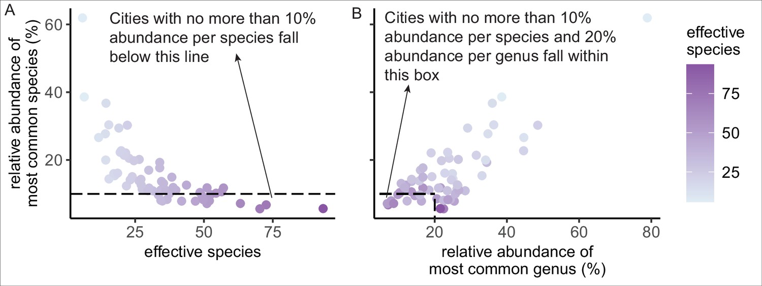
Effective species is a more nuanced metric of species diversity than the metric of the relative abundance of the most common species or genus.
(A) The simple metric of relative abundance of most common species correlated with the more nuanced metric of effective species count (Pearson’s product-moment correlation: cor = −0.63, 95% confidence interval [CI] = [−0.76, −0.46], t = −6.40, p < 0.0005). (B) Most cities did not fulfill Santamour’s 10/20 rule, as is evident in this plot of relative abundance of the most common species versus relative abundance of the most common genus.
Figure 2—figure supplement 3
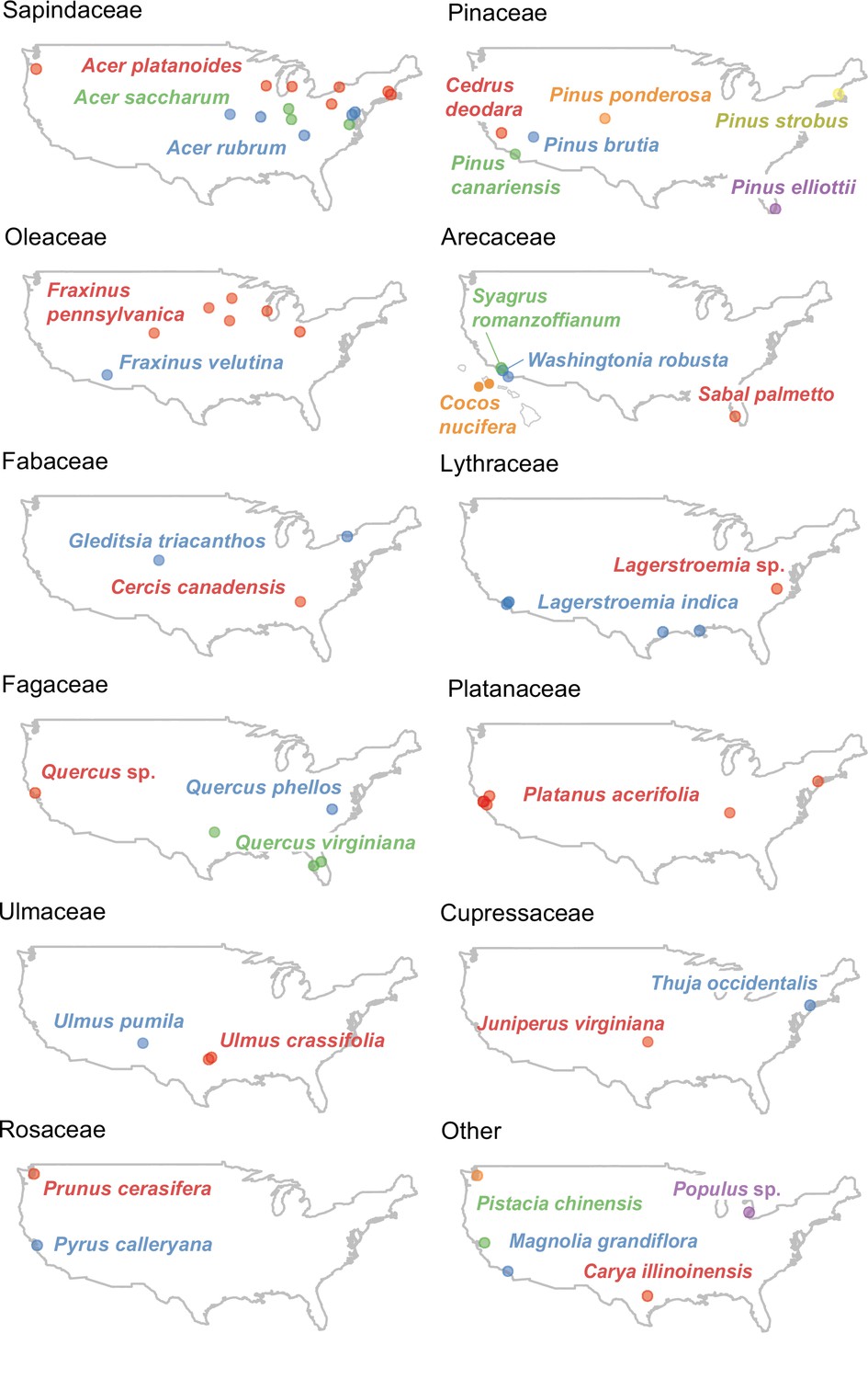
The most common tree species in each city is labeled.
The most common species in each city is labeled (organized by family for display purposes).
Figure 3 with 1 supplement
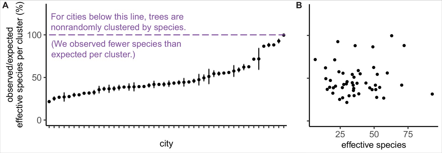
Trees are spatially clustered by species in nearly all cities, even in cities with high species diversity.
(A) In 47 of 48 cities, trees are non-randomly clustered by individual species (with significantly fewer effective species per spatial cluster than expected, i.e., values <100%). Plotted points represent median values and 95% confidence intervals (observed/expected effective species counts) for all clusters in a city (see Nclusters per city and full statistics in Figure 3—source data 1). We excluded one city, Greensboro, from the analysis due to insufficient sample size (10 clusters). (B) The degree of spatial clustering in a city was not correlated with effective species number, a measure of tree diversity (Figure 3—figure supplement 1). To control for different sizes and sampling efforts across cities, here we plot the calculated effective species number for a given population = 37,000 trees (using rarefaction and extrapolation in R package iNext). Ncities = 48. Figure 3—figure supplement 1 is a supporting figure for this figure. Source data are Figure 1—source data 1 and Figure 3—source data 1; source code is Source code 2.
-
Figure 3—source data 1
Clustering_Results.csv.
This file includes all statistics on clustering by species, including number of clusters, median effective species count per cluster, min, max, interquartile range, and 95% confidence interval (see Figure 2).
- https://cdn.elifesciences.org/articles/77891/elife-77891-fig3-data1-v2.csv
Figure 3—figure supplement 1

The degree to which a city has trees clustered by species does not correlate with abundance-based measures of species diversity.
Clustering score is the observed/expected effective species per cluster (see ‘Materials and methods’ and Main Text). (A) Clustering score is not correlated with the relative abundance of the most common species. (B) Clustering score is not correlated with the relative abundance of most common genus.
Figure 4 with 1 supplement
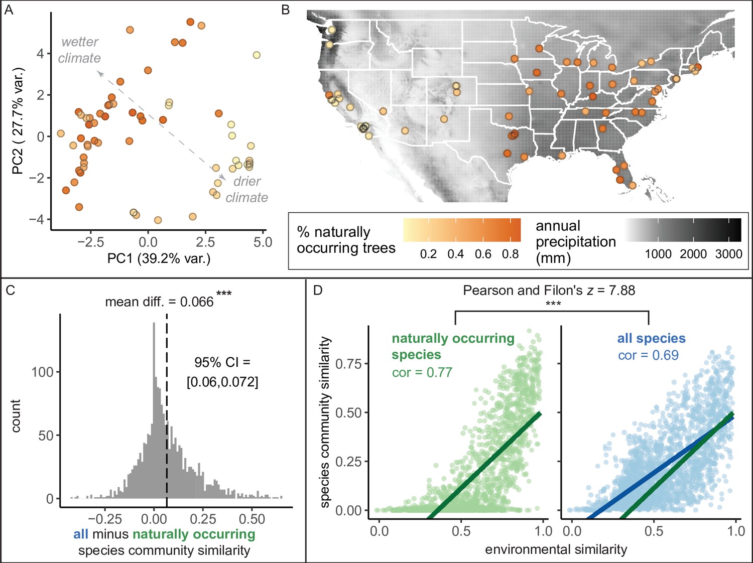
Environment strongly influences the percentage of naturally occurring trees, while introduced trees make species compositions more similar between cities.
(A) Cities in wetter, cooler climates—and younger cities—had significantly higher percentages of naturally occurring (rather than introduced) trees (beta regression; AIC = −58.4, pseudo-R2 = 0.64, log likelihood = 35.2; statistics in Supplementary file 3). Indeed, we found that wetter, cooler climates significantly predicted higher percentages of naturally occurring trees across four sensitivity tests: excluding outliers (Ncities = 61); including cities with >10,000 trees (Ncities = 49); including cities with >50% spatial coverage (Ncities = 28); and including cities with high sample coverage (Ncities = 56). See Supplementary file 3. Here, we plot a principal component analysis of the Bioclim variables (Figure 4—source data 2), colored by percent naturally occurring trees. Each point represents one city. Bioclim variables relating to precipitation (such as annual precipitation) are negatively correlated with PC1 and positively correlated with PC2 (see complete loadings in Supplementary file 5). (B) The percent of naturally occurring trees is plotted against annual precipitation in mm (black and white background). (C) Among city pairs (Ncomparisons = 1953), overall species communities are significantly more similar to one another than their naturally occurring species communities alone (paired t-test, t = 20.4, p < 0.0005, 95% confidence interval [CI] = [0.060, 0.072], mean difference = 0.066, degrees of freedom = 1,952; result upheld by non-parametric Wilcoxon signed-rank test). We calculated chi-square similarity scores for each pair of cities under two conditions; first, we included all trees (‘all’), then we included only naturally occurring trees (‘naturally occurring’), and reported the difference between the two similarity scores. We controlled for different population sizes and sampling efforts by randomly subsampling the larger city in the pairwise comparison 50 times and calculating the median chi-squared similarity score from those 50 repetitions. (D) Among city pairs, environment is significantly more strongly related to naturally occurring species than introduced species. We compared chi-square similarity scores between species communities (left: naturally occurring only; right: all) against environmental similarity scores (one minus the normalized euclidean distance in our principal components analysis [PCA]). Left panel, green, naturally occurring species only: Pearson’s product-moment correlation, cor = 0.77, 95% CI = [ 0.75, 0.78], t = 52.7, p < 0.0005, degrees of freedom = 1,952. Right panel, blue, all species: Pearson’s product-moment correlation; cor = 0.69, 95% CI = [0.67, 0.71], t = 42.0, p < 0.0005, degrees of freedom = 1,952. In the right panel, the green line is the same as in the left panel to enable comparisons. Figure 4—figure supplement 1 is a supporting figure for this figure, and Supplementary file 3 and Supplementary file 5 are supporting tables for this figure. Source data are Figure 1—source data 1, Figure 1—source data 2, Figure 4—source data 1, Figure 4—source data 2, and Figure 4—source data 3; source code is Source code 2; and an associated tool to label each species in a list of treespecies as ‘naturally occurring’ or ‘introduced’ is Source code 4. Significance level *** indicates p<0.0005.
-
Figure 4—source data 1
Native_Taxa_By_State_BONAP.csv.
This csv file includes a list of all naturally occurring (i.e., “native”) taxa observed in each US state, from the Biota of North America Project.
- https://cdn.elifesciences.org/articles/77891/elife-77891-fig4-data1-v2.csv
-
Figure 4—source data 2
Environmental_PCA.xlsx.
This file includes all loadings and scores for the environmental principal components analysis (PCA) (see Figure 3A).
- https://cdn.elifesciences.org/articles/77891/elife-77891-fig4-data2-v2.xlsx
-
Figure 4—source data 3
Spatial_Coverage_Analysis.zip.
This zipped file includes the plots showing the spatial distribution of all trees in a city for each city, as well as two CSV files with statistics about each city in raw form and summary form.
- https://cdn.elifesciences.org/articles/77891/elife-77891-fig4-data3-v2.zip
Figure 4—figure supplement 1
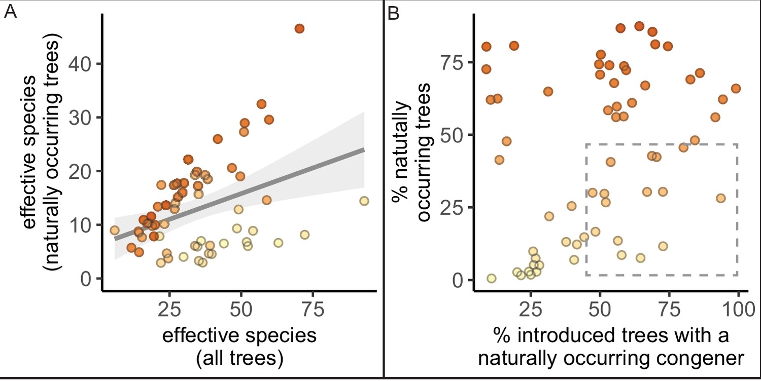
The percent of trees that are naturally occurring rather than introduced is not the only important variable when considering nativity status; here, we plot the species diversity of naturally occurring trees and percent of introduced trees that are closely related to naturally occurring trees (have a naturally occurring congener).
(A) The diversity of all naturally occurring trees (y-axis) is significantly correlated with the diversity of all trees (Pearson’s product-moment correlation; cor = 0.35, 95% confidence interval [CI] = [0.11, 0.55], p = 0.0052). To allow for comparison across cities with different sizes and sampling efforts, we plot the calculated effective species number for the rounded median population of all trees (for all species, 37,000 trees; x-axis) and native species only (10,000 trees; y-axis)—calculated using rarefaction and extrapolation in R package iNext. (B) The percent of all trees in a city that are naturally occurring is not significantly related to the percent of all introduced trees that have a naturally occurring congener. Cities with a low proportion of naturally occurring trees (but high proportion of introduced trees with a naturally occurring congener) are indicated with the gray dashed box.
Figure 5
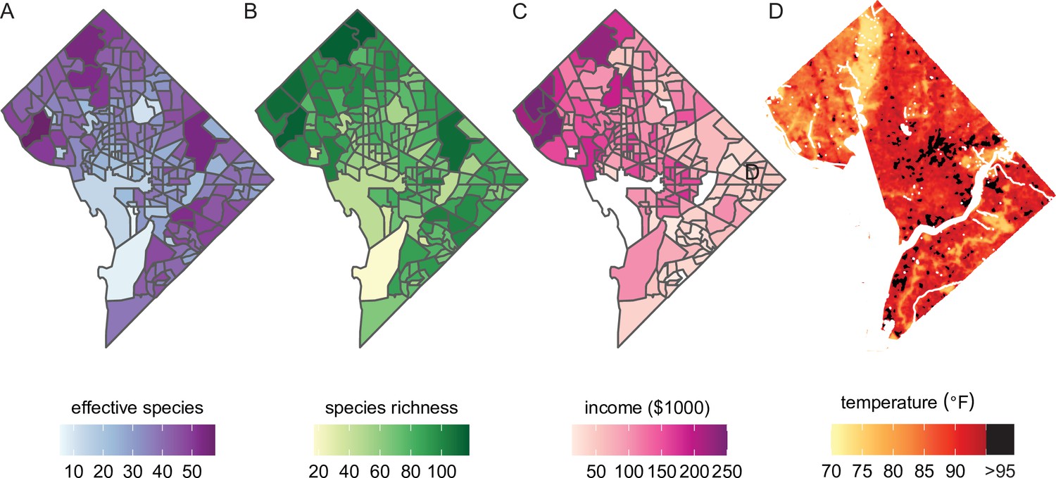
Future analyses could combine this city trees data with social, demographic, or physical variables (including income and urban heat islands).
Here, we plot different variables for Washington, DC, showing qualitative concordance between (A, B) measures of species diversity, (C) household income, and (D) the location of urban heat islands. (A) Effective species count is highest in the northwest and varies by census tract from 7 species to 54 species (median = 35 species). (B) Species richness is also highest in the northwest and varies by census tract from 17 species to 118 species (median 77 species). (C) Median household income is highest in the northwest, the region which overlaps substantially with the most biodiverse city tree communities. (D) Land surface temperatures in July 2018 are plotted to show the spatial location of the highest temperatures, including urban heat islands with temperatures >95°F. Source data are Figure 1—source data 1 and open-access data available from the US Census and the DC Open Data Portal (see ‘Materials and methods’) and source code is Source code 2.
Scheme 1

Dataset search pipeline.
Author response image 1

Author response image 2
Author response image 3
Additional files
-
Supplementary file 1
Here, we define the standardized columns used herein.
- https://cdn.elifesciences.org/articles/77891/elife-77891-supp1-v2.xlsx
-
Supplementary file 2
Here, we report the results of linear regression models analyzing diversity of the tree communities.
We ran six sensitivity analyses as follows. In Model 1, the independent variable was effective species as calculated for a given population of 37,000 trees (‘effective species for a standardized population size’). In Model 2, the independent variable was the asymptotic estimate of the effective species number for that city as calculated using iNext. In Model 3, the independent variable was the raw effective species number. In Model 4, we excluded cities with fewer than 10,000 trees. In Model 5, we excluded cities with <50% spatial coverage. In Model 6, we excluded cities with <0.995 sample coverage as calculated by iNext. For Models 4—6, the independent variable was effective species for a standardized population size of 37,000 trees. We use p = 0.05 as our threshold for significance; it is important to note that we do not apply a Bonferroni multiple-testing correction, because these are sensitivity analyses repeating the original test (rather than new, but statistically related, hypothesis tests).
- https://cdn.elifesciences.org/articles/77891/elife-77891-supp2-v2.xlsx
-
Supplementary file 3
Here, we report the results of beta regression models with independent variable percent naturally occurring trees (percent of trees that occur naturally in that region rather than being introduced).
We ran five models as sensitivity analyses to check for effects of population size, sample completeness, and spatial coverage, In Model 1, we include all cities. In Model 2, we excluded the outlier cities Honolulu, HI and Miami, FL. In Model 3, we excluded cities with fewer than 10,000 trees. In Model 4, we excluded cities with <50% spatial coverage. In Model 5, we excluded cities with <0.995 sample coverage as calculated by iNext. We use p = 0.05 as our threshold for significance; it is important to note that we do not apply a Bonferroni multiple-testing correction, because these are sensitivity analyses repeating the original test (rather than new, but statistically related, hypothesis tests).
- https://cdn.elifesciences.org/articles/77891/elife-77891-supp3-v2.xlsx
-
Supplementary file 4
We ran logistic regression models to identify correlations between condition and (1) tree size, (2) tree location, and (3) whether a tree was naturally occurring or introduced.
For size, smaller trees (lower diameter at breast height) tended to have better condition (12 of 18 cities). For location type, trees in the built environment tended to have better condition than those in parks (four of eight cities). For native status, results were mixed (naturally occurring trees had no difference in condition for 6 of 19 cities, worse condition in 7 cities, and better condition in 6 cities). Significant odds ratios and models are marked with *p < 0.05, **p < 0.005, ***p < 0.0005, or NS: p ≥ 0.05.
- https://cdn.elifesciences.org/articles/77891/elife-77891-supp4-v2.xlsx
-
Supplementary file 5
Loadings for the environmental principal component analysis in Figure 4A.
The Bioclim variables having to do with precipitation are negatively correlated with PCA1 and positively correlated with PCA2. When PCA1 is high and PCA2 is low, precipitation is higher. Likewise, when PCA1 is low and PCA2 is high, precipitation is lower. For example, refer to loadings for Annual_Precip and Precip_Driest_Month.
- https://cdn.elifesciences.org/articles/77891/elife-77891-supp5-v2.xlsx
-
Transparent reporting form
- https://cdn.elifesciences.org/articles/77891/elife-77891-transrepform1-v2.docx
-
Source code 1
Code_for_Data_Cleaning.zip.
This zipped file includes all code sheets in Python and R, and instructions, for the full data cleaning procedure (see ‘Materials and methods’, Data Cleaning).
- https://cdn.elifesciences.org/articles/77891/elife-77891-code1-v2.zip
-
Source code 2
Code_for_Analysis_and_Plotting.zip.
This zipped file includes all code used to analyze and plot the results reported in this paper.
- https://cdn.elifesciences.org/articles/77891/elife-77891-code2-v2.zip
-
Source code 3
Calculate_Effective_Species_Excel_Tool.xlsx.
We developed an Excel Spreadsheet which calculates effective species counts, a robust measure of species diversity, from a list of all trees (each row is an individual tree).
- https://cdn.elifesciences.org/articles/77891/elife-77891-code3-v2.zip
-
Source code 4
Check_Native_Status_of_Species_Excel_Tool.xlsx.
This Excel Workbook allows readers to input their list of species, select a state, and receive a corresponding list of whether or not each species is native to that state (based on BONAP designations).
- https://cdn.elifesciences.org/articles/77891/elife-77891-code4-v2.zip
Download links
A two-part list of links to download the article, or parts of the article, in various formats.
Downloads (link to download the article as PDF)
Open citations (links to open the citations from this article in various online reference manager services)
Cite this article (links to download the citations from this article in formats compatible with various reference manager tools)
Species clustering, climate effects, and introduced species in 5 million city trees across 63 US cities
eLife 11:e77891.
https://doi.org/10.7554/eLife.77891


