Figures and data in Vein fate determined by flow-based but time-delayed integration of network architecture

Figures
Videos
Tables
Additional files

20 figures, 11 videos, 4 tables and 1 additional file

Figures

Figure 1

Download asset Open asset

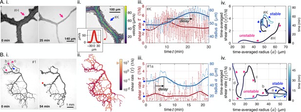
Diverse vein dynamics emerge during network reorganization.

(A) Close-up and (B) full network analysis of vein radius dynamics and associated shear rate in *P. polycephalum*. (i) Bright-field images of reorganizing specimens allow us to record vein dynamics. (ii) Velocity measurements: (A) Velocity profiles along vein segments extracted with particle image velocimetry (inset: profile along vein cross-section) and (B) vein contractions driving internal flows over the entire network are integrated to calculate shear rate in veins (here shown at the initial observation time). The color scale indicates the magnitude of shear rate in each colored vein segment. For example, the yellow arrow points to a vein with a high calculated shear rate. (**iii**) Change in shear rate preceding changes in vein radius, both shown as a function of time (connected dots) and their time-averaged trends (full lines). (**A.iii**) shows the dynamics in the vein #K from (**A.ii**), (**B.iii**) shows the vein marked in blue in (**B.i**). (iv) The time-averaged shear rate versus the time-averaged radius displays circling dynamics for stable veins and diverse qualitative dynamics for unstable, vanishing veins. Blue color shades encode time. Trajectory arrow colors match arrow colors marking vein position in A.i (#H), A.ii (#K) and B.i, respectively. Veins marked in pink are shrinking, while stable veins are in blue.

Figure 2

Download asset Open asset

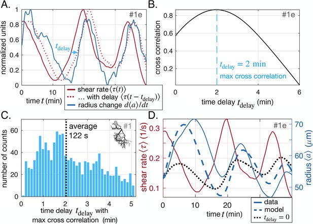
Shear rate induces vein adaptation with a time delay.

(A) Principle of the cross-correlation in time between the delayed time-averaged shear rate $⟨ τ (t - t_{delay}) ⟩$ and the time-averaged radius change $\frac{d ⟨ a ⟩}{d t} (t)$ . The plot shows the delayed curve with the best score. (B) Resulting cross-correlation for various values of $t_{d e l a y}$ and maximum extracted. (C) Statistical analysis over all veins of specimen #1 of maximal cross-correlation with $t_{d e l a y}$ , zoomed in on positive time delays, since they outnumber negative time delays by a factor of 15, see Appendix 2—figure 2 for full distribution. (D) Fit result of the model Equation 1 and Equation 2, here, with $t_{adapt} = 37 \pm 2 \min$ and $τ_{0} = 1.1 \pm 0.2 s^{- 1}$ (heavy dashed blue). The vein investigated is the same as in (**A–B**) and hence we took $t_{delay} = 2 \min$ . The relative fitting error is $ϵ_{err} = 0.07$ . The fit result of model Equation 1 taking $τ_{s} = ⟨ τ ⟩$ , *i.e*. with $t_{delay} = 0$ is also shown (heavy dotted black), and has error $ϵ_{err} = 0.11$ .

Figure 3

Download asset Open asset

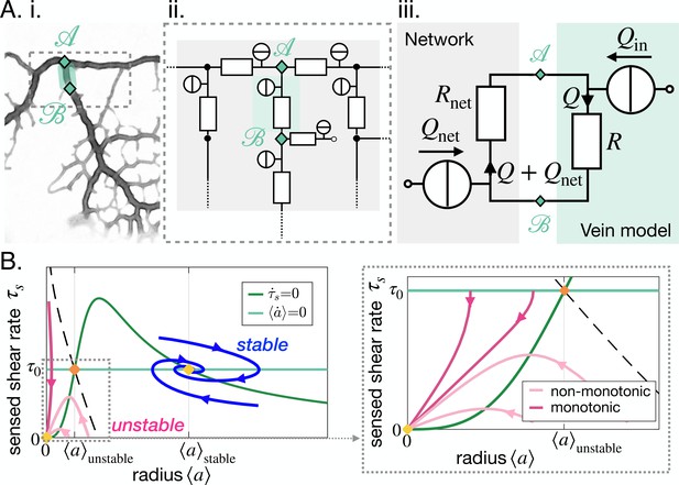
Stable and unstable vein dynamics are predicted within the same model.

(A) Translation of (i) a bright field image of specimen into (ii) vein networks; each vein is modeled as a flow circuit link. (iii) Reduction of (ii) via Northon’s theorem into an equivalent and simplified vein flow circuit consisting of a flow source $Q_{in}$ (due to vein’s pumping) and a resistor $R$ (viscous friction). The rest of the network is modeled by an equivalent circuit with flow source $Q_{net} = - Q_{in}$ and resistor $R_{n e t}$ . $Q$ flows through the vein. (B) (Left) Time-averaged sensed shear rate $τ_{s}$ versus radius from (1)-(3) with fixed points and typical trajectories. The green lines correspond to stationary solutions for $τ_{s}$ or $⟨ a ⟩$ . The blue lines correspond to stable trajectories and the pink lines to unstable ones. (Right) Zoom of the phase space corresponding to shrinking veins, including monotonic and non-monotonic trajectories.

Figure 4

Download asset Open asset

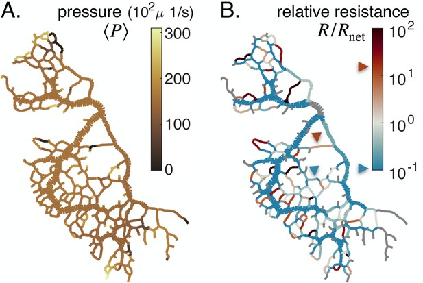
Feedback parameters integrate the network’s architecture and provide information on vein relative location.

Full network maps of the same specimen as in Figure 1B, at the beginning of the observation, of (A) the average fluid pressure in a vein $⟨ P ⟩$ and (B) of the relative resistance $R / R_{net}$ . The fluid pressure $⟨ P ⟩$ is defined up to an additive constant. Grey veins in (B) correspond to bottleneck veins or dangling ends for which $R_{net}$ can not be defined. The color scales indicate the magnitude of each variable in each colored vein. For example, in (B), the red arrow indicates a vein with large relative resistance $R / R_{net}$ .

Figure 5

Download asset Open asset

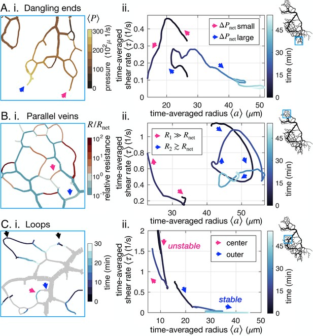
Network architecture controls vein fate as exemplified in three cases.

(**A–C**) (i) determining factors mapped out from experimental data for the specimen of Figure 1B and (ii) typical trajectories from data. All pink (respectively blue) arrows indicate shrinking (respectively stable or growing) veins. (A) (ii) Dangling ends either vanish or grow indefinitely, coherently with (i) the relative local pressure $⟨ P ⟩$ . Arrows point to veins initially similar in size (~23 μm). (B) Parallel veins are unstable: one vanishes in favor of the other one remaining (ii), coherently with (i) its relative resistance, $R / R_{net}$ , being higher. (C) Loops first shrink in the center of the loop (ii) – that is from the point furthest away from the nodes connecting it to the rest of the network – as evidenced by focusing on (i) the time of vein segment vanishing. Black arrows point to other loops also vanishing from the center. For all graphs on the left, the color scales indicate the magnitude of each variable in each colored vein.

Figure 6

Download asset Open asset

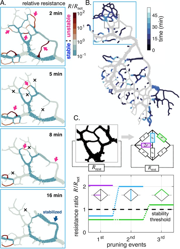
Avalanche of sequentially vanishing veins.

(A) Time series of network reorganization. Each vein is colored according to the ratio between the resistance of an individual vein $R$ and the rest of the network $R_{net}$ in each vein. Red arrows highlight vanishing veins in the experiment; black crosses indicate veins that disappeared within the previous time frame. Veins for which the relative resistance cannot be calculated, such as dangling ends, are plotted with $R / R_{net} = 1$ . (B) Map indicating vanishing vein events, with veins colored according to their disappearance time reported in the color scale. Gray veins will remain throughout the experiment. (C) Dynamics of the relative resistance of the three color-coded veins within a minimal network, inspired by the highlighted gray region of the network in (B). Vein resistances are chosen as $R = r$ except for a perturbed vein for which $R = 2 r$ . $R_{r e s t}$ represents the rest of the network relative to the region.In this model, a vein vanishes if its individual relative resistance $R / R_{n e t} > 1$ . The disappearance of veins sequentially increases the relative resistance of neighboring veins, making them unstable. Here $r / R_{rest} = 0.1$ , yet similar behavior was obtained consistently over a wide range of $r$ values.

Appendix 1—figure 1

Download asset Open asset

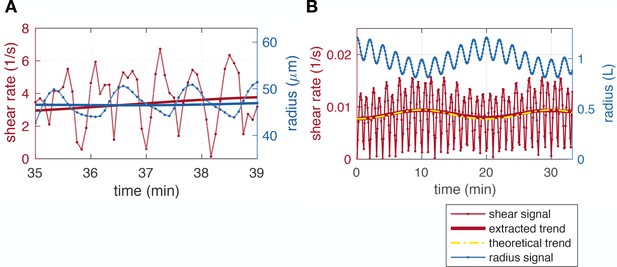
Extracting average shear rates from shear rate data.

(A) Time zoom of a close-up data set (that of Figure 1A.iii, #K) showing the doubling of the frequency of the shear rate compared to the radius. (B) Minimal model example with short timescale and long timescale radius oscillations, resulting in shear rate with a doubled frequency. Here, the contraction period $T = 2 \min$ and $t_{adapt} = 20 \min$ .

Appendix 1—figure 2

Download asset Open asset

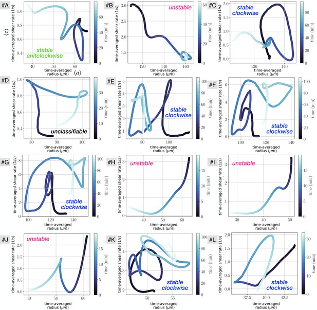
Vascular adaptation dynamics for all close up experiments, using time-averaged shear rates $⟨ τ ⟩$ and time-averaged radius $⟨ a ⟩$ .

The letters indicate the data set names, and are used consistently throughout the manuscript. Typical classification of vein dynamics is indicated for each plot.

Appendix 1—figure 3

Download asset Open asset

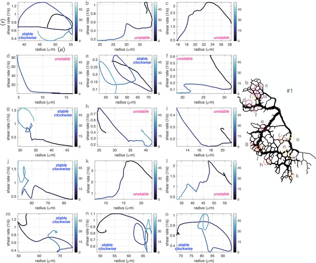
Vascular adaptation dynamics for a few veins in the full network #1 using time-averaged shear rates $⟨ τ ⟩$ and time-averaged radius $⟨ a ⟩$ .

The veins shown are chosen randomly but distributed throughout the network. The network sketch on the right hand side shows circles indicating at their center the location of each vein, with consistent labels. Typical classification of vein dynamics is indicated for each plot.

Appendix 1—figure 4

Download asset Open asset

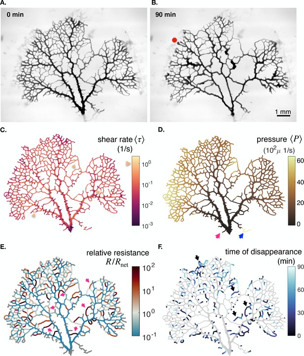
Additional data on the full network specimen #2.

(**A - B**) Bright field images of a specimen with long time dynamics of vanishing veins, specimen 2. (c) Mean shear rate $⟨ τ ⟩$ , (D) pressure $⟨ P ⟩$ and (E) relative resistance $R / R_{net}$ at the initial stage. (F) Time of vein disappearance for the entire experiment. See text for more information on the arrows and what to take out from the color maps.

Appendix 1—figure 5

Download asset Open asset

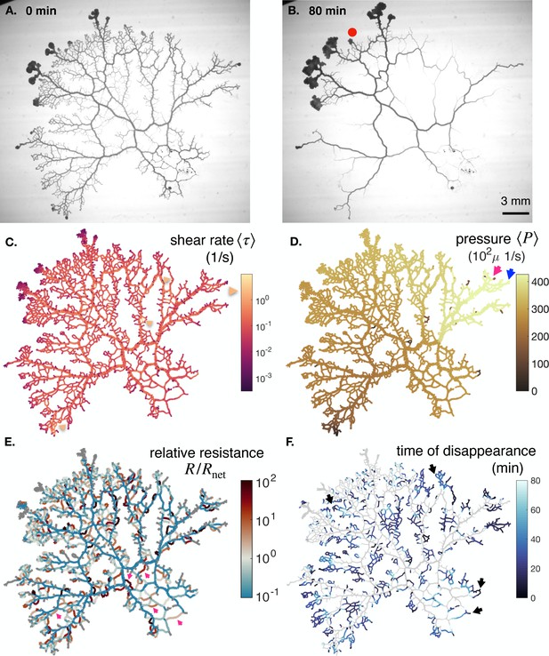
Additional data on the full network specimen #3.

(**A–B**) Bright field images of a specimen with long time dynamics of vanishing veins, specimen . (c) Mean shear rate $⟨ τ ⟩$ , (D) pressure $⟨ P ⟩$ and (E) relative resistance $R / R_{net}$ at the initial stage. (F) Time of vein disappearance for the entire experiment. See text for more information on the arrows and what to take out from the color maps.

Appendix 1—figure 6

Download asset Open asset

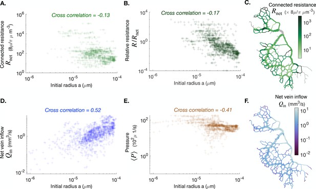
Cross correlation between average vein radius and different flow-based parameters (A) the connected resistance $R_{net}$ , (B) the relative resistance $R / R_{net}$ , (C) the vein outflow $Q$ and (E) the local pressure $⟨ P ⟩$ .

We also present maps of the connected resistance $R_{net}$ in (C) and of the vein outflow $Q$ in (F). The color scales indicate the magnitude of each variable in each colored vein. All cross-correlations and maps are done at the initial observation time for the full network specimen #1.

Appendix 2—figure 1

Download asset Open asset

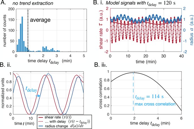
Time delay extracted is independent of averaging technique or oscillation frequency.

(A) Time delays measured without extracting trends from data (same plot as Figure 2C but without extracting trends). (B) Extracting the time delay for model data with (i) model data and extracted trends, (ii) extracted trends and best time delay obtained shown on trends and (iii) cross correlation between $d a / d t (t)$ and $τ (t - t_{delay})$ with respect to the searched time delay $t_{d e l a y}$ , and maximum value shown.

Appendix 2—figure 2

Download asset Open asset

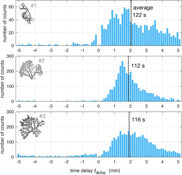
Time delay statistics from full networks.

Distribution of best time delays for all veins in the network (#1, with about 10,000 vein segments and #2 and #3, both of which have about 30,000 vein segments). (insets). Network maps – not to scale.

Appendix 2—figure 3

Download asset Open asset

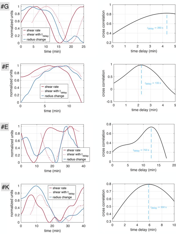
Time delays obtained with cross-correlation method on stable close-up data sets.

(Left hand side) Time-averaged shear rate $⟨ τ ⟩$ (red) and radius change ( $d ⟨ a ⟩ / d t$ ) with time for each vein (#E, #F, #G, #K), as well as time delayed shear right producing the best cross correlation $⟨ τ (t - t_{delay}) ⟩$ . (Right hand side) Cross-correlation with varying time delay and optimal time delay obtained at the correlation maximum.

Appendix 2—figure 4

Download asset Open asset

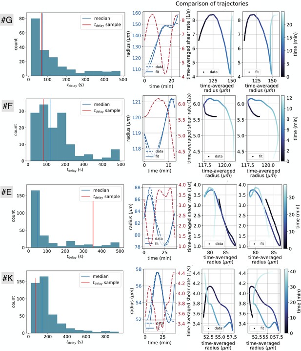
Evaluation of all three model parameters $t_{a d a p t}$ , $t_{d e l a y}$ and $τ_{0}$ from suitable data sets (#E, #F, #G, #K).

In the left column the distribution of the obtained time delays using Equation 1 and Equation 2 over a distribution of time windows is depicted. To obtain time windows of approximately constant model parameters we performed a fit for every possible time window with the constraints of a reasonable range of fitting parameters and time windows greater than 10 min. The right columns (three graphs) depict a sample of the results of a fitted trajectory, with a given time delay $t_{d e l a y}$ highlighted on the left hand side graphs as ‘ $t_{d e l a y}$ sample’. Among the three graphs on the right, the first, shows the fitted radius data as a function of time and the two next, show the data and the fitted result trajectories in the phase space with shear rate and radius.

Appendix 2—figure 5

Download asset Open asset

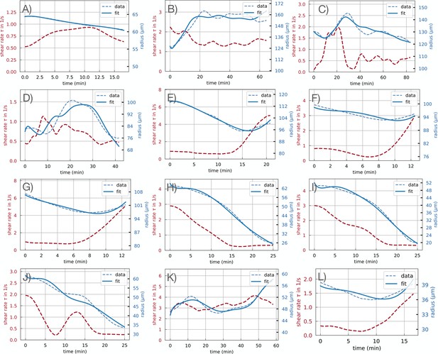
Fit results graphical representation of model Equation 1 and Equation 2 using a fixed time delay of $t_{d e l a y} = 120 s$ for all 12 close-up data sets on a given time window for each data set.

The obtained fit parameters are reported in Appendix 2—table 2. All shear rate and radius data presented is time-averaged.

Appendix 2—figure 6

Download asset Open asset

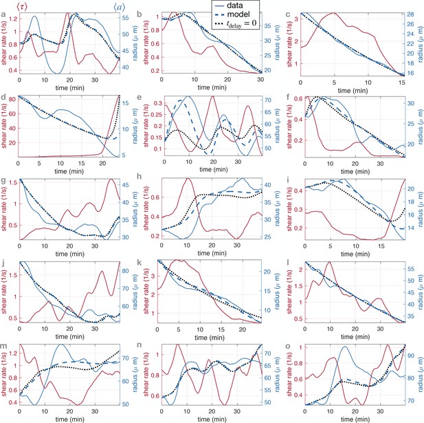
Fit results of model Equation 1 and Equation 2 for 15 randomly selected veins on specimen #1.

The corresponding fitted parameters are reported in Appendix 2—table 3. The vein positions correspond to those indicated in Appendix 1—figure 3.

Appendix 3—figure 1

Download asset Open asset

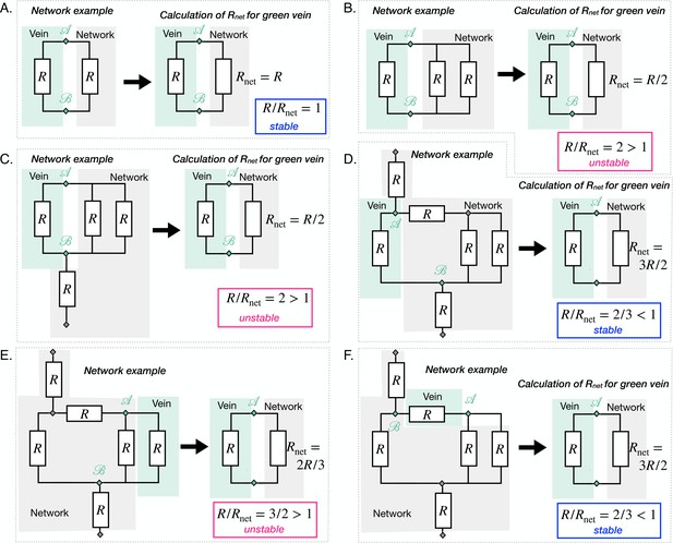
Principle of the calculation of $R_{net}$ on the basis of a few examples.

The networks are different in all cases except networks D-E-F are the same. D-E-F differ in which vein is under scrutiny. For each case, equivalent resistances $R_{net}$ of the rest of the network relative to the vein under scrutiny are calculated via Kirchhoff’s laws. The resulting $R_{net}$ is compared to $R$ . When $R > R_{n e t}$ (respectively $R < R_{n e t}$ ) the vein is unstable, in pink (respectively unstable, in blue).

Appendix 4—figure 1

Download asset Open asset

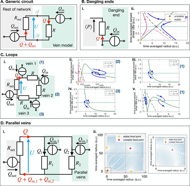
All circuits discussed in the text.

(A) General circuit for a vein connected to the rest of the network. (B) Dangling ends; (i) Electric circuit and notations and (ii) stability diagram in the shear radius space. (C) Loops; (i) Electric circuit and notations (ii) Stability diagram in the shear radius space for vein 2 and (**iii**) for veins 1 and 3. (D) Parallel Veins; (i) Electric circuit and notations (ii) Stability diagram in the radius - radius space.

Videos

Video 1

Download asset

posterframe for video — Bright field stacked images of the close-up specimen including veins #H, #I and #J in Figure 1A.i.

Frame sequence: 5 frames at 600 ms and 1 frame at 2.5 s. Scale 0.353 μm/pix.

Video 2

Download asset

Video 3

Download asset

Appendix 1—video 1

Download asset

Appendix 1—video 2

Download asset

Appendix 1—video 3

Download asset

Appendix 1—video 4

Download asset

Appendix 1—video 5

Download asset

Appendix 1—video 6

Download asset

Appendix 1—video 7

Download asset

Appendix 1—video 8

Download asset

Tables

Appendix 1—table 1

List of commonly used variables in our work in alphabetical order and significance.

Short length scale variations correspond to variables that can vary strongly from one vein to a neighboring vein, while long length scale variations vary smoothly throughout the network. Variables have short timescale variations when they have significant variations over timescales much smaller than the peristaltic contractions $T ≃ 1 - 2 \min$ ; and long timescale variations if they vary over longer timescales corresponding to vascular adaptation and rearrangement.

Variable	Significance	Length scale variations	Timescale variations
$a$	Radius of a vein	Short	Short and long
$ϵ$	Relative contraction amplitude	–	–
$L$	Length of a vein	–	–
$μ$	Inner fluid viscosity	Long	Long
$ω = 2 π / T$	Contraction frequency	–	–
$P$	Inner fluid pressure	Long	Short and long
$P_{0}$	Atmospheric pressure	–	–
$Q$	Fluid flow pervading a vein	Short	Short and long
$Q_{in}$	Fluid flow generated by peristaltic contractions in a vein	Short	Short and long
$Q_{net}$	Fluid flow generated by the rest of the network	Short	Short and long
$R$	Resistance of a vein, $R = 8 μ L / π a^{4}$	Short	Short and long
$R_{net}$	Resistance of the rest of the network attached to a vein at both vein ends	Short	Short and long
$τ$	Shear rate on a vein’s inner wall	Short	Short and long
$τ_{s}$	Sensed shear rate for adaptation	Short	Long
$τ_{0}$	Steady state shear rate, $τ_{0} \sim τ_{active} - ⟨ P - P_{0} ⟩ / μ$	Long	Long
$τ_{active}$	Active contribution to $τ_{0}$ , due to energetic consumption from the actomyosin cortex to maintain contractions	Long	Long
$t$	Time	–	–
$t_{adapt} ≃ 10 - 100 \min$	Long-time adaptation timescale	Long	Long
$t_{delay} ≃ 2 \min$	Delay between adaptation and shear rate	Long	Long
$T ≃ 1 - 2 \min$	Peristaltic contraction period	–	–
$⟨ X ⟩$	Long-time average of $X$	–	Long

Appendix 2—table 1

Summary of all fitting parameters of sample trajectories depicted in Appendix 2—figure 4, right-hand side.

These fits include fitting of $t_{d e l a y}$ . The fits are done over a range in time $t \in [t_{\min}, t_{\max}]$ .

Experiment	$t_{d e l a y} i n s$	$t_{a d a p t} i n s$	$τ_{0} i n s^{- 1}$	$t_{m i n} - t_{m a x} i n m i n$	$e r r o r ϵ_{e r r}$
data set G∗	69 ± 3	903 ± 190	5.4 ± 0.04	25–46	1.6 %
data set F∗	82 ± 3	335 ± 8	5.7 ± 0.03	90–102	0.17 %
data set E∗	352 ± 7	798 ± 3	3.07 ± 0.02	67–104	0.6 %
data set K∗	76 ± 4	85 ± 4	3.63 ± 0.01	50–90	2.7 %

Appendix 2—table 2

Summary of all fitting parameters with a fixed time delay of $t_{delay} = 120 s$ for the 12 close-up data sets.

Note that when a data set name is repeated, it corresponds to fitting results over different time ranges $t \in [t_{\min}, t_{\max}]$ for the same data set.

Experiment	$t_{a d a p t} i n s$	$τ_{loc} i n s^{- 1}$	$t_{m i n} - t_{m a x} i n m i n$	$e r r o r ϵ_{e r r}$
data set A	2682 ± 831	1.48 ± 0.17	0–17	0.13 %
data set A	220 ± 10	0.44 ± 0.00	17–33	0.22 %
data set A	246 ± 960	1.21 ± 0.59	67–83	0.68 %
data set B	1195 ± 20	1.43 ± 0.00	10–75	1.4 %
data set C	5948 ± 122	0.97 ± 0.00	0–83	1.9 %
data set D	1531 ± 69	0.58 ± 0.01	0–33	2.0 %
data set D	377 ± 6	0.79 ± 0.00	8–50	3.2 %
data set E	1312 ± 37	1.46 ± 0.01	0–21	0.93 %
data set E	1894 ± 49	3.05 ± 0.02	58–83	0.66 %
data set F	4323 ± 319	3.30 ± 0.06	0–42	1.9 %
data set F	4323 ± 319	3.30 ± 0.06	0–42	1.9 %
data set F	910 ± 24	5.08 ± 0.03	83–100	0.27 %
data set G	1153 ± 51	6.07 ± 0.04	12–29	0.38 %
data set G	1808 ± 322	1.00 ± 0.09	42–54	0.61 %
data set G	1233 ± 54	6.68 ± 0.07	83–100	0.31 %
data set H	355 ± 8	2.35 ± 0.02	0–25	1.4 %
data set I	274 ± 5	2.27 ± 0.01	0–25	1.6 %
data set J	601 ± 132	1.41 ± 0.09	0–25	3.1 %
data set K	278 ± 6	3.16 ± 0.00	8–67	2.0 %
data set K	85 ± 2	3.70 ± 0.00	45–75	0.6 %
data set K	862 ± 119	3.40 ± 0.13	67–108	1.5 %
data set K	123 ± 2	4.18 ± 0.00	108–133	0.53 %
data set L	2553 ± 248	0.27 ± 0.01	6–23	1.3 %

Appendix 2—table 3

Summary of fitted parameters for a 15 randomly selected veins in the full network Appendix 2—figure 6.

$t_{d e l a y}$ was established with cross-correlation, while $t_{a d a p t}$ and $τ_{0}$ were obtained through linear least-squares fitting. Error bars correspond to the 95% confidence interval and N.R. corresponds to non relevant points for which the 95% confidence interval yielded error bars as big as the parameters themselves and were, hence, deemed non-relevant.

Vein index in full network	$t_{d e l a y} i n s$	$t_{a d a p t} i n s$	$τ_{0} i n s^{- 1}$	$e r r o r ϵ_{e r r}$	$e r r o r ϵ_{e r r} w i t h t_{d e l a y} = 0$
a	24	1800 ± 250	0.76 ± 0.02	8.1%	7.9%
b	78	1520 ± 40	0.89 ± 0.02	2.6%	2.9%
c	360	1500 ± 150	N.R.	1.4%	1.4%
d	120	1800 ± 100	N.R.	17%	23%
e	120	900 ± 70	0.2 ± 0.05	7.4%	11%
f	186	2750 ± 100	0.38 ± 0.05	5.2%	6.3%
g	42	2450 ± 50	0.94 ± 0.03	5.0%	5.1%
h	246	N.R.	0.26 ± 0.03	8%	11%
i	186	870 ± 40	0.26 ± 0.01	3.3%	6.9%
j	54	2200 ± 100	1.1 ± 0.2	5.2%	5.0%
k	288	730 ± 50	4.0 ± 1.0	4.7%	6.7%
l	108	4050 ± 200	N.R.	1.1%	1.2%
m	360	10000 ± 3000	0.62 ± 0.1	6.1%	8.0%
n	18	2050 ± 200	0.73 ± 0.02	3.7%	3.8%
o	54	7300 ± 3000	0.48 ± 0.12	6.5%	6.8%

Additional files

MDAR checklist: https://cdn.elifesciences.org/articles/78100/elife-78100-mdarchecklist1-v2.docx
Download elife-78100-mdarchecklist1-v2.docx

Download links

A two-part list of links to download the article, or parts of the article, in various formats.

Downloads (link to download the article as PDF)

Article PDF

Open citations (links to open the citations from this article in various online reference manager services)

Mendeley

Cite this article (links to download the citations from this article in formats compatible with various reference manager tools)

Sophie Marbach
Noah Ziethen
Leonie Bastin
Felix K Bäuerle
Karen Alim

(2023)

Vein fate determined by flow-based but time-delayed integration of network architecture

eLife 12:e78100.

https://doi.org/10.7554/eLife.78100

Share this article

Cite this article

Diverse vein dynamics emerge during network reorganization.

Shear rate induces vein adaptation with a time delay.

Stable and unstable vein dynamics are predicted within the same model.

Feedback parameters integrate the network’s architecture and provide information on vein relative location.

Network architecture controls vein fate as exemplified in three cases.

Avalanche of sequentially vanishing veins.

Extracting average shear rates from shear rate data.

Vascular adaptation dynamics for all close up experiments, using time-averaged shear rates ⟨τ⟩ and time-averaged radius ⟨a⟩.

Vascular adaptation dynamics for a few veins in the full network #1 using time-averaged shear rates ⟨τ⟩ and time-averaged radius ⟨a⟩.

Additional data on the full network specimen #2.

Additional data on the full network specimen #3.

Cross correlation between average vein radius and different flow-based parameters (A) the connected resistance Rnet, (B) the relative resistance R/Rnet, (C) the vein outflow Q and (E) the local pressure ⟨P⟩.

Time delay extracted is independent of averaging technique or oscillation frequency.

Time delay statistics from full networks.

Time delays obtained with cross-correlation method on stable close-up data sets.

Evaluation of all three model parameters tadapt, tdelay and τ0 from suitable data sets (#E, #F, #G, #K).

Fit results graphical representation of model Equation 1 and Equation 2 using a fixed time delay of tdelay=120 s for all 12 close-up data sets on a given time window for each data set.

Fit results of model Equation 1 and Equation 2 for 15 randomly selected veins on specimen #1.

Principle of the calculation of Rnet on the basis of a few examples.

All circuits discussed in the text.

Bright field stacked images of the close-up specimen including veins #H, #I and #J in Figure 1A.i.

Bright field stacked images of the close-up specimen including vein #K in Figure 1A.ii.

Bright field stacked images of the full network specimen #1 in Figure 1B.i.

Bright field stacked images of the close-up specimen including vein #A.

Bright field stacked images of the close-up specimen including vein #B.

Bright field stacked images of the close-up specimen including vein #C.

Bright field stacked images of the close-up specimen including vein #D.

Bright field stacked images of the close-up specimen including vein #E, #F and #G.

Bright field stacked images of the close-up specimen including vein #L.

Bright field stacked images of the full network specimen #2.

Bright field stacked images of the full network specimen #3.

List of commonly used variables in our work in alphabetical order and significance.

Summary of all fitting parameters of sample trajectories depicted in Appendix 2—figure 4, right-hand side.

Summary of all fitting parameters with a fixed time delay of tdelay=120s for the 12 close-up data sets.

Summary of fitted parameters for a 15 randomly selected veins in the full network Appendix 2—figure 6.

MDAR checklist

Downloads (link to download the article as PDF)

Open citations (links to open the citations from this article in various online reference manager services)

Cite this article (links to download the citations from this article in formats compatible with various reference manager tools)

Vascular adaptation dynamics for all close up experiments, using time-averaged shear rates $⟨ τ ⟩$ and time-averaged radius $⟨ a ⟩$ .

Vascular adaptation dynamics for a few veins in the full network #1 using time-averaged shear rates $⟨ τ ⟩$ and time-averaged radius $⟨ a ⟩$ .

Cross correlation between average vein radius and different flow-based parameters (A) the connected resistance $R_{net}$ , (B) the relative resistance $R / R_{net}$ , (C) the vein outflow $Q$ and (E) the local pressure $⟨ P ⟩$ .

Evaluation of all three model parameters $t_{a d a p t}$ , $t_{d e l a y}$ and $τ_{0}$ from suitable data sets (#E, #F, #G, #K).

Fit results graphical representation of model Equation 1 and Equation 2 using a fixed time delay of $t_{d e l a y} = 120 s$ for all 12 close-up data sets on a given time window for each data set.

Principle of the calculation of $R_{net}$ on the basis of a few examples.

Summary of all fitting parameters with a fixed time delay of $t_{delay} = 120 s$ for the 12 close-up data sets.