Tools and Resources

Cancer Biology

Robust and Efficient Assessment of Potency (REAP) as a quantitative tool for dose-response curve estimation

Department of Public Health Sciences, Pennsylvania State University, United States
Department of Lymphoma and Myeloma, University of Texas MD Anderson Cancer Center, United States
Department of Pharmacology, Pennsylvania State University, United States
Department of Pediatrics, Pennsylvania State University, United States
Department of Biochemistry and Molecular Biology, Pennsylvania State University, United States
Department of Surgery, The Pennsylvania State University, United States
Department of Biostatistics, University of Texas MD Anderson Cancer Center, United States

Aug 3, 2022

https://doi.org/10.7554/eLife.78634

Open access
Copyright information

Figures
Tables
Additional files

7 figures, 4 tables and 1 additional file

Figures

Figure 1

Download asset Open asset

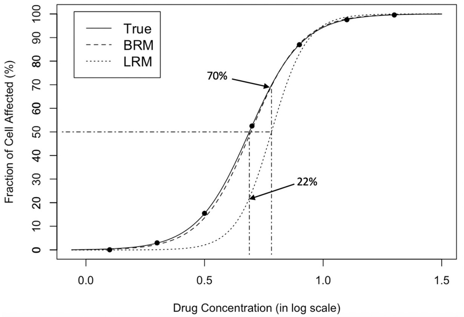
Dose-response curve fitting with extreme observations.

The original data points are on the true curve. The leftmost data point is changed from 0.005 to 1e-6, referring to a small white noise that cannot be visually recognized. The change leads to the obvious departure between the estimated curve by linear regression model (dotted) and the true curve (solid), which demonstrates that standard regression is sensitive to extreme values. The response at the true IC₅₀ (dotdashed, vertical, left) is only 22% from the estimated curve; the estimated IC₅₀ (dotdashed, vertical, right) corresponds to the 70% fraction of cell affected, effecting a substantive 20% inflation (50% ->70%) in estimation error. In contrast, the estimated curve by beta regression model (dashed) is almost overlapped with the true curve (solid), which shows that BRM is much more robust to extreme values. LRM: linear regression model; BRM: robust beta regression model. Detailed model descriptions of LRM and BRM are provided in Materials and methods section.

Figure 2

Download asset Open asset

Comparison of estimation efficiency and accuracy using linear regression model and beta regression model.

Deleting the extreme values could not eliminate the bias (panel A), but only harmed the accuracy with worse coverage probabilities (panel B) and impaired the efficiency of interval estimation with wider nominal 95% confidence intervals (panel C). A total of 1000 data sets were generated following the data simulating process described in **Appendix 1**, using the dose sets and true dose-response curve under 7 dose setting with a precision parameter of 100. Responses ≤5% or ≥95% were considered extreme responses. Dashed line in panel B denotes 95% nominal coverage probability. BRM: beta regression with extreme data points; LRM: linear regression model with extreme data points; LRM(t): linear regression model with truncated dataset after deleting extreme values. Detailed model descriptions of LRM and BRM are provided in Materials and methods section.

Figure 3

Download asset Open asset

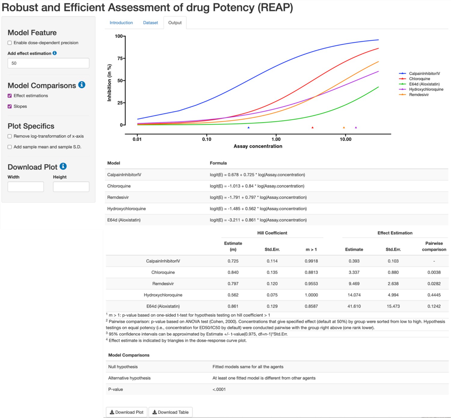
REAP App interface, with a highlight of Output section.

Using the robust beta regression method, REAP produces a dose-response curve plot with effect and model estimations. The left panel allows users to specify model features and design plot specifics. REAP also provides hypothesis testing results to compare effect estimations, slopes and models.

Figure 4

Download asset Open asset

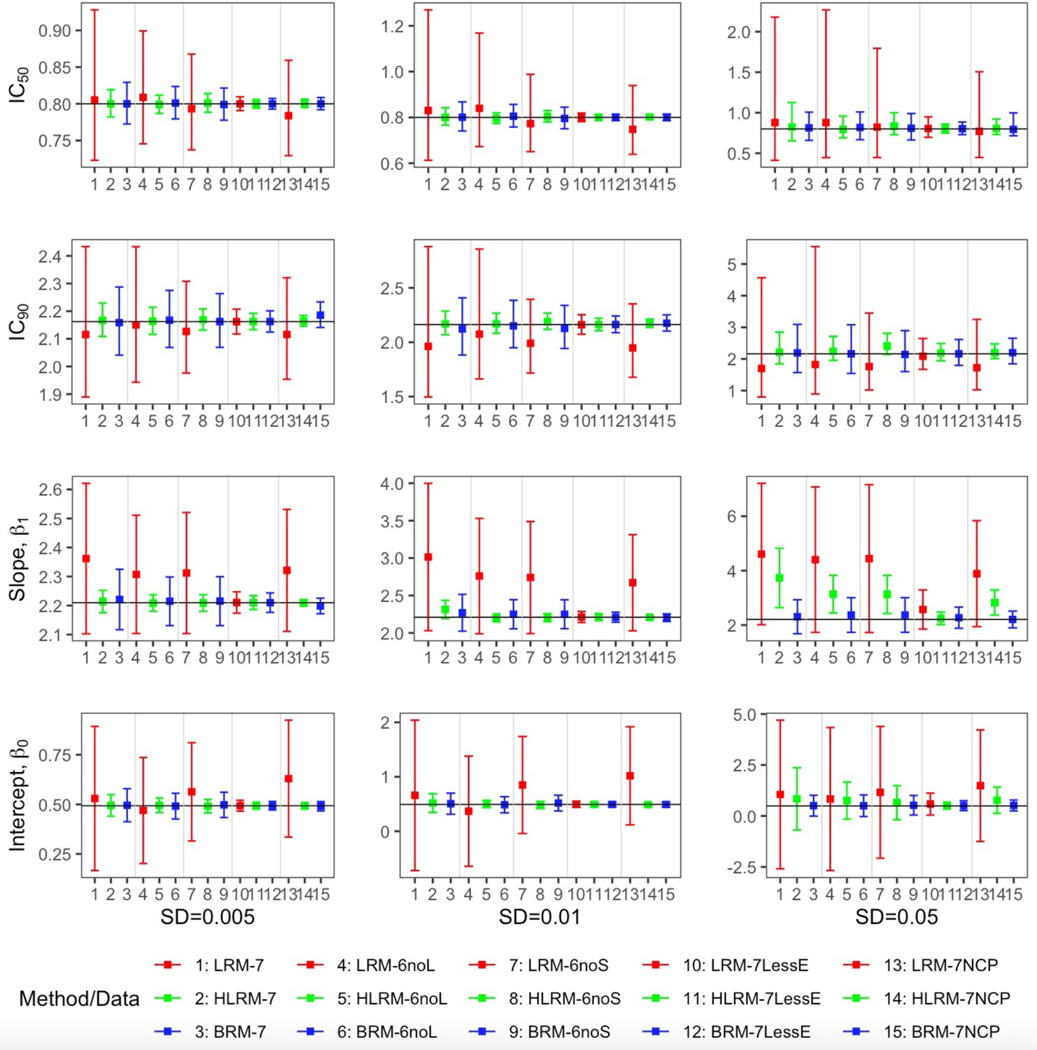
Comparison of the point estimates and 95% confidence intervals using linear regression model, heavy-tailed linear regression model and robust beta regression model, with data simulated from normal error term.

The vertical solid lines indicate the true values. The dots represent the averaged point estimates and the bars represent the averaged lower and upper bound of 95% CIs. The point estimation by robust beta regression is consistently closer to the true value with a narrower 95% CI compared to the linear regression model. The 95% CI of heavy-tailed linear regression underestimates the nominal coverage probability. LRM: linear regression model; LRM-7: LRM under 7-dose dataset with extreme data points; LRM-6noL: LRM under 6 dose dataset after removing the highest dose data point; LRM-6noS: LRM under 6-dose dataset after removing the lowest dose data point; LRM-7lessE: LRM under 7-dose dataset with less extreme data points; LRM-7NCP: LRM under 7-dose dataset with extreme data points and dose-dependent precision; HLRM: heavy-tailed linear regression model; HLRM-7: Heavy-tailed LRM under 7-dose dataset with extreme data points; HLRM-6noL: Heavy-tailed LRM under 6-dose dataset after removing the highest dose data point; HLRM-6noS: Heavy-tailed LRM under 6-dose dataset after removing the lowest dose data point; HLRM-7lessE: Heavy-tailed LRM under 7-dose dataset with less extreme data points; HLRM-7NCP: Heavy-tailed LRM under 7-dose dataset with extreme data points and dose-dependent precision; BRM: robust beta regression model; BRM-7: BRM under 7-dose dataset with extreme data points; BRM-6noL: BRM under 6-dose dataset after removing the highest dose data point; BRM-6noS: BRM under 6-dose dataset after removing the lowest dose data point; BRM-7lessE: BRM under 7-dose dataset with less extreme data points; BRM-7NCP: BRM under 7-dose dataset with extreme data points and dose-dependent precision. Detailed model descriptions of LRM, HLRM, and BRM are provided in Materials and methods section.

Figure 5

Download asset Open asset

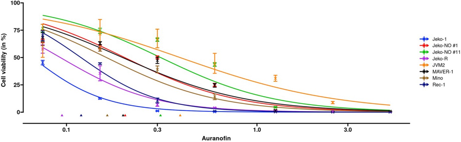
Dose-response curve estimation of auranofin (μM) under different MCL cell lines.

The dose-response curve was fitted with a dose-dependent precision with $l o g (d o s e)$ as an additional regressor for the precision estimator. Observed dose effects are displayed with interval bars, which end with arrows when estimated intervals exceed (0,1). Triangles at the bottom indicate IC₅₀ values for each MCL cell line. MCL: mantle cell lymphoma.

Figure 6

Download asset Open asset

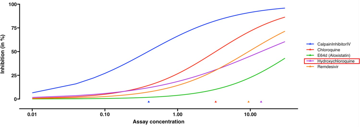
Dose-response curve estimation of anti-viral drugs under the same biological batch with SARS-CoV-2 data.

The robust beta regression gives reasonable estimations to the dose-response curve of hydroxychloroquine, compared to the inconclusive dose-response curve fitted by linear regression in Bobrowski et al. (2020). The plot is generated without selecting the option of mean and confidence interval for observations. Triangles indicate the estimated EC₅₀ values for each drug.

Appendix 1—figure 1

Download asset Open asset

Tables

Appendix 1—table 1

Simulation result of bias, RMSE and 95% CI coverage probability corresponding to normal error terms.

Scenario	Method	Bias				RMSE				95% CI Coverage Probability
		IC₅₀	IC₉₀	$β_{0}$	$β_{1}$	IC₅₀	IC₉₀	$β_{0}$	$β_{1}$	IC₅₀	IC₉₀	$β_{0}$	$β_{1}$
(a)data simulated using normal error term with SD = 0.005
7 doses with extreme values	LRM	0.005	–0.047	0.037	0.152	0.098	0.298	0.525	0.557	0.954	0.773	0.943	0.666
	HLRM	0.000	0.004	0.002	0.004	0.018	0.102	0.063	0.169	0.468	0.335	0.463	0.225
	BRM	0.000	–0.004	0.003	0.011	0.013	0.130	0.044	0.088	0.981	0.927	0.975	0.889
6 doses after removing largest	LRM	0.009	–0.01	–0.024	0.098	0.045	0.184	0.129	0.517	0.967	0.921	0.971	0.691
	HLRM	–0.001	0.001	0.002	–0.001	0.014	0.063	0.037	0.065	0.453	0.408	0.467	0.250
	BRM	0.001	0.005	–0.00	0.005	0.009	0.132	0.024	0.089	0.955	0.892	0.950	0.844
6 doses after removing smallest	LRM	–0.007	–0.036	0.070	0.102	0.037	0.306	0.362	0.533	0.969	0.623	0.933	0.695
	HLRM	0.001	0.007	–0.002	–0.001	0.014	0.083	0.046	0.064	0.456	0.249	0.400	0.259
	BRM	–0.001	0.000	0.005	0.005	0.009	0.151	0.039	0.089	0.956	0.872	0.940	0.853
7 doses with less extreme values	LRM	0.000	–0.000	0.000	0.001	0.005	0.030	0.016	0.026	0.891	0.828	0.883	0.799
	HLRM	0.000	0.000	0.000	0.000	0.005	0.031	0.016	0.028	0.668	0.599	0.661	0.567
	BRM	0.000	0.000	0.000	0.000	0.004	0.026	0.013	0.024	0.864	0.823	0.860	0.800
7 doses with extreme values and dose-dependent precision	LRM	–0.016	–0.047	0.137	0.111	0.069	0.409	0.583	0.520	0.965	0.573	0.921	0.685
	HLRM	0.000	0.003	–0.001	–0.001	0.008	0.049	0.027	0.036	0.325	0.188	0.290	0.151
	BRM	0.000	0.023	–0.003	–0.011	0.003	0.196	0.023	0.095	0.957	0.849	0.931	0.794
(b)data simulated using normal error term with SD = 0.01
7 doses with extreme values	LRM	0.030	–0.200	0.166	0.804	0.224	0.544	1.234	1.305	0.958	0.699	0.950	0.716
	HLRM	0.000	0.006	0.025	0.105	0.031	0.238	0.199	0.795	0.408	0.286	0.404	0.194
	BRM	0.001	–0.039	0.013	0.060	0.030	0.172	0.094	0.155	0.981	0.931	0.976	0.892
6 doses after removing largest	LRM	0.040	–0.088	–0.125	0.549	0.101	0.280	0.314	1.245	0.966	0.924	0.972	0.734
	HLRM	–0.004	0.007	0.008	–0.008	0.027	0.125	0.075	0.123	0.424	0.384	0.445	0.241
	BRM	0.005	–0.012	–0.007	0.040	0.019	0.140	0.044	0.148	0.954	0.893	0.949	0.850
6 doses after removing smallest	LRM	–0.027	–0.172	0.357	0.531	0.080	0.534	0.836	1.220	0.966	0.561	0.937	0.734
	HLRM	0.004	0.027	–0.010	–0.005	0.028	0.160	0.089	0.125	0.434	0.247	0.384	0.253
	BRM	–0.005	–0.035	0.025	0.040	0.018	0.178	0.078	0.143	0.958	0.877	0.943	0.857
7 doses with less extreme values	LRM	0.000	–0.001	0.001	0.004	0.011	0.060	0.032	0.053	0.892	0.826	0.883	0.799
	HLRM	0.000	0.000	0.001	0.002	0.011	0.061	0.032	0.056	0.665	0.597	0.657	0.564
	BRM	0.000	0.001	0.000	0.001	0.009	0.052	0.026	0.048	0.865	0.822	0.860	0.801
7 doses with extreme values and dose-dependent precision	LRM	–0.052	–0.215	0.524	0.462	0.130	0.622	1.123	0.984	0.965	0.521	0.921	0.726
	HLRM	0.002	0.011	–0.004	–0.003	0.016	0.096	0.053	0.071	0.303	0.180	0.273	0.148
	BRM	0.000	0.012	–0.001	–0.005	0.009	0.142	0.054	0.080	0.957	0.851	0.932	0.798
(c)data simulated using normal error term with SD = 0.05
7 doses with extreme values	LRM	0.079	–0.463	0.560	2.399	0.393	0.924	2.128	1.853	0.948	0.612	0.942	0.591
	HLRM	0.024	0.047	0.345	1.524	0.223	1.050	1.600	2.638	0.477	0.258	0.447	0.083
	BRM	0.013	0.029	0.010	0.095	0.129	0.524	0.371	0.377	0.857	0.861	0.869	0.855
6 doses after removing largest	LRM	0.079	–0.338	0.337	2.194	0.276	0.749	2.054	2.239	0.968	0.779	0.975	0.675
	HLRM	–0.005	0.080	0.260	0.926	0.170	0.820	1.392	2.547	0.407	0.293	0.417	0.146
	BRM	0.017	0.001	0.007	0.160	0.124	0.512	0.387	0.430	0.879	0.835	0.912	0.812
6 doses after removing smallest	LRM	0.022	–0.403	0.666	2.232	0.335	0.965	1.936	2.220	0.972	0.610	0.898	0.681
	HLRM	0.035	0.244	0.162	0.919	0.158	0.998	1.332	2.526	0.410	0.209	0.320	0.146
	BRM	0.009	–0.021	0.030	0.160	0.119	0.511	0.358	0.420	0.874	0.754	0.862	0.819
7 doses with less extreme values	LRM	0.005	–0.077	0.086	0.362	0.084	0.383	0.693	1.215	0.905	0.795	0.895	0.813
	HLRM	0.001	0.029	0.009	0.039	0.053	0.327	0.185	0.446	0.619	0.551	0.610	0.520
	BRM	0.002	–0.001	0.012	0.062	0.054	0.296	0.187	0.311	0.861	0.810	0.858	0.815
7 doses with extreme values and dose-dependent precision	LRM	–0.029	–0.441	0.994	1.679	0.297	0.955	1.840	1.715	0.945	0.444	0.904	0.678
	HLRM	0.006	0.037	0.278	0.617	0.106	0.710	1.152	1.781	0.335	0.145	0.295	0.105
	BRM	–0.005	0.037	0.023	–0.002	0.040	0.323	0.172	0.271	0.954	0.819	0.930	0.758

Appendix 1—table 2

Simulation result of bias, RMSE and 95% CI coverage probability corresponding to beta error terms.

Scenario	Method	Bias				RMSE				95% CI Coverage Probability
		IC₅₀	IC₉₀	$β_{0}$	$β_{1}$	IC₅₀	IC₉₀	$β_{0}$	$β_{1}$	IC₅₀	IC₉₀	$β_{0}$	$β_{1}$
(a)data simulated using beta error term with ϕ=35
7 doses with extreme values	LRM	0.017	–0.304	0.142	0.653	0.163	0.481	0.658	0.686	0.924	0.697	0.909	0.566
	HLRM	0.008	–0.161	0.085	0.366	0.117	0.478	0.402	0.576	0.581	0.429	0.571	0.313
	BRM	0.003	–0.014	0.018	0.073	0.074	0.339	0.219	0.275	0.835	0.818	0.832	0.829
6 doses after removing largest	LRM	0.039	–0.174	–0.027	0.504	0.115	0.402	0.354	0.666	0.933	0.864	0.936	0.666
	HLRM	0.015	–0.092	0.026	0.273	0.109	0.463	0.337	0.486	0.581	0.518	0.594	0.368
	BRM	0.008	0.005	0.007	0.077	0.077	0.375	0.229	0.298	0.812	0.808	0.811	0.803
6 doses after removing smallest	LRM	–0.022	–0.288	0.248	0.502	0.108	0.501	0.499	0.670	0.930	0.620	0.901	0.664
	HLRM	0.000	–0.120	0.094	0.274	0.106	0.509	0.366	0.487	0.596	0.383	0.547	0.368
	BRM	–0.002	–0.020	0.031	0.074	0.075	0.353	0.223	0.298	0.815	0.782	0.805	0.800
7 doses with less extreme values	LRM	0.004	–0.045	0.023	0.117	0.063	0.332	0.195	0.300	0.900	0.828	0.891	0.821
	HLRM	0.003	–0.017	0.021	0.096	0.067	0.382	0.205	0.323	0.686	0.630	0.680	0.619
	BRM	0.003	0.031	0.004	0.028	0.058	0.331	0.170	0.272	0.845	0.837	0.847	0.838
7 doses with extreme values and dose-dependent precision	LRM	0.080	–0.093	–0.179	0.444	0.147	0.281	0.435	0.548	0.904	0.908	0.927	0.639
	HLRM	0.061	–0.200	–0.063	0.753	0.199	0.553	0.676	0.967	0.484	0.447	0.520	0.231
	BRM	0.003	0.031	–0.003	0.012	0.067	0.277	0.182	0.236	0.755	0.780	0.768	0.772
(b)data simulated using beta error term with ϕ=15
7 doses with extreme values	LRM	0.029	–0.571	0.373	1.633	0.233	0.555	1.177	1.197	0.941	0.588	0.910	0.406
	HLRM	0.016	–0.334	0.225	0.983	0.172	0.657	0.725	1.186	0.561	0.353	0.544	0.213
	BRM	0.008	–0.050	0.036	0.174	0.109	0.464	0.324	0.403	0.817	0.790	0.820	0.805
6 doses after removing largest	LRM	0.074	–0.360	–0.043	1.269	0.164	0.516	0.635	1.192	0.942	0.823	0.939	0.556
	HLRM	0.029	–0.206	0.086	0.702	0.164	0.715	0.594	0.925	0.552	0.445	0.551	0.272
	BRM	0.018	–0.028	0.019	0.203	0.117	0.527	0.355	0.446	0.778	0.783	0.794	0.776
6 doses after removing smallest	LRM	–0.042	–0.564	0.620	1.280	0.157	0.596	0.890	1.180	0.939	0.503	0.905	0.555
	HLRM	–0.001	–0.262	0.237	0.700	0.160	0.712	0.663	0.917	0.546	0.300	0.486	0.268
	BRM	–0.001	–0.071	0.066	0.192	0.115	0.499	0.345	0.449	0.787	0.733	0.782	0.777
7 doses with less extreme values	LRM	0.008	–0.104	0.059	0.286	0.096	0.513	0.320	0.489	0.906	0.795	0.884	0.807
	HLRM	0.009	–0.030	0.048	0.240	0.103	0.726	0.325	0.517	0.694	0.602	0.678	0.598
	BRM	0.006	0.074	0.012	0.062	0.088	0.553	0.260	0.409	0.838	0.836	0.841	0.847
7 doses with extreme values and dose-dependent precision	LRM	0.165	–0.202	–0.425	1.114	0.218	0.374	0.771	0.959	0.916	0.886	0.941	0.534
	HLRM	0.141	–0.347	–0.250	2.055	0.291	1.027	1.270	1.798	0.515	0.440	0.576	0.136
	BRM	0.010	0.053	–0.008	0.050	0.104	0.423	0.281	0.368	0.763	0.790	0.764	0.769
(c)data simulated using beta error term with ϕ=5
7 doses with extreme values	LRM	0.042	–0.851	0.748	3.414	0.270	0.527	1.611	1.421	0.948	0.423	0.898	0.198
	HLRM	0.040	–0.629	0.689	3.147	0.278	1.518	1.480	2.112	0.681	0.241	0.644	0.094
	BRM	0.008	–0.011	0.047	0.191	0.161	0.606	0.589	0.767	0.811	0.800	0.815	0.811
6 doses after removing largest	LRM	0.106	–0.636	0.181	2.962	0.234	0.865	1.401	1.604	0.949	0.684	0.938	0.356
	HRLM	0.075	–0.098	0.276	2.410	0.274	8.599	1.351	2.082	0.607	0.362	0.600	0.142
	BRM	0.007	–0.115	0.112	0.355	0.166	0.643	0.621	0.761	0.762	0.752	0.773	0.769
6 doses after removing smallest	LRM	–0.039	–0.871	1.126	2.935	0.231	0.649	1.428	1.620	0.953	0.380	0.883	0.362
	HLRM	0.004	–0.371	0.773	2.379	0.261	5.238	1.464	2.068	0.599	0.206	0.492	0.149
	BRM	0.008	–0.087	0.070	0.328	0.166	0.588	0.509	0.724	0.766	0.755	0.772	0.773
7 doses with less extreme values	LRM	0.008	–0.456	0.275	1.126	0.152	0.515	0.679	1.041	0.915	0.639	0.874	0.707
	HLRM	0.007	–0.315	0.236	0.923	0.164	0.767	0.651	1.047	0.681	0.475	0.644	0.491
	BRM	0.002	–0.088	0.093	0.318	0.132	0.588	0.423	0.660	0.839	0.812	0.834	0.835
7 doses with extreme values and dose-dependent precision	LRM	0.245	–0.378	–0.646	2.300	0.274	0.470	1.207	1.262	0.908	0.833	0.947	0.343
	HLRM	0.209	–0.578	–0.233	4.982	0.332	6.852	2.016	2.017	0.683	0.381	0.728	0.050
	BRM	0.025	0.171	–0.032	0.074	0.161	0.762	0.426	0.549	0.757	0.796	0.761	0.770

Appendix 1—table 3

The first example of REAP application with B-cell lymphoma data, corresponding with Figure 5.

IC₅₀ estimations are ranked from low to high. Hypothesis testings on equal potency (i.e., concentration for IC₅₀) were conducted pairwise with the group right above (one rank lower). Jeko-1 has the highest potency and the difference of IC₅₀ estimations between Jeko-1 and Jeko-R is significant with a P-value <0.0001. The B-cell lymphoma dataset is available on Github (Fang et al., 2022).

Model	Intercept	Slope (m)	Std. Err for m	P-value for m>1	IC₅₀ estimation	Std. Err for IC₅₀ estimation	Pairwise comparison
Jeko-1	–4.807	–1.252	0.155	0.0519	0.021	0.008	-
Jeko-R	–4.305	–1.822	0.112	<.0001	0.094	0.006	<0.0001
Rec-1	–5.304	–2.63	0.091	<.0001	0.133	0.004	<0.0001
Mino	–2.684	–1.474	0.141	0.0004	0.162	0.015	0.0656
Jeko-NO #1	–2.012	–1.192	0.135	0.0769	0.185	0.021	0.3755
MAVER-1	–2.21	–1.37	0.125	0.0015	0.199	0.021	0.6312
Jeko-NO #11	–1.459	–1.267	0.152	0.0398	0.316	0.038	0.0114
JVM2	–1.056	–1.271	0.135	0.0223	0.436	0.055	0.0818

Appendix 1—table 4

The output for the estimated dose-response curve of anti-viral drugs under the same biological batch with SARS-CoV-2 data.

Calpain inhibitor IV has the highest potency (P-value = 0.0038). The reconstructed SARS-CoV-2 dataset is available on Github (Fang et al., 2022).

Model	Intercept	Slope (m)	Std. Err for m	P-value for m>1	EC₅₀ estimation	Std. Err for EC₅₀ estimation	Pairwise comparison
CalpainInhibitorIV	0.678	0.725	0.114	0.9918	0.393	0.103	-
Chloroquine	–1.013	0.84	0.135	0.8813	3.337	0.88	0.0038
Remdesivir	–1.791	0.797	0.12	0.9553	9.469	2.638	0.0282
Hydroxychloroquine	–1.485	0.562	0.075	1	14.074	4.994	0.4445
E64d (Aloxistatin)	–3.211	0.861	0.129	0.8587	41.61	15.473	0.1242

Additional files

MDAR checklist: https://cdn.elifesciences.org/articles/78634/elife-78634-mdarchecklist1-v1.docx
Download elife-78634-mdarchecklist1-v1.docx

Download links

A two-part list of links to download the article, or parts of the article, in various formats.

Downloads (link to download the article as PDF)

Article PDF

Open citations (links to open the citations from this article in various online reference manager services)

Mendeley

Cite this article (links to download the citations from this article in formats compatible with various reference manager tools)

Shouhao Zhou
Xinyi Liu
Xinying Fang
Vernon M Chinchilli
Michael Wang
Hong-Gang Wang
Nikolay V Dokholyan
Chan Shen
J Jack Lee

(2022)

Robust and Efficient Assessment of Potency (REAP) as a quantitative tool for dose-response curve estimation

eLife 11:e78634.

https://doi.org/10.7554/eLife.78634

Figures

Dose-response curve fitting with extreme observations.

Comparison of estimation efficiency and accuracy using linear regression model and beta regression model.

REAP App interface, with a highlight of Output section.

Comparison of the point estimates and 95% confidence intervals using linear regression model, heavy-tailed linear regression model and robust beta regression model, with data simulated from normal error term.

Dose-response curve estimation of auranofin (μM) under different MCL cell lines.

Dose-response curve estimation of anti-viral drugs under the same biological batch with SARS-CoV-2 data.

Comparison of the point estimates and 95% confidence intervals using linear regression model, heavy-tailed linear regression model and robust beta regression model, with data simulated from beta error term.

Tables

Simulation result of bias, RMSE and 95% CI coverage probability corresponding to normal error terms.

Simulation result of bias, RMSE and 95% CI coverage probability corresponding to beta error terms.

The first example of REAP application with B-cell lymphoma data, corresponding with Figure 5.

The output for the estimated dose-response curve of anti-viral drugs under the same biological batch with SARS-CoV-2 data.

Additional files

MDAR checklist

Download links

Downloads (link to download the article as PDF)

Open citations (links to open the citations from this article in various online reference manager services)

Cite this article (links to download the citations from this article in formats compatible with various reference manager tools)

Be the first to read new articles from eLife

Share this article

Cite this article

Dose-response curve fitting with extreme observations.

Comparison of estimation efficiency and accuracy using linear regression model and beta regression model.

REAP App interface, with a highlight of Output section.

Comparison of the point estimates and 95% confidence intervals using linear regression model, heavy-tailed linear regression model and robust beta regression model, with data simulated from normal error term.

Dose-response curve estimation of auranofin (μM) under different MCL cell lines.

Dose-response curve estimation of anti-viral drugs under the same biological batch with SARS-CoV-2 data.

Comparison of the point estimates and 95% confidence intervals using linear regression model, heavy-tailed linear regression model and robust beta regression model, with data simulated from beta error term.

Simulation result of bias, RMSE and 95% CI coverage probability corresponding to normal error terms.

Simulation result of bias, RMSE and 95% CI coverage probability corresponding to beta error terms.

The first example of REAP application with B-cell lymphoma data, corresponding with Figure 5.

The output for the estimated dose-response curve of anti-viral drugs under the same biological batch with SARS-CoV-2 data.

MDAR checklist

Downloads (link to download the article as PDF)

Open citations (links to open the citations from this article in various online reference manager services)

Cite this article (links to download the citations from this article in formats compatible with various reference manager tools)