Ultrafast simulation of large-scale neocortical microcircuitry with biophysically realistic neurons
- Department of Cell Biology, Emory University School of Medicine, United States
- Department of Neurology, Emory University School of Medicine, United States
Figures
Figure 1 with 1 supplement
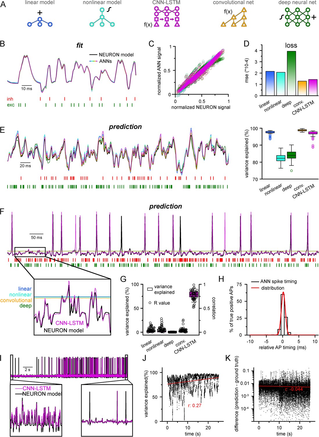
Single-compartmental neuronal simulations using artificial neural networks (ANNs).
(A) Representative diagrams of the tested architectures, outlining the ordering of the specific functional blocks of the ANNs. (B) Continuous representative trace of a point-by-point fit of passive membrane potential. (C) Point-by-point fit plotted against ground truth data (n = 45,000). (D) Mean squared error of ANN fits corresponds to the entire training dataset (n = 2.64 * 106 datapoints). Single quantal inputs arrive stochastically with a fixed quantal size: 2.5 nS for excitatory, 8 nS for inhibitory inputs, sampling is 1 kHz. Red and green bars below membrane potential traces denote the arrival of inhibitory and excitatory events, respectively. (E) Representative trace of a continuous passive membrane potential prediction (left) created by relying on past model predictions. Explained variance (right) was calculated from 500-ms-long continuous predictions (n = 50). (F) Representative active membrane potential prediction by ANNs. (G) Explained variance (box chart) and Pearson’s r (circles) of model predictions and ground truth data for the five ANNs from 50 continuous predictions, 500 ms long each. (H) Spike timing of the convolutional neural network-long short-term memory (CNN-LSTM) model calculated from the same dataset as panel (G). Color coding is the same as in panel (A). (I) Representative continuous, 25-s-long simulation of subthreshold and spiking activity. (J) Explained variance as a function of time during the 25-s-long simulation depicted in panel (I). Red line and r-value correspond to the best linear fit. (K) Difference between voltage traces produced by NEURON and ANN simulations. Red line and r-value correspond to the best linear fit.
Figure 1—figure supplement 1

Convolutional neural network-long short-term memory (CNN-LSTM) architecture for time-series forecasting.
The input of the artificial neural network (ANN) consisted of a membrane potential vector (Vm) and the weights and onsets of synaptic inputs (a representative inhibitory synapse, inh in red; and an excitatory synapse, exc in green). The first layer of the ANN (Conv1D) creates a temporally aligned convolved representation (colored bars) of the input by sliding a convolutional kernel (gray box) along the input. The second functional block (LSTM layers) processes the output of the convolutional layers through recurrent connections to weigh information temporally. The last functional block consisting of fully connected layers provides additional nonlinear information processing power. The output of the network in this case is the first subsequent Vm value (tn+1). The number of layers belonging to specific functional blocks of the CNN-LSTM architecture may vary. Red and green bars below membrane potential traces denote the arrival of inhibitory and excitatory events, respectively.
Figure 2
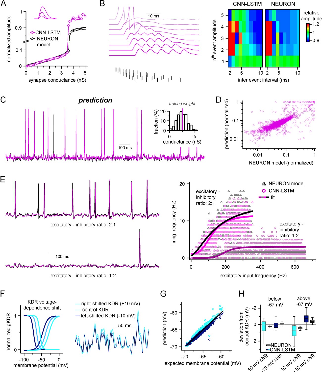
Ideal generalization of the convolutional neural network-long short-term memory (CNN-LSTM).
(A) CNN-LSTM models predict similar subthreshold event amplitudes and action potential threshold (break in y-axis) for increasing input weight, compared to NEURON models. (B) CNN-LSTM models correctly represent temporal summation of synaptic events. Representative traces for different inter-event intervals (range: 2–10 ms, 1 ms increment) on the left, comparison of individual events in a stimulus train, relative to the amplitude of unitary events on the right. (C) Single-simulated active membrane potential trace in CNN-LSTM (purple) and NEURON (black) with variable synaptic input weights (left). The inset shows the distribution of synaptic weights used for testing generalization, with the original trained synaptic weight in purple. CNN-LSTM predicted membrane potential values plotted against NEURON model ground truth (right). Plotted values correspond to continuously predicted CNN-LSTM traces. (D) CNN-LSTM model predictions are accurate in various synaptic environments. Firing frequency was quantified upon two different excitation–inhibition ratios (2:1 – representative top trace on the left and bright magenta circles on the right, 1:2 – representative bottom trace on the left and dark magenta circles on the right). (E) Subthreshold effects of potassium conductance biophysical alterations are correctly depicted by the CNN-LSTM. Voltage dependence of the delayed rectifier conductances is illustrated on the left and their effect on subthreshold membrane potential is shown on the right (control conditions are shown in blue, 10 mV left-shifted delayed rectifier conditions in navy blue and 10 mV right-shifted conditions are shown in teal). (F) CNN-LSTM membrane potential predictions for left- (navy) or right-shifted potassium conditions are compared to control conditions., Membrane potential responses below and above –67 mV are quantified for the two altered potassium conductances in NEURON simulation and CNN-LSTM predictions. The effects of biophysical changes of potassium channels were only apparent at membrane potentials above their activation threshold (–67 mV). (G) Artificial neural networks (ANNs) fitting NEURON models with left-shifted (dark blue) and right-shifted (light blue) KDR conductances are plotted against membrane potential responses of ANNs with control KDR conductances. The separation of the two responses shows voltage response modulation of KDR at subthreshold membrane potentials. (H) Membrane potential responses of NEURON and ANN models below and above resting membrane potential (–67 mV).
Figure 3

Convolutional neural network-long short-term memory (CNN-LSTM) prediction of neuronal mechanisms beyond somatic membrane potential.
(A) Representative membrane potential (Vm, top) and ionic current (IK, potassium current; Ina, sodium current, bottom) dynamics prediction upon arriving excitatory (green, middle) and inhibitory (red, middle) events. Enlarged trace shows subthreshold voltage and current predictions. Color coding is same as for Figure 1. (black, NEURON model traces; magenta, CNN-LSMT; blue, linear model; teal, nonlinear model; green, deep neural net; orange, convolutional net). Notice the smooth vertical line corresponding to predictions by artificial neural networks (ANNs), with the exception of CNN-LSTM. On bottom left, magnified view illustrates the subthreshold correspondence of membrane potential and ionic current traces. (B) CNN-LSTM models accurately predict ionic current dynamics. Normalized ANN predictions are plotted against normalized neuron signals for sodium (dark gray, left) and potassium currents (light gray). (C) Variance of suprathreshold traces is largely explained by CNN-LSTM predictions (right, color coding is same as in panel [B], left). Correlation coefficients are superimposed in black.
Figure 4
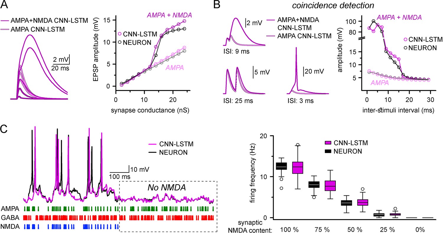
Accurate representation of nonlinear synaptic activation by convolutional neural network-long short-term memory (CNN-LSTM).
(A) Representative synaptic responses with variable synaptic activation, CNN-simulated AMPA receptors (light magenta) and AMPA + NMDA receptors (magenta), on the left. AMPA + NMDA response amplitudes nonlinearly depend on the activated synaptic conductance (magenta, CNN-LSTM; black, NEURON), compared to AMPA responses (light magenta, CNN-LSTM; gray, NEURON), on the right. (B) NMDA response nonlinearity enables coincidence detection in a narrow time window, resulting in action potential (AP) generation at short stimulus intervals. (C). Neuronal output modulation is dependent on synaptic NMDA receptor content in a naturalistic network condition. Representative traces on the left (CNN-LSTM, magenta; NEURON, black). Summary depiction of firing frequencies with varying amounts of NMDA receptor activation (percentages denominate the synaptic NMDA-AMPA fraction).
Figure 5 with 3 supplements
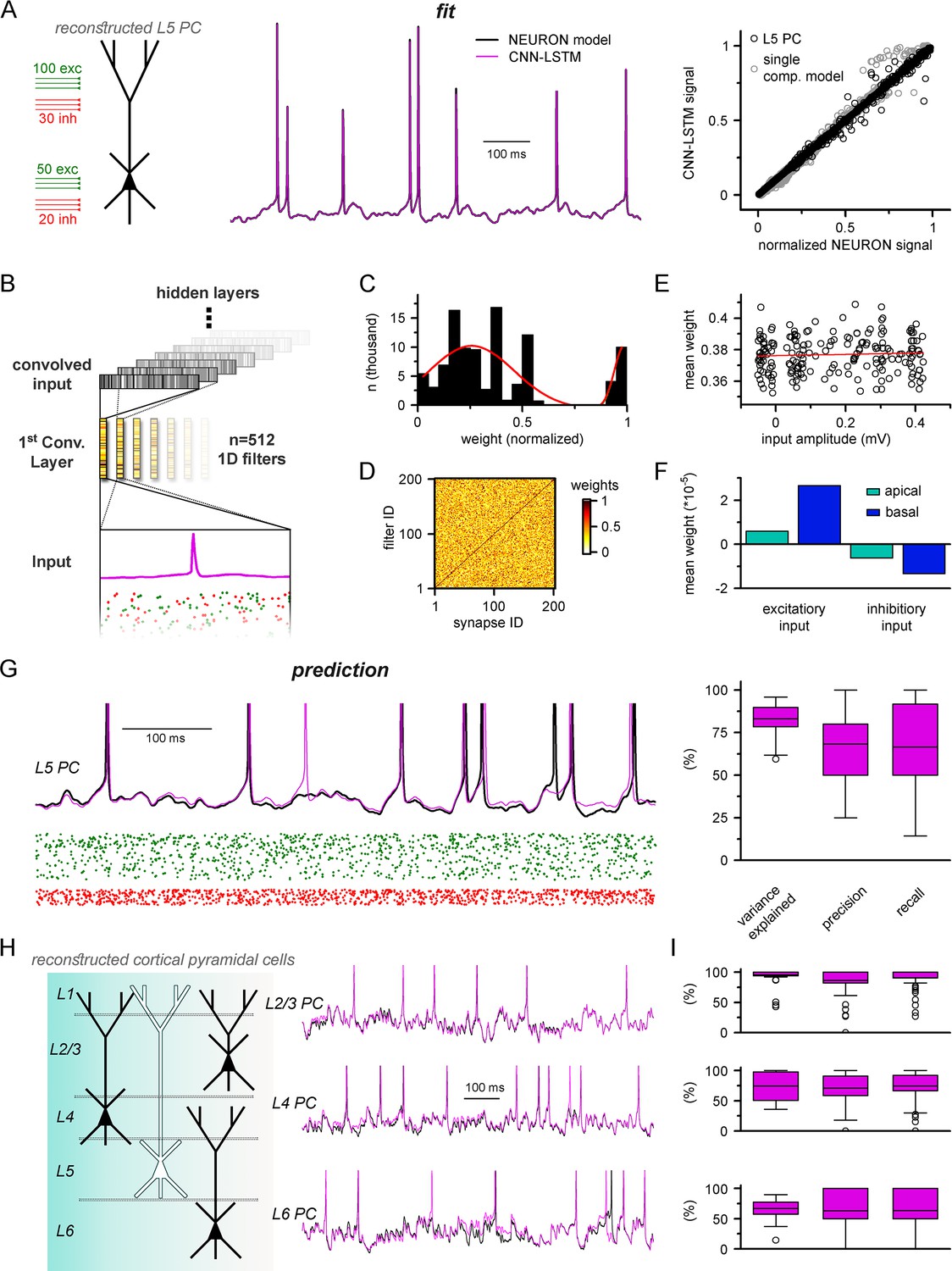
Multicompartmental simulation representation by convolutional neural network-long short-term memory (CNN-LSTM).
(A) CNN-LSTM can accurately predict membrane potential of a multicompartmental neuron upon distributed synaptic stimulation. Representative figure depicts the placement of synaptic inputs (150 excitatory inputs: 100 inputs on apical, oblique, and tuft dendrites and 50 inputs on the basal dendrite, randomly distributed; and 50 inhibitory inputs: 30 inputs on apical, oblique, and tuft dendrites and 20 inputs on the basal dendrite, randomly distributed) of a reconstructed level 5 (L5) pyramidal cell (PC) (left). Point-by-point forecasting of L5 PC membrane potential by a CNN-LSTM superimposed on biophysically detailed NEURON simulation (left). CNN-LSTM prediction accuracy of multicompartmental membrane dynamics is comparable to single-compartmental simulations (right, L5 PC in black, single-compartmental simulation of Figure 1D in gray, n = 45,000 and 50,000, respectively). (B) Convolutional filter information was gathered from the first convolutional layer (middle, color scale depicts the different weights of the filter), which directly processes the input (membrane potential in magenta, excitatory and inhibitory synapse onsets in green and red, respectively), providing convolved inputs to upper layers (gray bars, showing the transformed 1D outputs). (C) Distribution of filter weights from 512 convolutional units (n = 102,400) with double Gaussian fit (red). (D) Filter weight is independent of the somatic amplitude of the input (circles are averages from 512 filters, n = 200, linear fit in red). (E) Each synapse has a dedicated convolutional unit, shown by plotting the filter weights of the 200 most specific units against 200 synapses. Notice the dark diagonal illustrating high filter weights. (F) Excitatory and inhibitory synapse information is convolved by filters with opposing weights (n = 51,200, 25,600, 15,360, and 10,240 for apical excitatory, basal excitatory, apical inhibitory, and basal inhibitory synapses, respectively). (G) Representative continuous prediction of L5 PC membrane dynamics by CNN-LSTM (magenta) compared to NEURON simulation (black) upon synaptic stimulation (left, excitatory input in green, inhibitory input in red). Spike timing is measured on subthreshold traces (right, n = 50 for variance explained, precision and recall). (H) Artificial neural networks (ANNs) constrained on cortical layer 2/3 (top), layer 4 (middle), and layer 6 (bottom) PCs selected from the Allen Institute model database.
Figure 5—figure supplement 1
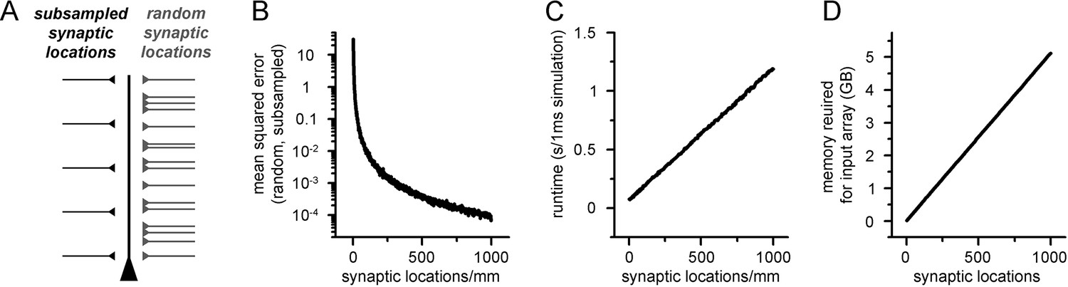
Increased spatial discretization causes reduced errors at the cost of computational overhead.
(A) Methodological illustration of a ball and stick model supplemented with synaptic locations placed at different locations. First, synapses were randomly placed along the dendritic tree (right side, light gray) and the somatic voltage response was recorded. Next, the number of synaptic locations was restricted to a low amount of evenly placed locations, and the previously randomly placed synapses were assigned to the nearest location. The resulting voltage trace was compared to the first arrangement. (B) Mean squared error of voltage traces recorded from models with randomly placed and spatially subsampled synaptic locations as a function of the number of evenly placed synaptic locations. (C) Simulation runtime of artificial neural networks (ANNs) with different input matrix dimensions (number of columns correspond to the number of synaptic locations). (D) Memory requirements of 5000 input matrices with different dimensions.
Figure 5—figure supplement 2
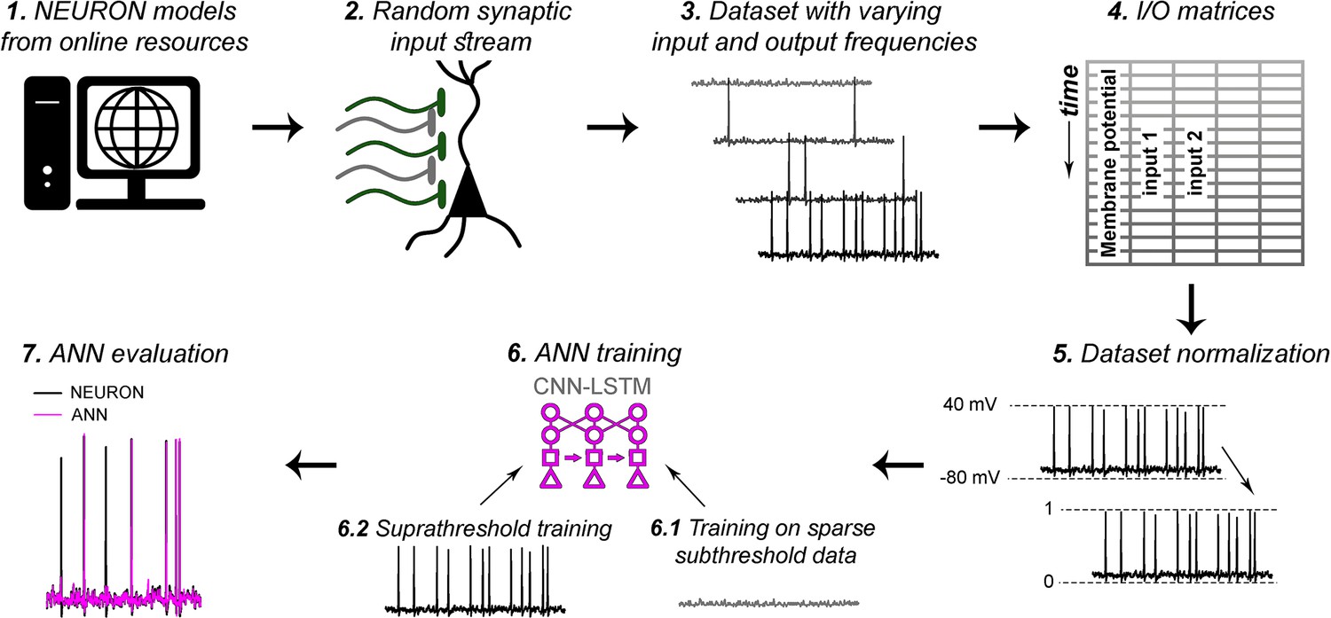
Artificial neural network (ANN) fitting workflow.
As detailed in the ‘Methods’ section, (1) NEURON models were acquired from publicly available, well-curated databases. (2) Synaptic input stream was established at varying number of synaptic locations (200 synaptic locations on level 5 [L5] pyramidal cell [PC] in Figure 5). (3) Voltage traces with varying input frequencies were recorded. (4) Input/output matrices were created from synaptic activations and corresponding voltage recordings. (5) Datasets were normalized to better suit ANN fitting algorithms. Different normalizations were used for different models, based on trial and error (‘Methods’). (6) ANN training consisted of two consecutive steps. First (6.1), ANNs were supplemented with input matrices corresponding to low input frequency recordings, to obtain proper fitting of isolated inputs, and to learn resting membrane potential. Next (6.2), the resulting ANNs received input matrices with higher input frequencies, to learn action potential dynamics, and the spatiotemporal dynamics of distinct synaptic locations. (7) ANNs were evaluated, and further bias terms were established for long-term prediction stability.
Figure 5—figure supplement 3
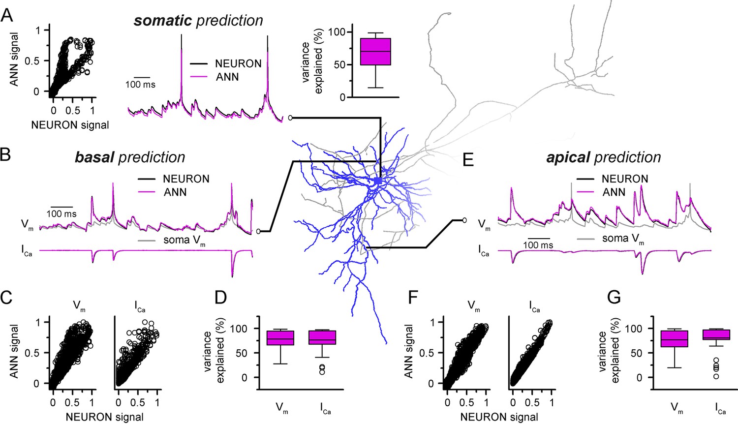
Convolutional neural network-long short-term memory (CNN-LSTM) predictions of dendritic voltage and current fluctuations of a level 2/3 (L2/3) pyramidal cell (PC).
Morphology and biophysical features were obtained from the Cell Types Database of the Allen Institute for Brain Science. (A) Artificial neural network (ANN) signal generated through a point-by-point fit, plotted against NEURON ground truth signal of somatic voltage (left). Representative somatic voltage predictions (magenta) and ground truth NEURON signal (black) in the middle, quantification of explained variance on the right. (B) Representative prediction of membrane voltage (top) and calcium current (bottom) fluctutation at a basal dendritic location. CNN-LSTM predictions in magenta, NEURON signal in black. (C) Basal fit accuracy of CNN-LSTM plotted against NEURON signal. Dendritic membrane voltage on the left, calcium current on the right. (D) Variance explained by CNN-LSTM predictions of basal membrane voltage (left) and calcium currents (right). (E) Representative voltage (top) and calcium current (bottom) fluctuations at an apical dendritic location, quantification of fit accuracy and explained variance in panels (F) and (G) similar as in panels (C) and (D).
Figure 6 with 1 supplement
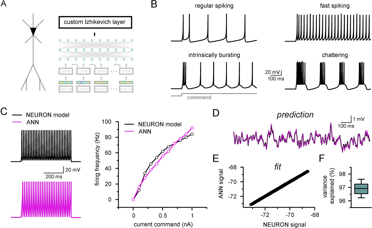
Firing pattern representation with custom artificial neural network (ANN) layer.
(A) Representative figure depicting the custom ANN layer (termed custom Izhikevich layer) placed on the output of the fully connected layers of the convolutional neural network-long short-term memory (CNN-LSTM). This layer represents the final signal integration step, analogous to the soma of biological neurons. (B) Four firing patterns with different activity dynamics, produced by the custom ANN layer. (C) Firing pattern of a NEURON model (black, top) and the constrained ANN counterpart (magenta, bottom). The ANN model accurately reproduced the input–output relationship of the NEURON model. (D) Continuous subthreshold membrane potential fluctuations of the NEURON model (black trace) and faithfully captured by the custom ANN layer (magenta trace). (E) Relationship of membrane potential values predicted step-by-step by the ANN layer compared to the ground truth NEURON model. (F) The custom ANN layer continuous predictions explain the majority of the variance occurring in voltage signals produces by the NEURON simulation.
Figure 6—figure supplement 1
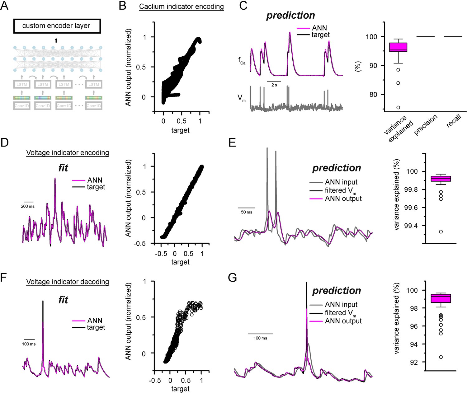
Custom ANN layers for encoding and decoding popular indicators neuronal activity.
(A) Depiction of custom artificial neural network (ANN) layers placed on top of the convolutional neural network-long short-term memory (CNN-LSTM) architecture. (B) Fitting results of the ANN plotted against ground truth signal. (C) Representative simulated calcium indicator traces of ANN predictions (magenta) and NEURON ground truth (black) and the corresponding membrane potential (gray, bottom). Quantification of explained variance, precision, and recall on the right. (D) Encoder ANN fit of voltage indicator signal (ANN, purple; target trace, black), representative trace on the left, fitted values plotted against target signal on the right. (E) Continuous ANN predictions (magenta) are well correlated with target signal (black). Input voltage trace in gray, explained variance quantification on the right. (F) Decoder ANN fit of voltage indicator signal (ANN, purple; target trace, black), representative trace on the left, fitted values plotted against target signal on the right. (G) Continuous ANN predictions (magenta) are in good agreement with target signal (black). Input voltage indicator signal in gray, explained variance quantification on the right.
Figure 7
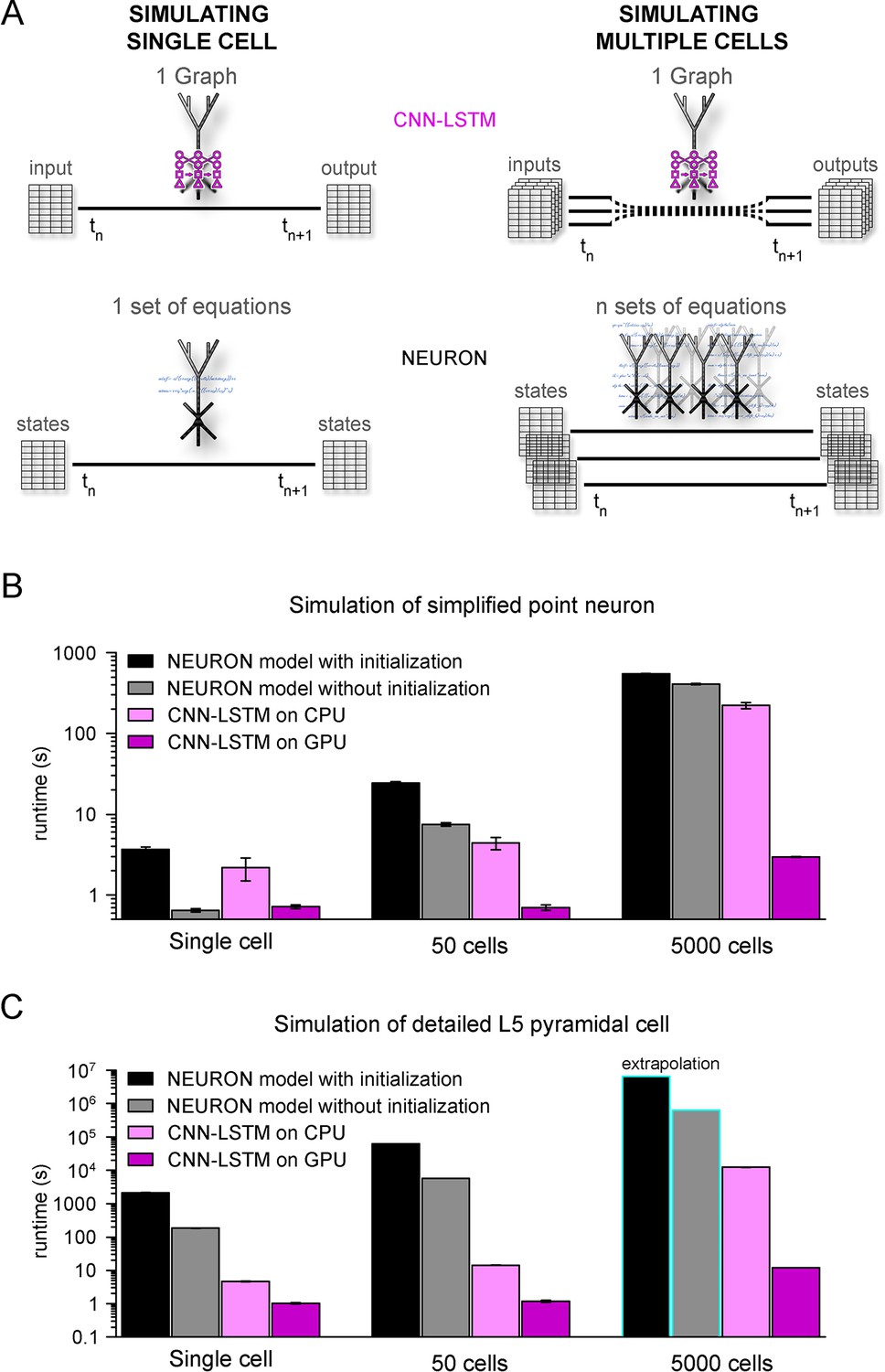
Orders of magnitude faster simulation times with convolutional neural network-long short-term memory (CNN-LSTM).
(A) An illustration demonstrating that CNN-LSTMs (top, magenta) handle both single-cell (left) and multiple-cell (right) simulations with a single graph, while the set of equations to solve increases linearly for NEURON simulations (bottom, black). (B) 100 ms simulation runtimes of 1-, 50-, and 5000-point neurons on four different resources. Bar graphs represent the average of five simulations. (C) Same as in panel (B), but for level 5 (L5) pyramidal cell(PC) simulations. Teal borders represent extrapolated datapoints.
Figure 8

Efficient parameter-space mapping with convolutional neural network-long short-term memory (CNN-LSTM) reveals a joint effect of recurrent connectivity and E/I balance on network stability and efficacy in Rett syndrome.
(A) 150 CNN-LSTM models of level 5 (L5) pyramidal cells (PCs) were simulated in a recurrent microcircuit. (B) The experimental setup consisted of a stable baseline condition for 100 ms, a thalamocortical input at t = 100 ms, and network response, monitored for 150 ms. Example trace from the first simulated CNN-LSTM L5 PC on top, raster plot of 150 L5 PCs in the middle, number of firing cells with 5 ms binning for the same raster plot in the bottom. Time is aligned to the stimulus onset (t = 0, black arrowhead). (C) Simulation runtime for single simulation (left, network of 150 cells simulated for 250 ms) and parameter space mapping (right, 150 cells simulated for 250 ms, 2500 times, for generating B). Teal border represents data extrapolation.
Figure 9 with 1 supplement
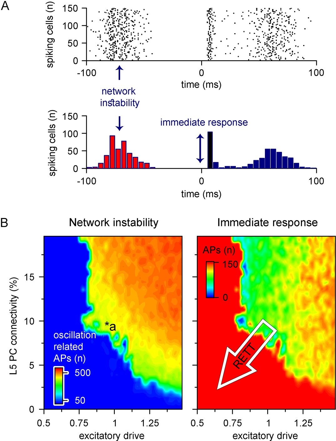
Recurrent connectivity and excitatory drive jointly define network stability in a reduced level 5 (L5) cortical network.
(A) Two independent parameters were quantified: network instability (number of cells firing before the stimulus) and immediate response (number of cells firing within 10 ms of the stimulus onset). The example simulation depicts highly unstable network conditions. (B) Network instability (left) and immediate response (right) as a function of altered L5 pyramidal cell (PC) connectivity and excitatory drive. *a indicates network parameters used for generating panel (A). The white arrow in the right panel denotes circuit alterations observed in Rett syndrome. Namely, 5% recurrent connectivity between L5 PCs instead of 10% in control conditions and reduced excitatory drive.
Figure 9—figure supplement 1

Microcircuit stability and efficacy is robust to changes in inhibitory drive.
Network parameters were quantified as shown in Figure 8A. Recurrent connectivity constrains network stability (9.14 ± 2.21 vs. 320.78 ± 237.66 action potentials [APs], n = 1740 vs. 760 for below 9% connectivity and connectivity between 9–15%, respectively, p=2.2 * 10–219, two-sample t-test), while inhibitory inputs have a negligible effect (133.62 ± 29.32 vs. 131.72 ± 32.32 APs upon thalamocortical stimulus for inhibitory input scaling of 1 and 0.5, respectively, n = 50 each, p=0.76, t(98) = 0.31, two-sample t-test).
Additional files
Download links
A two-part list of links to download the article, or parts of the article, in various formats.
Downloads (link to download the article as PDF)
Open citations (links to open the citations from this article in various online reference manager services)
Cite this article (links to download the citations from this article in formats compatible with various reference manager tools)
Ultrafast simulation of large-scale neocortical microcircuitry with biophysically realistic neurons
eLife 11:e79535.
https://doi.org/10.7554/eLife.79535


