Figures and data in Emergence of time persistence in a data-driven neural network model

Figures
Tables
Additional files

16 figures, 4 tables and 1 additional file

Figures

Figure 1

Download asset Open asset

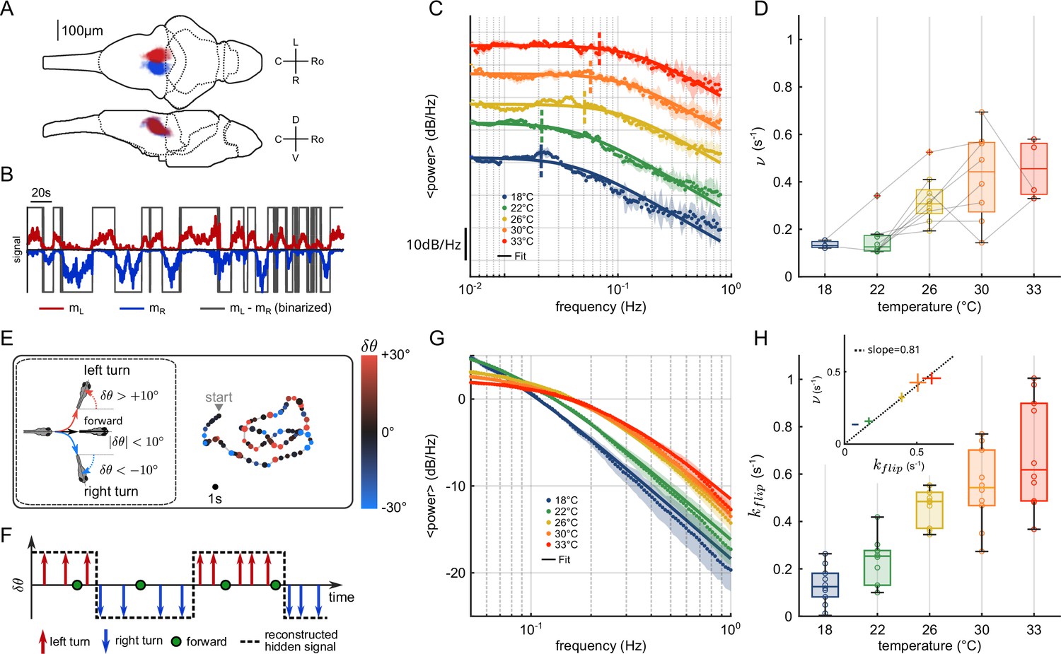
Temperature dependence of anterior rhombencephalic turning region (ARTR) dynamics and turn direction persistence.

(A) Morphological organization of the ARTR showing all identified neurons from 13 fish recorded with light-sheet calcium imaging. (B) Example of ARTR binarized signal sign ( $m_{L} - m_{R}$ ) (gray) along with the left ( $m_{L}$ , red) and right ( $m_{R}$ , blue) mean activities. (C) Averaged power spectra of the ARTR binarized signals for the five tested temperatures. The dotted vertical lines indicate the signal switching frequencies $ν$ as extracted from the Lorentzian fit (solid lines). (D) Temperature dependence of $ν$ . The lines join data points obtained with the same larva. (E) Swimming patterns in zebrafish larvae. Swim bouts are categorized into forward and turn bouts based on the amplitude of the heading reorientation. Example trajectory: each dot corresponds to a swim bout; the color encodes the reorientation angle. (F) The bouts are discretized as left/forward/right bouts. The continuous binary signal represents the putative orientational state governing the chaining of the turn bouts. (G) Power spectra of the discretized orientational signal averaged over all animals for each temperature (dots). Each spectrum is fitted by a Lorentzian function (solid lines) from which we extract the switching rate $k_{f l i p}$ . (H) Temperature dependence of $k_{f l i p}$ . Inset: relationship between $k_{f l i p}$ (behavioral) and $ν$ (neuronal) switching frequencies. Bar sizes represent SEM, and the dashed line is the linear fit.

Figure 2

Download asset Open asset

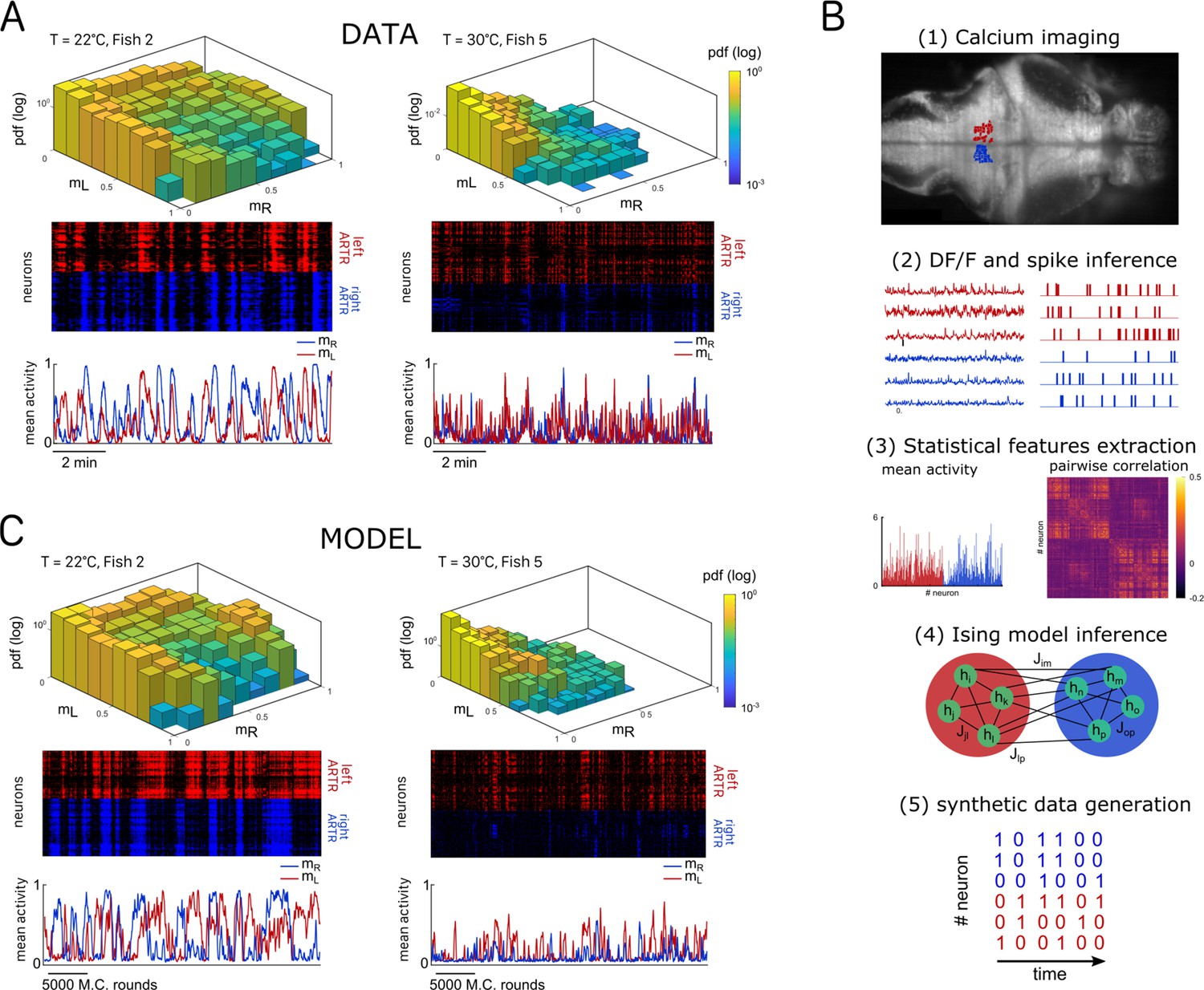
Ising models reproduce characteristic features of the recorded activity.

(A) (Top) Probability densities $P (m_{L}, m_{R})$ , see Equation 2, of the activity state of the circuit (obtained from the spiking inference of the calcium data), in logarithmic scale, and for two different fish and water temperatures T = 20 and T = 30°C; Color encodes z-axis (same color bar for both). (Middle) 10-min-long raster plots of the activities of the left (red) and right (blue) subregions of the anterior rhombencephalic turning region (ARTR). (Bottom) Corresponding time traces of the mean activities $m_{L}$ and $m_{R}$ . (B) Processing pipeline for the inference of the Ising model. We first extract from the recorded fluorescence signals approximate spike trains using a Bayesian deconvolution algorithm (BSD). The activity of each neuron is then ‘0’ or ‘1.’ We then compute the mean activity and the pairwise covariance of the data, from which we infer the parameters $h_{i}$ and $J_{i j}$ of the Ising model. Finally, we can generate raster plot of activity using Monte Carlo sampling. (C) Same as (A) for the two corresponding inferred Ising models. The raster plots correspond to Monte Carlo-sampled activity, showing slow alternance between periods of high activity in the L/R regions. Here we show only two examples of a qualitative experimental vs. synthetic signals comparison. We provide in the supplementary materials the same comparison for every recording.

Figure 3

Download asset Open asset

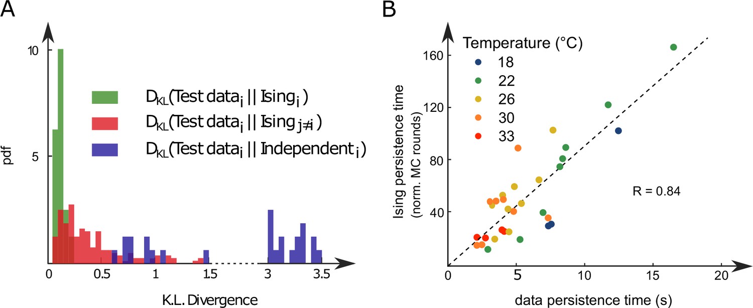
Comparison of model distributions and persistence times across fish and water temperatures.

(A) Distribution of the Kullback–Leibler divergences between test datasets and their corresponding Ising models (green), between test datasets and Ising models trained on different datasets (red) and between test datasets and their corresponding independent models that assume no connections between neurons (dark blue). Note that each dataset is divided in a training set corresponding to 75% of the time bins chosen randomly and a test set comprising the remaining 25%. (B) Average persistence times in simulations vs. experiments. Each dot refers to one fish at one water temperature; colors encode temperature.

Figure 4

Download asset Open asset

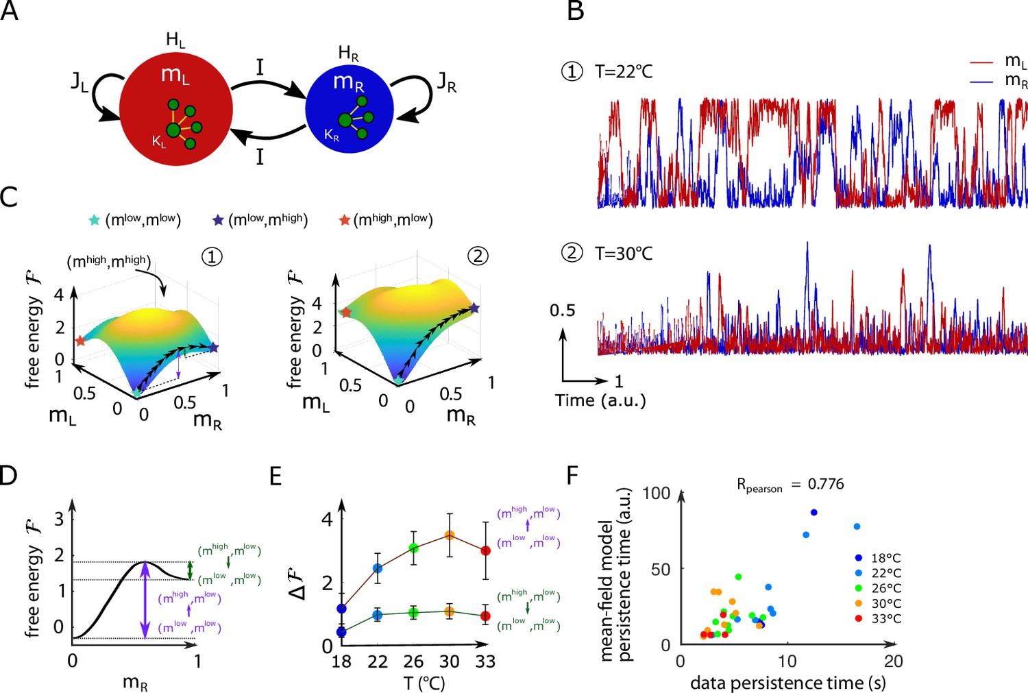
Mean-field approximation of the inferred Ising model.

(A) Schematic view of the mean-field Ising model. (B) Examples of simulated $m_{L}$ and $m_{R}$ signals of the mean-field dynamical equations for two sets of parameters that correspond to fish ID #5 at two water temperatures (22°C and 30°C), see Appendix 2—table 2. (C) Free-energy landscapes in the ( $m_{L}$ , $m_{R}$ ) plane computed with the mean-field model. These data correspond to the same sets of parameters as in panel (B). Colored circles denote metastable states, and the line of black arrows indicates the optimal path between $(m^{l o w}, m^{l o w})$ and $(m^{l o w}$ , $m^{h i g h})$ states. (D) Schematic view of the free energy along the $m_{R}$ axes. The arrows denote the energy barriers $Δ$ $ℱ$ associated with the various transitions. The dark green arrow denotes $Δ F ((m^{h i g h}, m^{l o w}) \to (m^{l o w}, m^{l o w}))$ ; the purple arrow denotes $Δ F ((m^{l o w}, m^{l o w}) \to (m^{h i g h}, m^{l o w}))$ . (E) Values of the free-energy barriers as a function of temperature. Error bars are standard error of the mean (32 recordings, n = 13 fish at 5 different water temperatures). (F) Persistence time of the mean-field anterior rhombencephalic turning region (ARTR) model for all fish and runs at different experimental temperatures. Each dot refers to one fish at one temperature; colors encode temperature.

Figure 5

Download asset Open asset

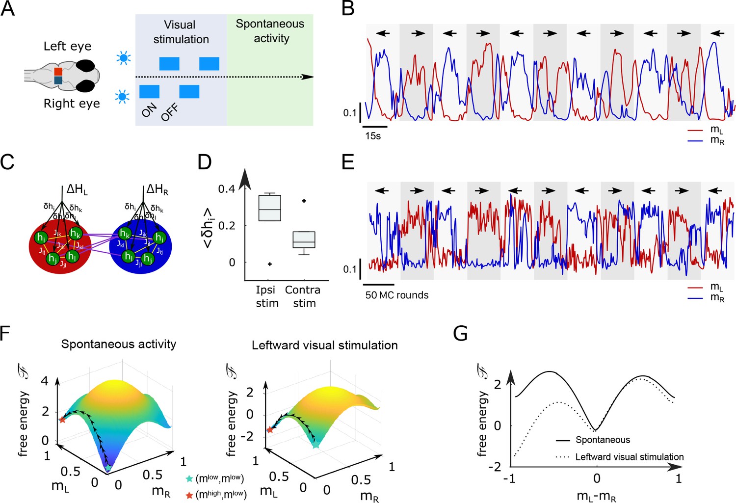
Modified Ising model captures the behavior of anterior rhombencephalic turning region (ARTR) under visual stimulation.

(A) Scheme of the stimulation protocol. The left and right eyes are stimulated alternatively for periods of 15–30 s, after which a period of spontaneous (no stimulus) activity is acquired. (B) Example of the ARTR activity signals under alternated left–right visual stimulation. The small arrows indicate the direction of the stimulus. (C) Sketch of the modified Ising model, with additional biases $δ h_{i}$ to account for the local visual inputs. (D) Values of the additional biases averaged over the ipsilateral and contralateral (with respect to the illuminated eye) neural populations. n = 6 fish. (E) Monte Carlo activity traces generated with the modified Ising model. (F) Free-energy landscapes computed with the mean-field theory during spontaneous (left panel) and stimulated (right panel) activity for an example fish. (G) Free-energy along the optimal path as a function of $m_{L} - m_{R}$ during spontaneous (plain line) and stimulated (dotted line) activity. The model is the same as in panel (F).

Appendix 2—figure 1

Download asset Open asset

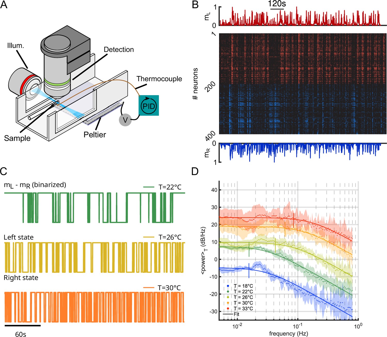
Temperature dependence of the anterior rhombencephalic turning region (ARTR) activity.

(A) Schematic of the experimental setup used to perform brain-wide calcium imaging of a zebrafish larva at controlled water temperature. (B) Raster plot of the ARTR spontaneous dynamics showing alternating right/left activation. The top and bottom traces are the ARTR average signal of the left and right subcircuits. (C) Example ARTR sign( $m_{L} - m_{R}$ ) binarized signals measured at three different temperatures (same larva). (D) Averaged power spectrum of the ARTR signals $m_{R} - m_{L}$ for the five tested temperatures. Lorentzian fits are shown as solid lines.

Appendix 2—figure 2

Download asset Open asset

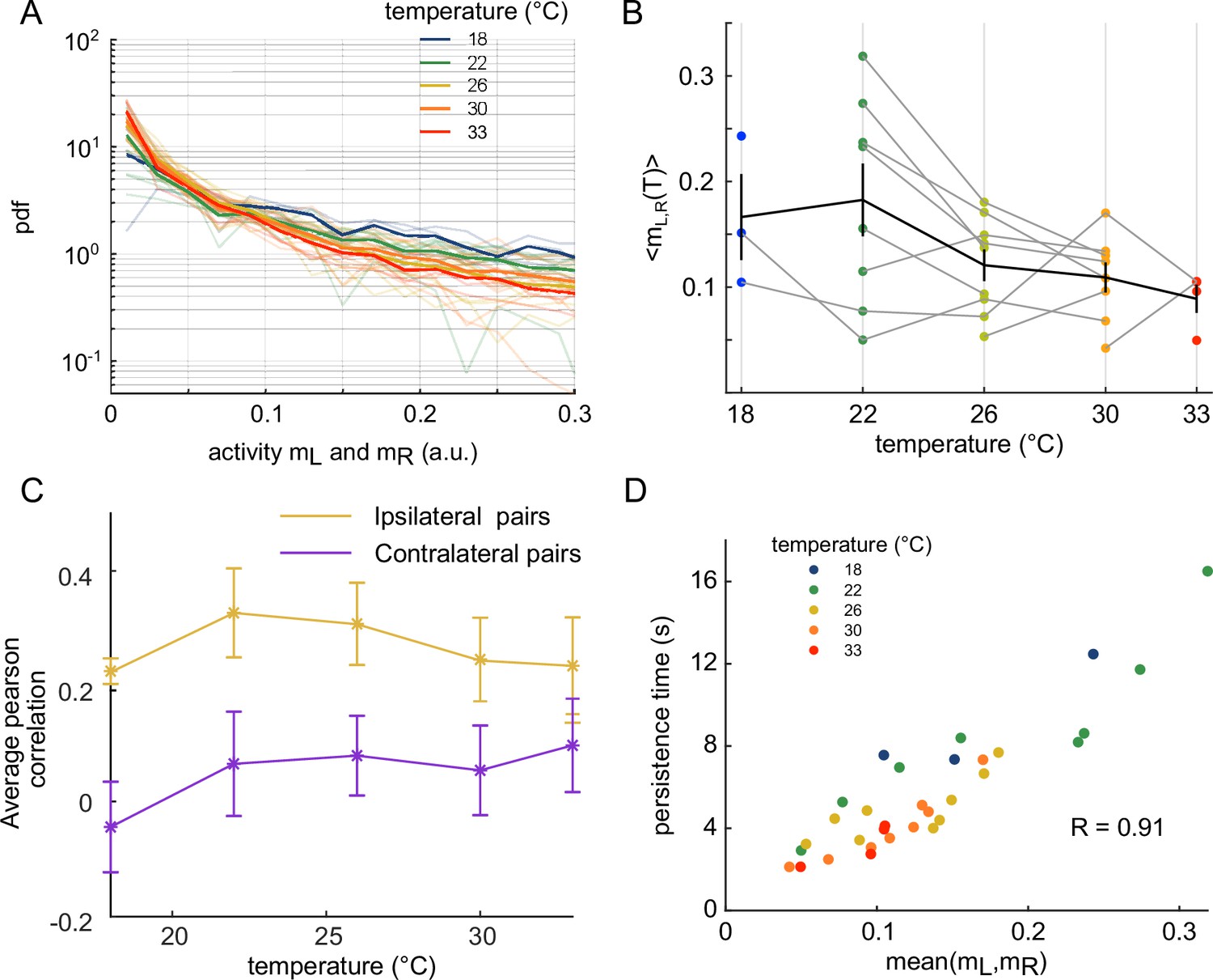
Effect of temperature on the anterior rhombencephalic turning region (ARTR) time persistence and activity.

(A) Pdf of activities of both sides of the ARTR. Color encodes temperature. (B) Temperature-averaged mean activity of ARTR left and right neuronal subpopulations. Error bars are standard error of the mean. (C) Temperature-averaged Pearson correlation for left/right ispilateral pairs (yellow line) or for contralateral pairs of neurons (purple line). Error bars are standard deviations (32 recordings), n = 13 fish at 5 different water temperatures. (D) ARTR persistence time vs. mean activity; note the quasi-linear dependence of these quantities ( $R = 0.91$ ). Each dot is the mean persistence time computed for one fish at one temperature; colors encode temperature.

Appendix 2—figure 3

Download asset Open asset

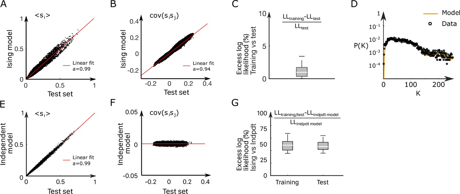
Inference of the anterior rhombencephalic turning region (ARTR) Ising model.

(**A, B**) Comparison between the mean activities (A) and pairwise correlations (B) computed from experimental test data and from synthetic (Ising model-generated) data (32 recordings, n = 13 fish). Ising models were trained on a distinct subset of the experimental data. (C) Relative variation of the log–likelihoods of the Ising models between training and test data, showing the absence of overfitting. (D) Probability that $K$ of the $N$ neurons in the ARTR are simultaneously active in the data (black dots) and in the model (yellow line) configurations. (**E, F**) In order to demonstrate the need for effective connections in our model, we generated synthetic data with independent models of the training dataset. Here, we compare the mean activity (E) and the pairwise covariance (F) computed on the experimental test dataset and using independent models. (G) Excess log likelihood of the Ising models compared to the independent model for training and test data set (see ‘Materials and methods’).

Appendix 2—figure 4

Download asset Open asset

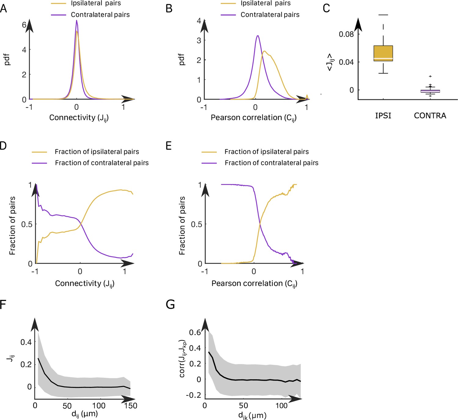
Correlation structure within the anterior rhombencephalic turning region (ARTR) and properties of the inferred couplings.

(A) Probability density function of the functional connectivity for the ipsilateral (gold line) and the contralateral (purple line) couplings. These pdf were obtained by averaging across all animals. (B) Probability density function of the functional Pearson correlation for the ipsilateral (gold line) and the contralateral (purple line) couplings. (C) Box plot across experiments of the average value of the ipsilateral and contralateral couplings. (D) Probability to have an ipsilateral (gold line) or a contralateral (purple line) pair of neuron given its effective connectivity. For a given range of the effective connectivity, we compute the number of ipsilateral and contralateral pairs of neurons. (E) Probability to have an ipsilateral (gold line) or a contralateral (purple line) pair of neuron given its Pearson correlation. (F) Functional connectivity $J_{i j}$ as a function of the distance between neurons $i, j$ . (G) Correlation between the couplings $J_{i j}$ and $J_{k p}$ , between one neuron $i$ and one neuron $k$ as a function of their distance $d_{i k}$ for every possible pair $(i, k)$ .

Appendix 2—figure 5

Download asset Open asset

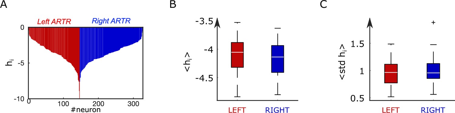
Distribution of biases in the inferred anterior rhombencephalic turning region (ARTR) Ising model.

(A) Bias parameter distribution for an example fish. (B) Box plot across experiments of the average value of the biases for the left and right subpopulations of the ARTR. (C) Box plot across animals of the standard deviation of the biases for the left and right subpopulations of the ARTR.

Appendix 2—figure 6

Download asset Open asset

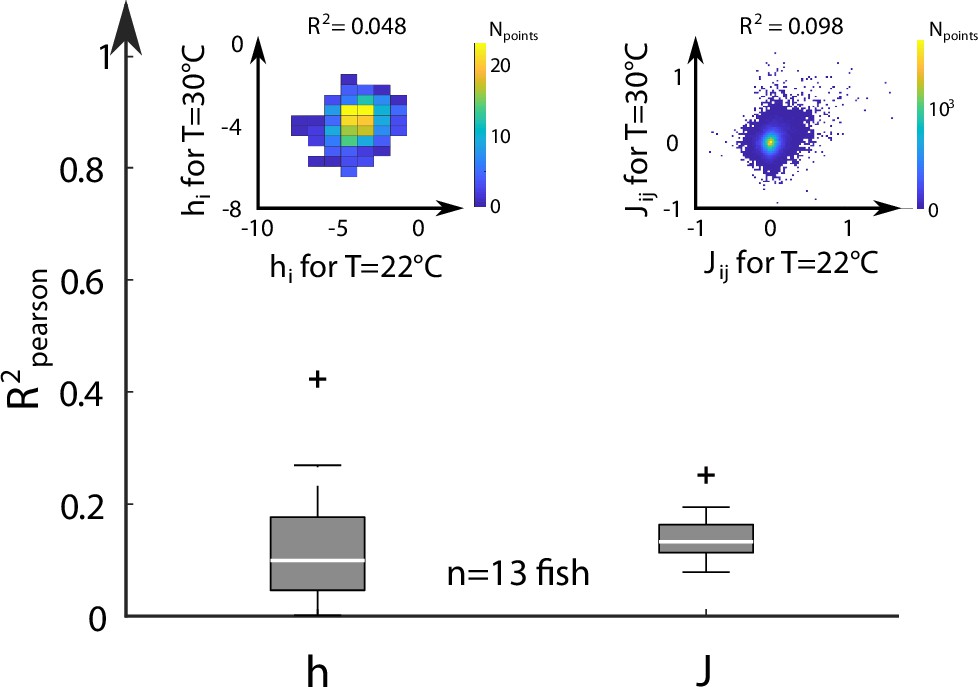
Correlation of Ising parameters at different temperatures.

For each fish (n = 13), we extract from the scatter plots of the coupling $J_{i j}$ and bias h_i inferred from activity recordings at two different temperatures, the Pearson correlation coefficients $R_{p e a r s o n}$ . The distribution of $R_{p e a r s o n}^{2}$ values are shown for all fish and pairs of temperature. Inset: Example scatter plots of the inferred biases h_i (left) and effective couplings $J_{i j}$ (right) for the same fish at two different temperature T = 22 and T = 30°C.

Appendix 2—figure 7

Download asset Open asset

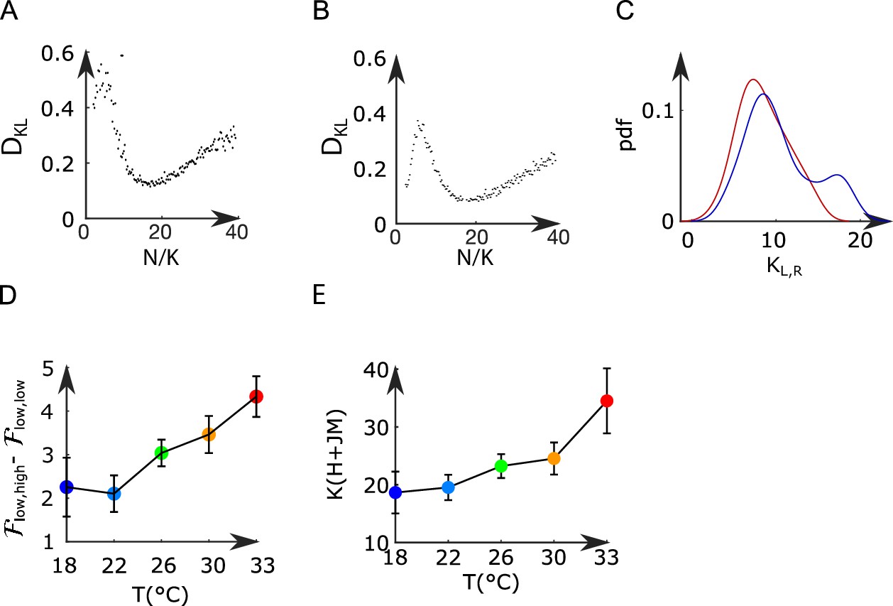
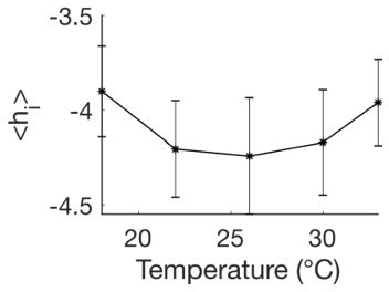
Mean-field model of the anterior rhombencephalic turning region (ARTR).

(**A, B**) Kullback–Leibler divergence between the experimental and the Langevin distributions as a function of $N / K$ , where $N$ is the total number of neurons of the left or right subpopulation, and $K$ is the effective extent of neuronal interaction (see ‘Materials and methods’) for two datasets. (C) Probability density function of $K_{R}$ (blue line) and $K_{L}$ (red line) across all recordings. (D) Free-energy difference between stationary sates of the landscape as a function of the temperature (32 recordings, n=13 fish). (E) Average values (for all experiments and regions) of $K (H + J M)$ as a function of the temperature of the water. Error bars are standard error of the mean.

Appendix 2—figure 8

Download asset Open asset

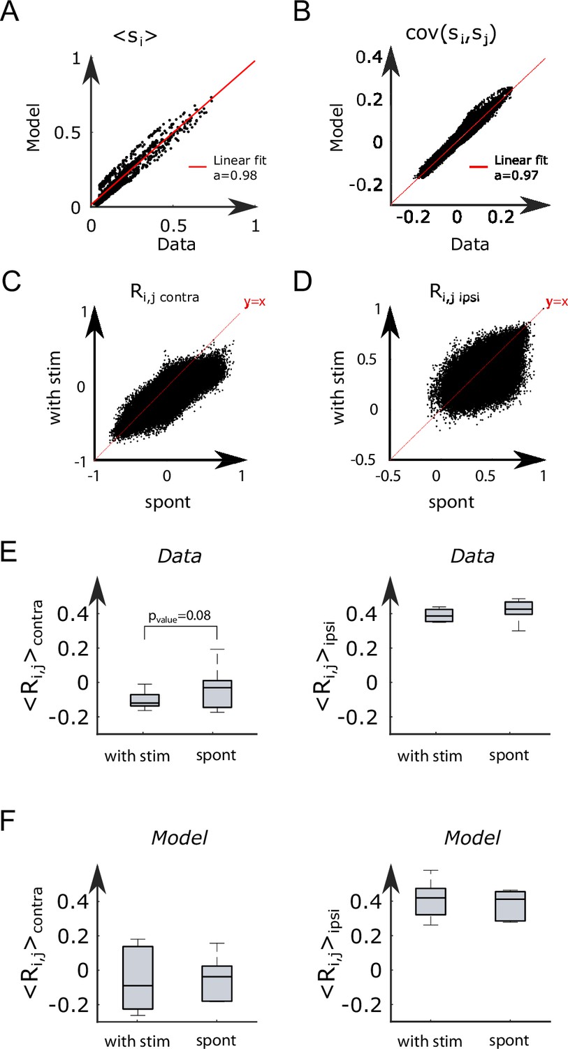
A modified Ising model explains visually driven properties of the anterior rhombencephalic turning region (ARTR).

(**A, B**) To assess the performance of the model for visually driven experiments, we compare the mean activity (A) and the pairwise covariance (B) computed on the spontaneous part of the recordings to synthetic data. (C) Scatter plot of the correlation between contralateral pairs of neurons under visual stimulation vs. spontaneous activity on n = 6 fish. (D) Scatter plot of the correlation between ipsilateral pairs of neurons under visual stimulation vs. spontaneous activity. (E) Average Pearson correlation in the experimental recordings between contralateral (the p-value of a paired sampled t-test is provided) and ipsilateral pairs of cells during stimulated and spontaneous activity (n = 6 fish). (F) Average Pearson correlation in the simulated activity of the ARTR between contralateral and ipsilateral pairs of cells during stimulated and spontaneous activity (n = 6 fish).

Author response image 1

Download asset Open asset

Author response image 2

Download asset Open asset

Author response image 3

Download asset Open asset

Tables

Key resources table

Reagent type (species) or resource	Designation	Source or reference	Identifiers
Strain, strain background (Danio rerio)	Tg(elavl3:H2B-GCaMP6s)	Vladimirov et al., 2014
Strain, strain background (D. rerio)	Tg(elavl3:H2B-GCaMP6f)	Quirin et al., 2016
Software, algorithm	Blind Sparse Deconvolution	Tubiana et al., 2020	BSD
Software, algorithm	Computational Morphometry Toolkit	https://www.nitrc.org/projects/cmtk/	CMTK
Software, algorithm	Adaptive Cluster Expansion	Barton and Cocco, 2013	ACE

Appendix 2—table 1

Datasets properties.

Temperature (°C)	ID	Line	Age (dpf)	$N_{L}$	$N_{R}$	Acquisition rate (Hz)	Duration (s)
18	12	NucFast	6	146	180	5	1200
18	13	NucFast	7	37	96	8	1200
18	14	NucFast	6	179	174	8	1200
22	2	Nuc slow	7	177	212	3	1106
22	3	NucFast	5	152	85	3	1812
22	5	NucFast	5	158	123	5	1500
22	6	NucFast	5	98	134	5	1500
22	7	NucFast	6	122	221	5	1500
22	11	NucFast	6	295	320	5	1200
22	13	NucFast	7	37	96	8	1200
22	14	NucFast	6	179	174	8	1200
26	2	Nuc slow	7	177	212	3	1812
26	3	NucFast	5	152	85	3	1812
26	4	NucFast	5	110	76	3	1812
26	5	NucFast	5	158	123	5	1500
26	6	NucFast	5	98	134	5	1500
26	7	NucFast	6	122	221	5	1500
26	11	NucFast	6	295	320	5	1200
26	13	NucFast	7	37	96	8	1200
26	14	NucFast	6	179	174	8	1200
30	2	Nuc slow	7	177	212	3	1812
30	4	NucFast	5	110	76	3	1812
30	5	NucFast	5	158	123	5	1500
30	6	NucFast	5	98	134	5	1500
30	7	NucFast	6	122	221	5	1500
30	13	NucFast	7	37	96	8	1200
30	14	NucFast	6	179	174	8	1200
30	15	NucFast	7	202	252	8	1200
33	14	NucFast	6	179	174	8	1200
33	15	NucFast	7	202	252	8	1200
33	16	NucFast	6	127	123	7	1200
33	17	NucFast	5	62	170	10	1200

Appendix 2—table 2

Parameters of mean-field models.

Temperature (°C)	ID	$J_{L}$	$J_{R}$	$I$	$H_{L}$	$H_{R}$	$K_{L}$	$K_{R}$
18	12	7.06	7.23	–0.6	–3.66	–3.63	6.51	8.03
18	13	6.2	7.84	0.6	–3.53	–4.34	3.18	8.27
18	14	7.27	7.24	0.31	–3.88	–3.99	11.04	10.74
22	2	8.2	8.28	0.12	–4.24	–4.23	6.65	7.96
22	3	8.18	7.14	0.55	–4.26	–4.13	9.38	5.24
22	5	7.59	7.01	0.4	–4.03	–3.8	5.56	4.33
22	6	7.13	8.69	1.1	–4.49	–4.64	5.21	7.12
22	7	7.09	7.46	0.43	–3.73	–3.95	6.28	11.39
22	11	7.82	7.59	–0.1	–4.07	–3.91	8.28	8.98
22	13	6.54	7.82	1.45	–4.29	–4.5	7.11	18.46
22	14	7.41	8.03	0.47	–4.28	–4.43	10.91	10.6
26	2	8.37	8.22	–0.49	–4.47	–4.31	9.72	11.64
26	3	8.42	7.49	0.53	–4.56	–4.62	8.26	4.61
26	4	8.63	6.44	0.85	–4.83	–4.79	10.37	7.16
26	5	7.29	7.59	0.48	–3.92	–4.14	9.08	7.06
26	6	7.43	7.86	0.41	–3.99	–4.1	8.59	11.75
26	7	7.55	7.96	0.32	–4.08	–4.22	4.45	8.06
26	11	7.27	7.45	0.37	–3.89	–3.92	10.31	11.18
26	13	6.99	7.3	0.6	–3.99	–3.94	6.37	16.55
26	14	7.91	7.35	0.5	–4.34	–4.16	11.32	11.01
30	2	7.54	7.96	–0.12	–4.54	–4.56	7.02	8.41
30	4	8.36	7.73	0.11	–4.52	–4.18	9.64	6.66
30	5	6.77	6.42	0.66	–3.8	–3.87	9.18	7.15
30	6	7.35	7.38	0.45	–3.91	–3.97	7.53	10.3
30	7	7.43	8.07	0.42	–3.93	–4.38	7.09	12.84
30	13	6.91	7.41	0.73	–4.13	–4.03	5.78	15
30	14	7.51	7.45	0.11	–3.87	–3.89	9.42	9.15
30	15	8.01	8.33	0.58	–4.45	–4.46	13.83	17.26
33	14	6.74	7.02	0.76	–3.8	–3.97	9.32	9.06
33	15	6.99	7.47	–0.02	–3.68	–3.91	14.85	18.52
33	16	7.53	8.25	–0.11	–4.16	–4.43	14.43	13.97
33	17	6.66	7.36	0.45	–3.69	–3.89	11.92	32.69

Appendix 2—table 3

Parameters of mean-field models.

ID	$J_{L}$	$J_{R}$	$I$	$H_{L}$	$H_{R}$	$K_{L}$	$K_{R}$
1	7.54	7.35	–0.67	–3.75	–3.44	5.60	3.43
2	7.10	7.42	0.64	–3.69	–4.02	7.91	12.82
3	7.51	7.92	–0.28	–3.96	–4.08	4.98	3.90
4	8.38	6.25	–0.04	–3.68	–3.18	13.33	4.44
5	8.73	8.24	0.01	–4.38	–4.13	6.11	6.89
6	7.87	7.71	0.51	–4.17	–4.09	16.19	15.52

Additional files

MDAR checklist: https://cdn.elifesciences.org/articles/79541/elife-79541-mdarchecklist1-v2.docx
Download elife-79541-mdarchecklist1-v2.docx

Download links

A two-part list of links to download the article, or parts of the article, in various formats.

Downloads (link to download the article as PDF)

Article PDF

Open citations (links to open the citations from this article in various online reference manager services)

Mendeley

Cite this article (links to download the citations from this article in formats compatible with various reference manager tools)

Sebastien Wolf
Guillaume Le Goc
Georges Debrégeas
Simona Cocco
Rémi Monasson

(2023)

Emergence of time persistence in a data-driven neural network model

eLife 12:e79541.

https://doi.org/10.7554/eLife.79541

Share this article

Cite this article

Temperature dependence of anterior rhombencephalic turning region (ARTR) dynamics and turn direction persistence.

Ising models reproduce characteristic features of the recorded activity.

Comparison of model distributions and persistence times across fish and water temperatures.

Mean-field approximation of the inferred Ising model.

Modified Ising model captures the behavior of anterior rhombencephalic turning region (ARTR) under visual stimulation.

Temperature dependence of the anterior rhombencephalic turning region (ARTR) activity.

Effect of temperature on the anterior rhombencephalic turning region (ARTR) time persistence and activity.

Inference of the anterior rhombencephalic turning region (ARTR) Ising model.

Correlation structure within the anterior rhombencephalic turning region (ARTR) and properties of the inferred couplings.

Distribution of biases in the inferred anterior rhombencephalic turning region (ARTR) Ising model.

Correlation of Ising parameters at different temperatures.

Mean-field model of the anterior rhombencephalic turning region (ARTR).

A modified Ising model explains visually driven properties of the anterior rhombencephalic turning region (ARTR).

Datasets properties.

Parameters of mean-field models.

Parameters of mean-field models.

MDAR checklist

Downloads (link to download the article as PDF)

Open citations (links to open the citations from this article in various online reference manager services)

Cite this article (links to download the citations from this article in formats compatible with various reference manager tools)