Circular and unified analysis in network neuroscience
- Departments of Biomedical Engineering, Computer Science, and Psychology, Vanderbilt University, United States
- Janelia Research Campus, Howard Hughes Medical Institute, United States
Figures
Figure 1
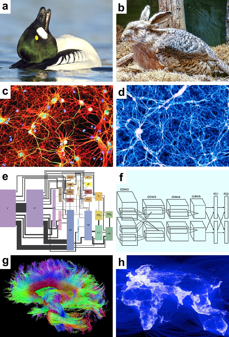
Speculative models.
Speculative hypotheses that rest on apparent similarities between (a) an ambiguous duck-rabbit animal and (b) a skvader, a type of winged hare; (c) networks of neurons and (d) networks of galaxies; (e) a cortical visual system and (f) a convolutional neural network, a machine learning model for classifying images; (g) large-scale brain networks and (h) global friendship networks. Panel (a) is reproduced from Tim Zurowski (Shutterstock). Panel (b) is reproduced from Gösta Knochenhauer. Panel (c) is reproduced from Figure 4.2 of Stangor and Walinga, 2014. Panel (d) is adapted from the Illustris Collaboration (Vogelsberger et al., 2014). Panel (e) is reproduced from Figure 1 of Wallisch and Movshon, 2008. Panel (f) is adapted from Figure 2 of Krizhevsky et al., 2012. Panel (g) is reproduced from the USC Laboratory of NeuroImaging and Athinoula A. Martinos Center for Biomedical Imaging Human Connectome Project Consortium. Panel (h) is reproduced from Paul Butler (Facebook).
© 2017, Tim Zurowski (Shutterstock). Panel (a) is reproduced from Tim Zurowski (Shutterstock). It is not covered by the CC-BY 4.0 license and further reproduction of this panel would need permission from the copyright holder.
© 2015, Gösta Knochenhauer. Panel (b) is reproduced from Gösta Knochenhauer with permission. It is not covered by the CC-BY 4.0 license and further reproduction of this panel would need permission from the copyright holder.
Figure 2
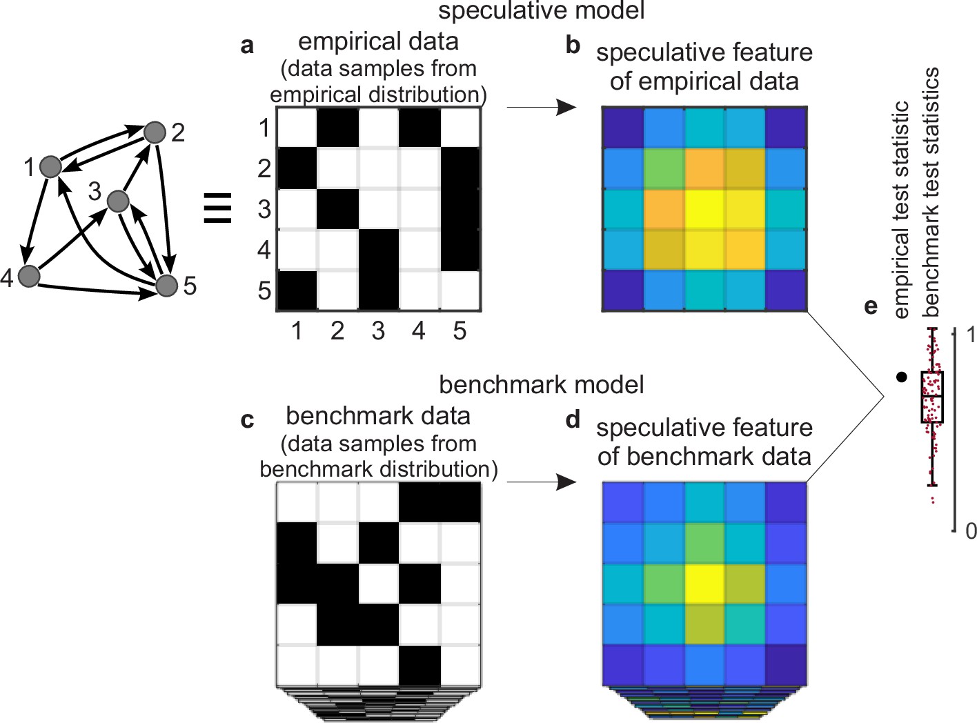
Tests against benchmark models.
(a) An empirical data sample. The diagram (left) shows a network representation of this sample. This example shows only one empirical data sample, but in general there could be many such samples. (b) A speculative feature computed on empirical data. In this example, the feature has the same size as the data, but in general it could have an arbitrary size. Colors denote values of feature elements. (c–d) Corresponding (c) benchmark data samples and (d) speculative features computed on these data. (e) Empirical test statistic (large black dot) and corresponding benchmark test statistics (small red dots). The effect size reflects the deviation of the empirical test statistic from the benchmark test statistic. The uncertainty (confidence) interval and p-value reflect the statistical significance of this deviation. This panel shows a non-significant effect and thus implies that the speculative feature does not transcend the benchmark model of existing knowledge.
Figure 3
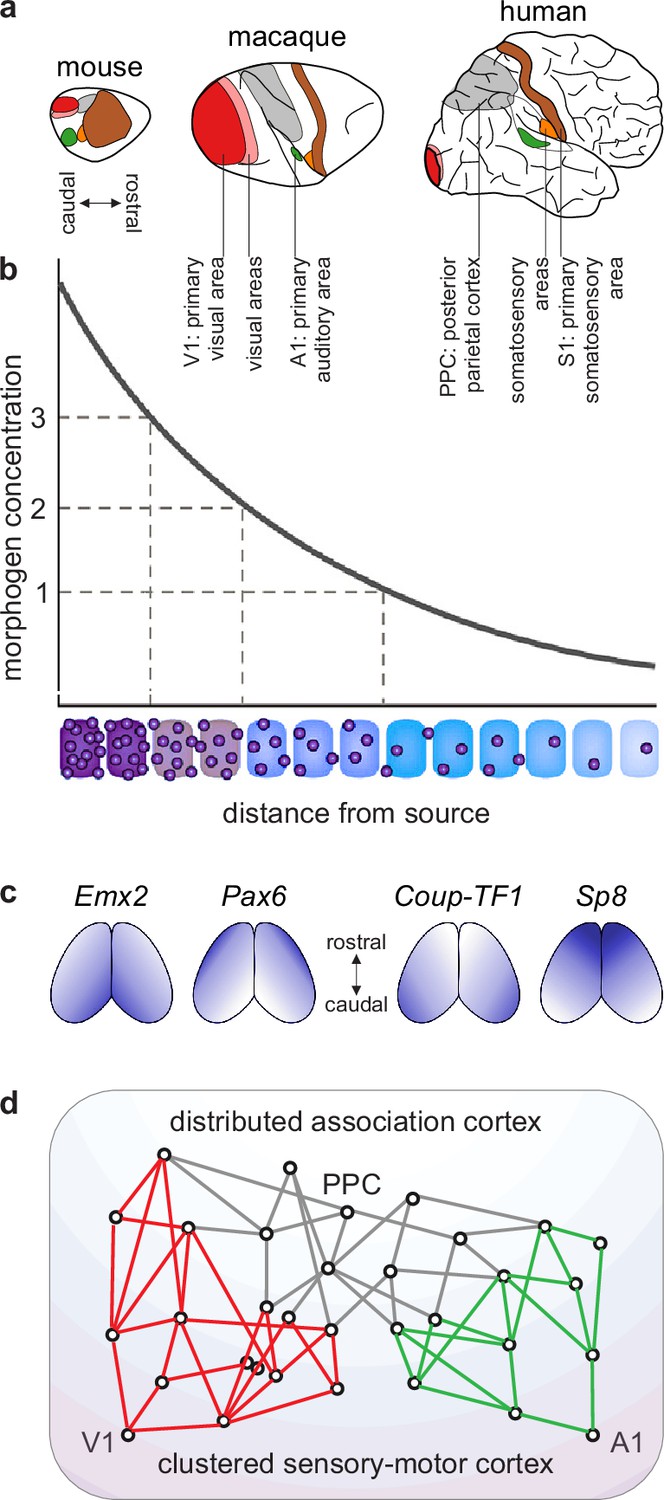
A blueprint of large-scale cortical networks.
(a) Rostrocaudal (nose-to-tail) maps of shared cortical regions in three popular mammalian model organisms. Virtually all mammals have well-delineated primary and other sensory areas, and an ill-delineated posterior parietal association cortex. In addition, most mammals have well-delineated primary and other motor areas (not highlighted in this panel). (b–c) Gradients of cortical development. (b) Spatial gradients of morphogen concentration induce corresponding (c) spatial gradients of transcription-factor and gene expression. Morphogens are signaling molecules that establish spatial concentration gradients through extracellular diffusion from specific sites. Transcription factors (names in italics) are intracellular proteins that establish spatial gradients of gene expression. The discretization of these gradients during development results in the formation of discrete cortical areas and systems (colors in b). (d) A schematized blueprint of a macaque cortical network reflects a gradual transition of a relatively clustered sensory-motor cortex (red and green) into a relatively distributed association cortex (gray). Circles denote cortical regions, while lines denote interregional projections. V1 and A1 denote primary visual and auditory areas, while PPC denotes posterior parietal association cortex. Panel (a) is adapted from Figure 3 of Krubitzer and Prescott, 2018. Panel (b) is adapted from Figure 1.3b of Grove and Monuki, 2020. Panel (c) is adapted from Figure 2 of Borello and Pierani, 2010. Panel (d) is adapted from Figure 2d of Mesulam, 1998.
Figure 4
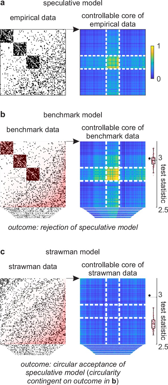
Example analysis.
(a) Left: A toy cortical network. Right: A matrix that reflects the controllability of specific network states (a one-rank approximation of the controllability Gramian [Brunton and Kutz, 2019]). Dashed lines delineate the controllable core. The test statistic is the logarithm of the sum of all matrix elements within this core. (b) Left: Data samples from a benchmark-model distribution. The benchmark model includes empirical network modules and node connectivity (red overlays). Right: Controllable cores in benchmark-model data. Rightmost: Empirical (large black dot) and benchmark test statistics (small red dots). (c) Left: Data samples from a strawman model distribution. The strawman model includes node connectivity but not empirical network modules (red overlay). Right: Controllable cores in strawman-model data. Rightmost: Empirical test statistic (large black dot) and strawman test statistics (small red dots).
Figure 5
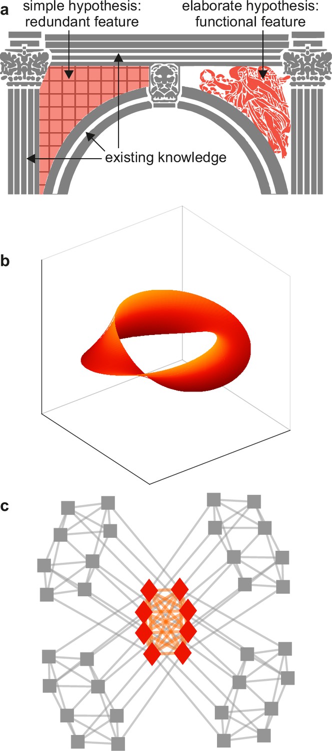
Example spandrels.
(a) Spandrels in architecture denote triangular spaces of building arches (left, orange). Existing knowledge (gray) may explain these spaces as byproducts, but their intricate structure (right, orange) may suggest that they have important function. (b) An illustrative depiction of a “manifold” representation of neuronal population activity (orange). Axes denote directions of neuronal population activity in low-dimensional space. The intricate structure and predictive success of this feature may suggest that it plays an important role in neural function. The difficulty of testing this importance against existing knowledge (not shown) can make this importance speculative. (c) An illustrative depiction of a cortical core (orange). The intricate structure of this feature may suggest that it plays an important role in neural function. The relative ease of testing this importance against existing knowledge (gray) makes it possible to show that this feature is ultimately redundant. Panels (a) and (c) are adapted from (respectively) Figure 2b and Figure 1a of Rubinov, 2016.
Figure 6
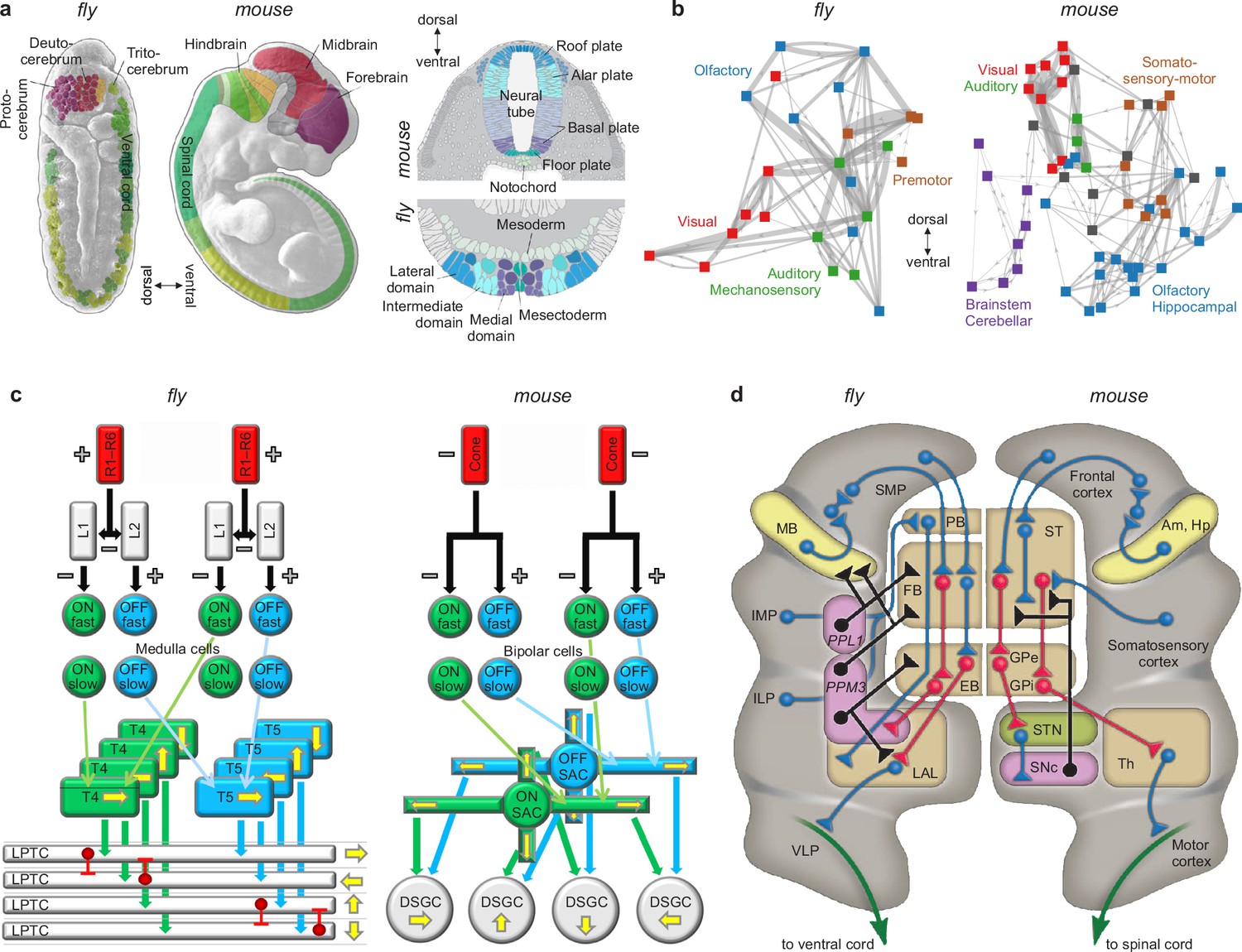
Similarities of development and structure in mice and flies.
(a) Conserved rostrocaudal (nose-to-tail, left panels) and dorsoventral (back-to-belly, right panels) patterns of neural gene expression in developing flies and mice. Matching colors denote homologous genes. Gene names not shown. (b) Conserved gross organization of regional modules in adult flies and mice. Note that, relative to flies, the organization of (a) expressed neural genes and (b) visual, auditory, and olfactory modules in mice is inverted dorsoventrally. This is a known developmental quirk (Held, 2017). (c) Similarities in the motion-detection circuits of flies and mice. R1–R6 photoreceptors in flies, and cone photoreceptors in mice, convert light into neural activity. Each photoreceptor has a distinct receptive field that responds to spatially distinct light stimuli. Parallel ON and OFF pathways in both animals extract motion signals from this activity. These pathways start with L1/L2 lamina monopolar cells in flies, and directly with photoreceptors in mice. Cells in the ON pathway depolarize, and cells in the OFF pathway repolarize, in response to increased visual input. Moreover, distinct cells within each pathway may respond to input on fast or slow timescales. T4/T5 interneurons in flies, and starburst amacrine interneurons (SACs) in mice, detect motion in each pathway by integrating fast and slow responses associated with specific receptive fields. Finally, lobular plate tangential cells (LPTCs) in flies, and ON-OFF direction-selective ganglion cells (DSGCs) in mice, recombine motion signals from the ON and OFF pathways. +/− denote excitation/inhibition, and yellow arrows denote four directions of motion. (d) Proposed homologies between the action-selection circuits of flies and mice. The alignment emphasizes the shared function of individual areas and of excitatory or modulatory (blue), inhibitory (red), dopaminergic (black), and descending (green) projections. In flies, action selection centers on the central complex. The central complex includes the protocerebral bridge (PB), the fan-shaped body (FB), and the ellipsoid body (EB). In mice, action selection centers on the basal ganglia. The basal ganglia include the striatum (ST) and the external and internal globus pallidi (GPe and GPi). The central complex receives direct projections from sensory areas, the intermediate and inferior lateral protocerebra (IMP and ILP). It also receives direct projections from an association area, the superior medial protocerebrum (SMP). Finally, it receives indirect projections, via the SMP, from a learning area, the mushroom body (MB). Correspondingly, the basal ganglia receive direct projections from sensory and association areas in the cortex and indirect projections, via association cortex, from learning areas (the amygdala and hippocampus, Am and Hp). The central complex projects to the ventral cord via the lateral accessory lobes (LAL) and the motor ventrolateral protocerebra (VLP). Similarly, the basal ganglia project to the spinal cord via the thalamus and the motor cortex. Finally, in both cases, dopamine plays an important modulatory role. It acts via PPL1 and PPM3 neurons in flies, and via the substantia nigra pars compacta (SNc) in mice. Note also that the gall (not shown) may be a fly homolog of the mouse suprathalamic nucleus (STN, Fiore et al., 2015). Panel (a) is reproduced from Figure 1 of Bailly et al., 2013. Panel (b) is adapted from Figure 1b of Rubinov, 2016. Panel (c) is reproduced from Figure 5 of Borst and Helmstaedter, 2015. Panel (d) is adapted from Figure 2 of Strausfeld and Hirth, 2013.
© 2015, Springer Nature. Panel (c) is reproduced from Figure 5 of Borst and Helmstaedter, 2015, with permission from Springer Nature. It is not covered by the CC-BY 4.0 license and further reproduction of this panel would need permission from the copyright holder.
© 2013, Science. Panel (d) is reproduced from Figure 2 of Strausfeld and Hirth, 2013. It is not covered by the CC-BY 4.0 license and further reproduction of this panel would need permission from the copyright holder.
Appendix 1—figure 1
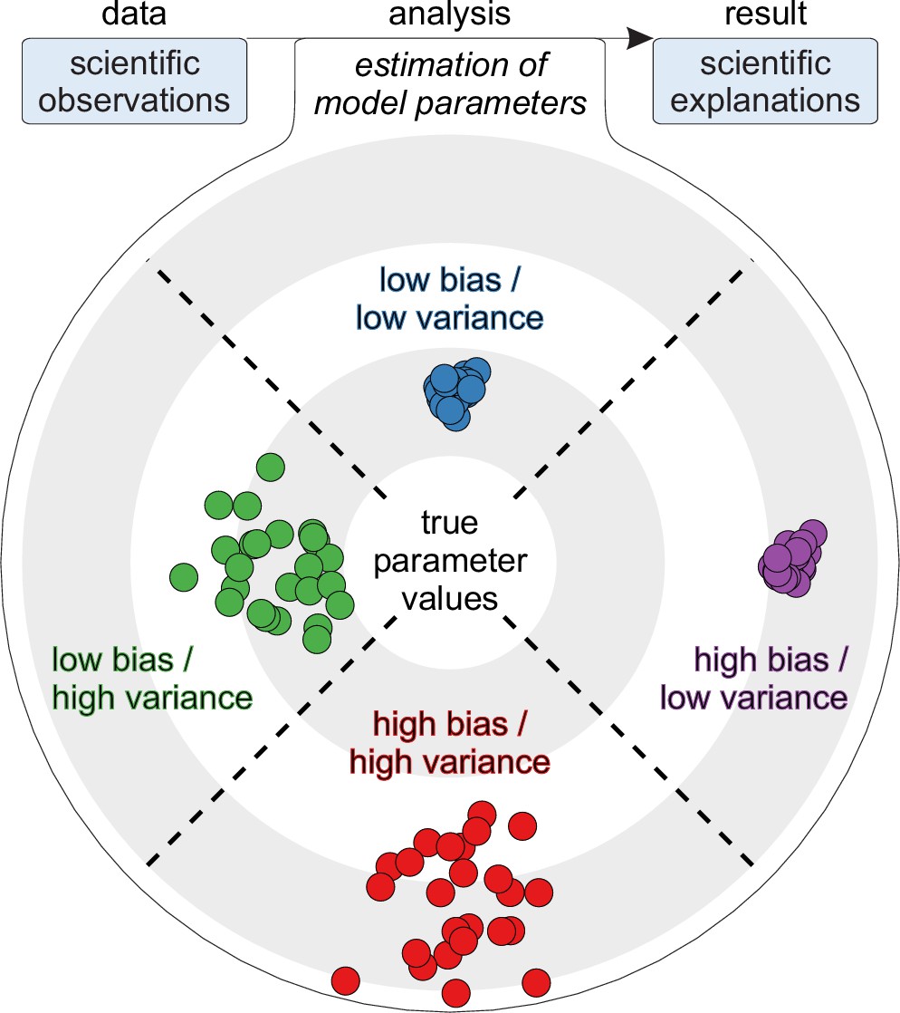
Statistical perspective on trueness and precision.
Top (flowchart): Analyses as parameter estimates of explanatory models. Bottom (target): Four example parameter estimates with distinct precision and trueness profiles (colored dots). True parameter values denote true explanations and not true predictions. High-bias estimates denote explanations that have low relative trueness. By contrast, high-variance estimates denote explanations that have low precision.
Appendix 5—figure 1
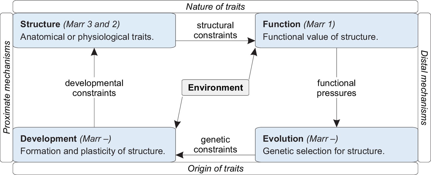
A framework for integrating existing knowledge.
Tinbergen’s four levels of analysis (blue boxes) organized along dimensions that reflect Mayr’s distinction between proximal and distal mechanisms. Arrows denote interactions (pressures or constraints) between individual levels. Laland et al., 2011, Bateson and Laland, 2013, Krakauer et al., 2017, and Mobbs et al., 2018 provide additional discussions of this framework.
Tables
Table 1
Definitions of terms.
| Term | Definition |
|---|---|
| Principle of parsimony (Occam’s razor) | An assertion that all else being equal, models with fewer redundant features are likely to be truer than rival models (Baker, 2022). This assertion reflects an objective preference for parsimony rather than a subjective preference for simplicity or elegance. In this way, and contrary to misconception, the principle of parsimony does not imply that reality, or its truest models, are simple or elegant. |
| Trueness (bias) | Distance between expected and true estimates of model parameters (ISO, 1994). True values of model parameters are typically inaccessible, and trueness (bias) can therefore be defined only in relative terms. The principle of parsimony asserts that all else being equal, models with fewer redundant features have truer (less biased) parameter estimates relative to rival models. |
| Precision (variance) | Expected distance between repeated estimates of model parameters (ISO, 1994). Precision (variance) does not require knowledge of the true values of model parameters and can therefore be defined in absolute terms. The problem of irreplicable results (Ioannidis, 2005) is primarily a problem of precision (variance). |
| Circular analysis | An analysis that first tests a model in a way that almost invariably accepts the model and then accepts the model on the basis of this test. This definition includes circular analyses of knowledge that accept overspecified models or redundant (less true) explanations. It also includes circular analyses of noise that accept overfitted models or irreplicable (less precise) explanations (Kriegeskorte et al., 2009). |
| Neural circuits or brain networks | Groups of connected neurons or brain regions that mediate function. This definition does not intend to make analogies between groups of neurons or brain regions, and electronic circuits or artificial neural networks (Rubinov, 2015). |
| Function | Behavior and other action that helps animals to survive and reproduce (Roux, 2014). This definition excludes physiological phenomena that lack such useful action. |
| Structure | Anatomical or physiological organization. This definition encompasses all physiological phenomena, including phenomena that lack known function. |
| Development | Formation of structure before and after birth. This definition includes plasticity and therefore encompasses learning and memory. |
Table 2
Example deepities.
| Deepity | Direct meaning | Implicit allusion |
|---|---|---|
| Neural computation (Churchland and Sejnowski, 2016) | Transformation of sensory input to behavioral output. | Computer-like transformation of sensory input to behavioral output. |
| Neural representation, code, or information (Baker et al., 2022; Brette, 2019; Nizami, 2019) | Patterns of neuronal activity that correlate with, or change in response to, sensory input. | Internal representations or encodings of information about the external world. |
| Neural networks (Bowers et al., 2022) | Artificial neural networks (machine-learning models). | Biological neural networks. |
| Necessity and sufficiency (Yoshihara and Yoshihara, 2018) | The induction or suppression of behavior through stimulation or inhibition of neural substrate. | Logical equivalence between behavior and neural substrate. |
| Functional connectivity (Reid et al., 2019) | Correlated neural activity. | Neural connectivity that causes function. |
| Complexity (Merker et al., 2022) | Patterns of neural structure that are neither ordered nor disordered. | Patterns of neural structure that are fundamentally important. |
| Motifs | Repeating patterns of brain-network connectivity. | Motifs of neural computation. |
| Efficiency | Communication between pairs of brain nodes via algorithmic sequences of connections. | Efficiency of neural communication. |
| Modularity | Propensity of brain networks to be divided into clusters. | Propensity of brain networks to be robust or evolvable. |
| Flexibility | Propensity for brain nodes to dynamically switch their cluster affiliations. | Propensity for cognitive flexibility. |
| The brain is a network, like many other natural and synthetic systems. | The brain consists of connected elements, like many other natural and synthetic systems. | The brain shares functional network principles with many natural and synthetic systems. |
| Brain disorders are disconnection syndromes. | Brain disorders are correlated with brain-network abnormalities. | Brain disorders are caused by brain-network abnormalities. |
Table 3
Example stories.
| Concept | Initial narrative of optimality | Evidence of suboptimality (strong but unviable null model) | Restoration of optimality through the inclusion of an ad hoc tradeoff | Alternative benchmark narrative (strong and viable null model) |
|---|---|---|---|---|
| Criticality (Fontenele et al., 2019; Wilting and Priesemann, 2019; Nanda et al., 2023) | Brain activity always and exactly balances between order and disorder. This allows it to optimize information transmission and storage. | Brain activity does not always or exactly balance between order and disorder. | Brain activity optimizes the tradeoffs between the benefits of criticality and the competing benefits of flexibility or stability. | Brain activity avoids the extremes of overinhibition and overexcitation and is not optimal over and above this avoidance-of-extremes baseline. |
| Predictive coding (Sun and Firestone, 2020; Van de Cruys et al., 2020; Seth et al., 2020; Cao, 2020) | Brain activity aims to optimally predict incoming sensory input. | Brain activity optimally predicts sensory input in dark and quiet spaces. Despite this, animals tend not to seek out such spaces. | Brain activity aims to optimize the tradeoffs between predictions that are accurate and predictions that are motivational. | Brain activity reacts to sensory input but does not aim to optimally predict this input. |
| Wiring minimization (Markov et al., 2013; Bullmore and Sporns, 2012; Rubinov, 2016) | Brain-network structure globally minimizes wiring cost and therefore optimizes wiring economy. | Brain-network structure does not globally minimize wiring cost. | Brain-network structure optimizes the tradeoffs between wiring cost and communication efficiency. | Brain networks have long connections that enable specific sensory-motor function but do not optimize global communication. |
Table 4
Example features and statistics.
| Model feature | Example statistic |
|---|---|
| Sensory-motor interactions | Connectivity and activity statistics of functional circuits. |
| Excitation/inhibition balance | 1/f power-spectral slopes (Gao et al., 2017). |
| Node connectivity | Degree-distribution statistics (Clauset et al., 2009). |
| Network clusters | Within-module densities (Fortunato, 2010). |
| Tuning representations | Tuning-curve statistics (Kriegeskorte and Wei, 2021). |
| Manifold representations | Persistent-homology barcodes (Ghrist, 2008). |
| Oscillations | Frequency-specific amplitudes and phases (Donoghue et al., 2020). |
| Criticality | Avalanche exponents (Sethna et al., 2001). |
| Small worlds | Small-world statistics (Bassett and Bullmore, 2017). |
| Cores/clubs | Within-core densities (Csermely et al., 2013). |
| Network controllability | Network-controllability statistics (Pasqualetti et al., 2014). |
Table 5
Examples of impactful advances.
| Advance | Nature of impact |
|---|---|
| Discoveries | Revisions of benchmark models (typically rare). |
| Null results | Rejections of previously promising speculative models. |
| Exploratory advances | Formulations of newly promising speculative models. |
| Conceptual advances | Discoveries of explanatory gaps that enable exploratory advances. |
| Methodological advances | Improvements in data or analysis that support all the other advances. |
Appendix 2—table 1
Weak-severity requirement and circular analysis.
| Weak-severity requirement (Mayo) | Circular analysis (this work) |
|---|---|
Bad evidence, no test.
| General definition (weak evidence of progress).
|
| N/A. The framework of severe testing, and the weak-severity requirement, do not specifically consider the problem of redundant explanations. | Specific definition (strong evidence of stagnation).
|
Appendix 2—table 2
Strong severity and unified analysis.
| Strong-severity requirement (Mayo) | Unified analysis (this work) |
|---|---|
Evidence from survival of stringent scrutiny.
| Evidence of genuinely new discovery.
|
Appendix 3—table 1
Two types of circular analysis.
| Circular analysis of noise | Circular analysis of knowledge | |
|---|---|---|
| Conceptual problem | Explanation of the same aspect of the data twice: first as noise, and second as a new discovery non-independent of this noise. | Explanation of the same aspect of the data twice: first as existing knowledge, and second as new discovery redundant with this knowledge. |
| Statistical problem | Model overfitting that results in high variance (low precision) of estimated model parameters. | Model overspecification that results in high bias (low trueness) of estimated model parameters. |
| Statistical solution | Tests of independence against sampled data in which all benchmark (noise) features are maximally random and all other aspects of the data are preserved. | Tests of non-redundancy against sampled data in which all benchmark (existing knowledge) features are preserved and all other aspects of the data are maximally random. |
Additional files
Download links
A two-part list of links to download the article, or parts of the article, in various formats.
Downloads (link to download the article as PDF)
Open citations (links to open the citations from this article in various online reference manager services)
Cite this article (links to download the citations from this article in formats compatible with various reference manager tools)
Circular and unified analysis in network neuroscience
eLife 12:e79559.
https://doi.org/10.7554/eLife.79559


