Arnold tongue entrainment reveals dynamical principles of the embryonic segmentation clock
- European Molecular Biology Laboratory (EMBL), Developmental Biology Unit, Germany
- McGill University, Canada
- European Molecular Biology Laboratory (EMBL), Transgenic Service, Germany
Figures
Figure 1 with 1 supplement
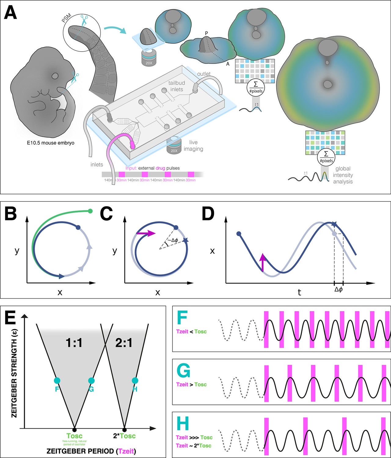
Entrainment of an embryonic oscillator with a zeitgeber: setup and theory.
(A) Schematic of the experimental entrainment setup using a microfluidics device previously described in Sonnen et al., 2018, and an overview of the analysis approach used in this present study. (1) The posterior presomitic mesoderm (PSM) is recovered from E10.5 mouse embryo and used in a quasi-two-dimensional segmentation assay (‘2D-assay’) (Lauschke et al., 2013). (2) The embryonic tissue is loaded into a microfluidics device bonded to fibronectin-coated cover glass, and is imaged using a ×20 objective at 37°C and 5% CO2. (3) Simultaneously, the 2D-assay is subjected to periodic pulses of a drug (e.g. DAPT for Notch signaling), which serves as zeitgeber. (4) Using dynamic fluorescent reporter for segmentation clock genes (e.g. LuVeLu for Notch signaling), we quantify endogenous signaling oscillations during the experiment. (5) We generate a single timeseries using reporter signal from the entire sample (‘global region of interest [ROI]’) that allows to quantify the segmentation clock rate and rhythm (see validation in Figure 2 and Figure 7—figure supplement 3). Illustration by Stefano Vianello. A photo of the actual microfluidics device and its design are shown in Figure 1—figure supplement 1. (B) Abstract definition of phase: two different points in the plane have the same phase if they converge on the same point on the limit cycle (indicated in gray). (C) Perturbations change the phase of the cycle by an increment (here phase is defined by the angle in the plane). (D) Time courses with similar perturbation as C showing the oscillations of and phase difference . (E) Illustration of generic Arnold tongues, plotted as a function of zeitgeber strength () and zeitgeber period (), mapping entrainment where the entrained oscillator (with natural period of ) goes through cycle/s for every cycle/s of the zeitgeber. Three different points in the 1:1 and 2:1 Arnold tongues are specified with corresponding graphical illustration of an autonomous oscillator as it is subjected to zeitgeber with different periods (): when is less than (F), when is greater than (G), and when is much much greater than but is close to twice of (H). Free-running rhythm of the oscillator (i.e. before perturbation) is marked by a dashed line, while solid line illustrates its rhythm during perturbation with zeitgeber. Magenta bars represent the zeitgeber pulses. Illustration by Stefano Vianello.
Figure 1—figure supplement 1
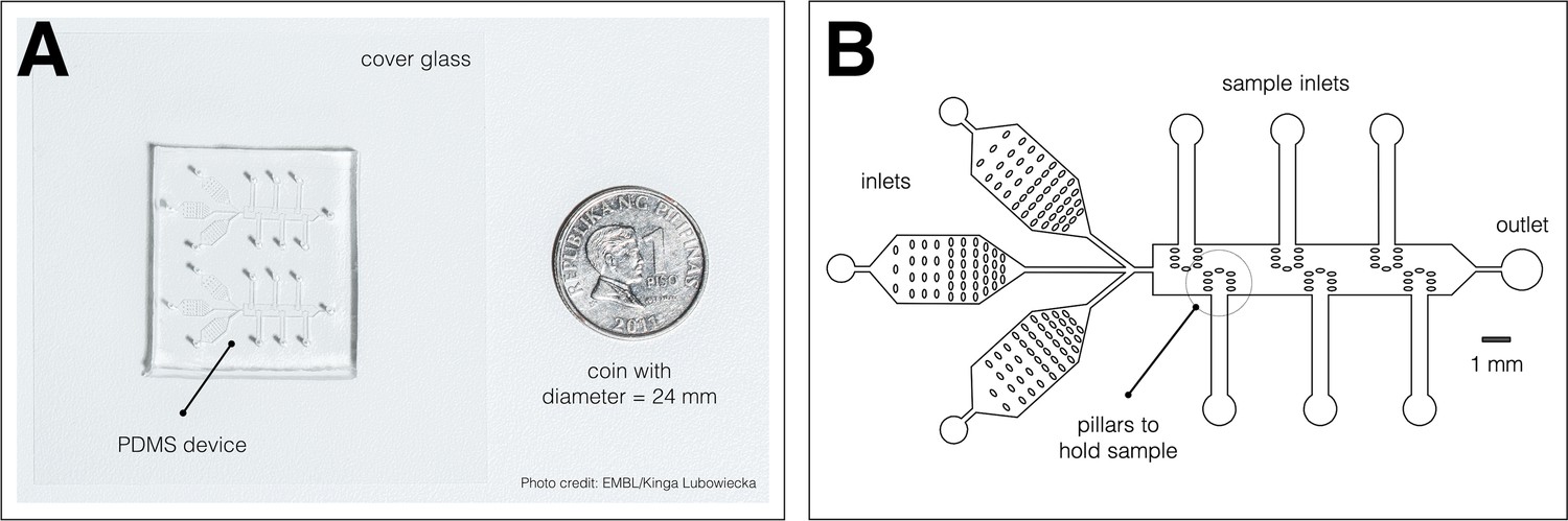
Microfluidics device.
A microfluidics device for simultaneous culture, imaging, and entrainment of the segmentation clock in 2D-assays. (A) Photo of the chip, previously described in Sonnen et al., 2018, bonded to cover glass and a coin (diameter: 24 mm) for scale. The split layout separating the upper and lower channel systems allows simultaneous delivery of drug and DMSO control to samples on opposite sides of the same device. Photo credit: EMBL/Kinga Lubowiecka. (B) Design of the microfluidics chip, showing inlets for medium and drug, inlets for the samples, pillars to hold each sample, and an outlet.
Figure 2 with 4 supplements
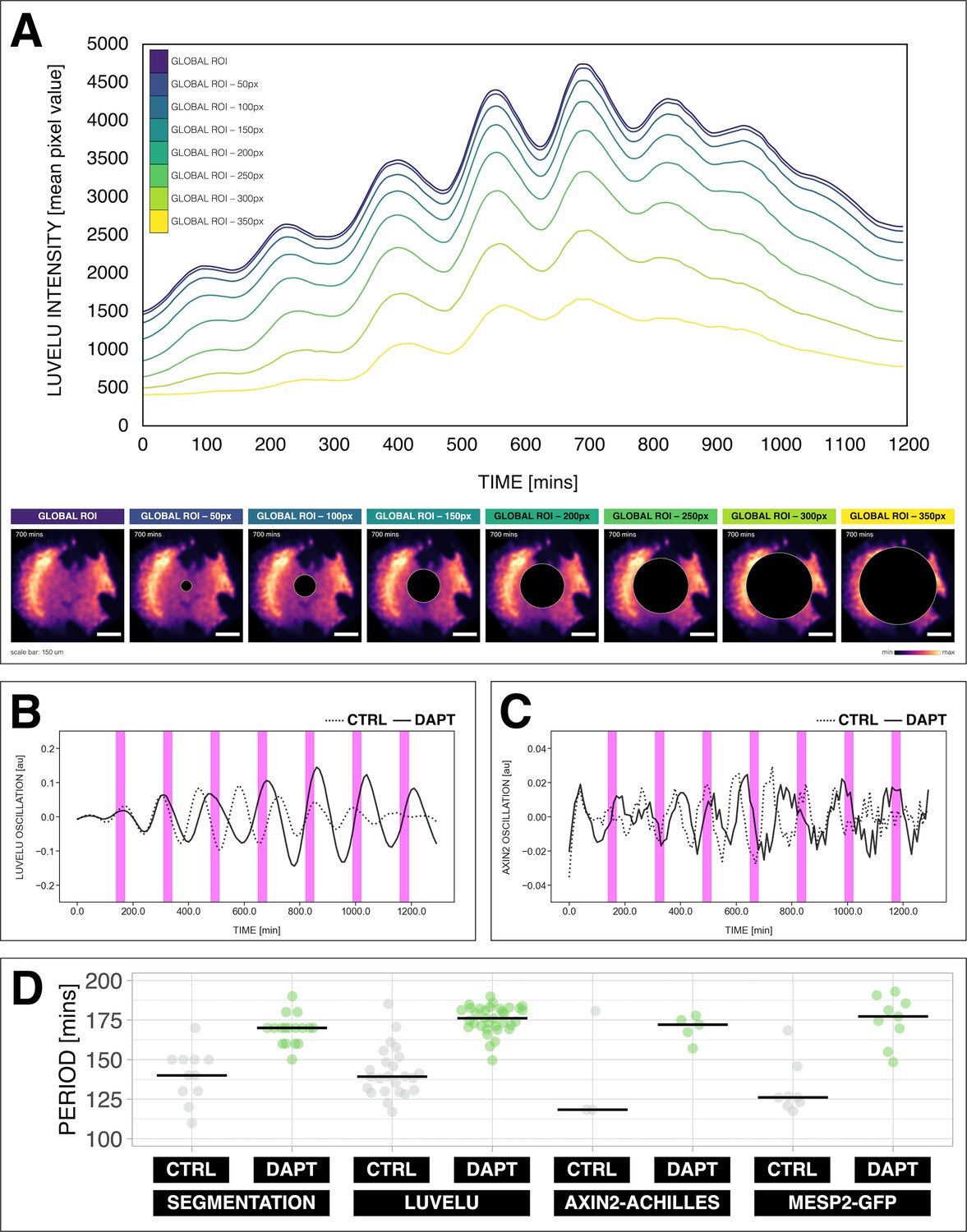
Quantifying the segmentation clock rhythm.
(A) Comparison of measurements obtained from a region of interest (ROI) spanning the entire field (‘global ROI’) with those obtained from ROIs in which central regions of increasing size were excluded. The excluded area is represented in terms of the diameter (in pixels, px) of a circular region at the center. The corresponding timeseries are shown in the top panel and marked with different colors. Bottom panel shows the global ROI and excluded region in a snapshot of signal of LuVeLu, a dynamic reporter of Notch signaling driven from the Lfng promoter (Aulehla et al., 2008), in a 2D-assay at 700 min from the start of the experiment. Henceforth, timeseries is obtained using ‘global ROI’, unless otherwise specified. (B) Detrended timeseries of the segmentation clock (obtained using global ROI) in 2D-assays, which express the LuVeLu reporter, subjected to 170 min periodic pulses (magenta bars) of either 2 µM DAPT (in solid line) or DMSO (for control, in dashed line). Timelapse movie and corresponding timeseries from global ROI are available at https://youtu.be/fRHsHYU_H2Q. (C) Detrended timeseries of Axin2-linker-Achilles reporter in 2D-assays, subjected to 170 min periodic pulses (magenta bars) of either 2 µM DAPT (in solid line) or DMSO (for control, in dashed line). (D) Period of morphological segment boundary formation, LuVeLu oscillation, Axin2-linker-Achilles oscillation, and rhythm of Mesp2-GFP in 2D-assays subjected to 170 min periodic pulses of either 2 µM DAPT (or DMSO for control). Each sample is represented as a dot, the median is denoted as a solid horizontal line. For morphological segment boundary formation, period was determined by taking the time difference between two consecutive segmentation events (for CTRL: 17 segmentation events in six samples from four independent experiments, and for DAPT: 24 segmentation events in seven samples from five independent experiments, with p-value < 0.001) in the brightfield channel. For period quantifications based the reporters, the mean period per sample from 650 to 850 min after start of the experiment was plotted. LuVeLu: (CTRL: n=24 and N=7) and (DAPT: n=34 and N=8) with p-value < 0.001, Axin2-linker-Achilles: (CTRL: n=3 and N=1) and (DAPT: n=5 and N=1) with p-value = 0.107, Mesp2-GFP: (CTRL: n=8 and N=3) and (DAPT: n=9 and N=3) with p-value = 0.01. Data were visualized using PlotsOfData (Postma and Goedhart, 2019). To calculate the p-value, two-tailed test for absolute difference between medians was done via a randomization method using PlotsOfDifferences (Goedhart, 2019). The timeseries and corresponding period evolution during entrainment, obtained from wavelet analysis, are in Figure 2—figure supplement 1A and Figure 2—figure supplement 1B, respectively. Timelapse movies are available at https://youtu.be/edFczx_-9hM and https://youtu.be/tQeBk0_U_Qo, respectively.
Figure 2—figure supplement 1
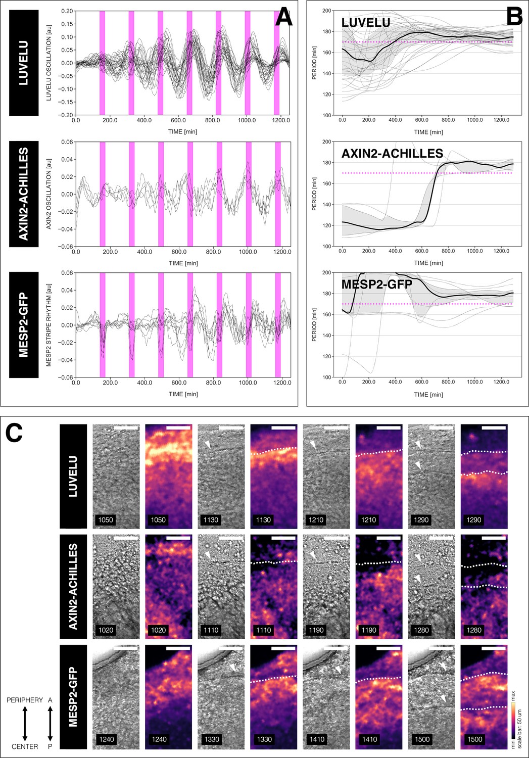
Different readouts of the segmentation clock.
The rhythms of different dynamic readouts of the entrained segmentation clock match. (A) Detrended timeseries of the segmentation clock in 2D-assays subjected to 170 min periodic pulses of 2 µM DAPT, and expressing either LuVeLu (Aulehla et al., 2008), Axin2-linker-Achilles, or Mesp2-GFP (Morimoto et al., 2006). Periodic pulses are indicated as magenta bars and the timeseries of each sample (for LuVeLu: n=34 and N=8, for Axin2-linker-Achilles: n=5 and N=1, for Mesp2-GFP: n=9 and N=3) is marked with a dashed line. The detrended timeseries for samples expressing LuVeLu is the same as the detrended timeseries for the DAPT condition in Figure 3A. (B) Period evolution during entrainment, obtained from wavelet analysis. The period evolution for each sample and the median of the periods are represented here as a dashed line and a solid line, respectively. The gray shaded area corresponds to the interquartile range. Magenta dashed line marks . The period evolution plot for samples expressing LuVeLu is the same as the period evolution plot for the DAPT condition in Figure 3B. (C) Snapshots of segmenting regions in 2D-assays subjected to 170 min periodic pulses of 2 µM DAPT, and expressing either LuVeLu (Aulehla et al., 2008), Axin2-linker-Achilles, or Mesp2-GFP (Morimoto et al., 2006), at different time points. Segment boundaries are marked with either white arrowheads (brightfield channel) or white dashed lines (reporter channel). Samples are re-oriented so that the top is toward the periphery and the bottom is toward the center of the 2D-assay. Time is indicated as minutes elapsed from the start of the experiment. Scale bar: 50 µm. Timelapse movies of 2D-assays expressing either Axin2-linker-Achilles or Mesp2-GFP subjected to said perturbation are available at https://youtu.be/edFczx_-9hM and https://youtu.be/tQeBk0_U_Qo, respectively.
Figure 2—video 1
E10.5 2D-assay, expressing LuVeLu, subjected to 170 min periodic pulses of 2 µM DAPT (or DMSO for control), with corresponding timeseries obtained using a global region of interest (ROI) spanning the entire field of view, available at https://youtu.be/fRHsHYU_H2Q.
Figure 2—video 2
E10.5 2D-assay, expressing Axin2-linker-Achilles, subjected to 170 min periodic pulses of 2 µM DAPT (or DMSO for control) available at https://youtu.be/edFczx_-9hM.
Figure 2—video 3
E10.5 2D-assay, expressing Mesp2-GFP, subjected to 170 min periodic pulses of 2 µM DAPT (or DMSO for control) available at https://youtu.be/tQeBk0_U_Qo.
Figure 3 with 2 supplements
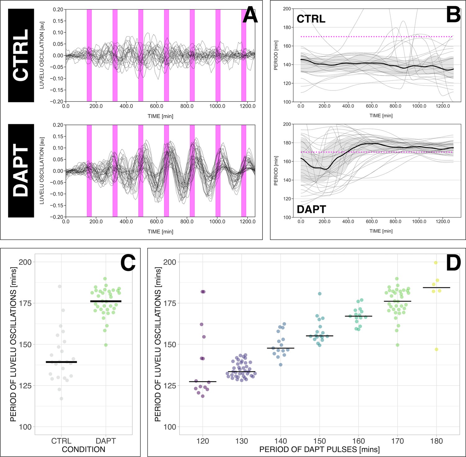
The segmentation clock can be locked to a wide range of entrainment periods.
(A) Detrended (via sinc filter detrending) timeseries of the segmentation clock in 2D-assays subjected to 170 min periodic pulses of 2 µM DAPT (or DMSO for controls). Periodic pulses are indicated as magenta bars and the timeseries of each sample (for CTRL: n=24 and N=7, for DAPT: n=34 and N=8) is marked with a dashed line. (B) Period evolution during entrainment, obtained from wavelet analysis. The period evolution for each sample and the median of the periods are represented here as a dashed line and a solid line, respectively. The gray shaded area corresponds to the interquartile range. Magenta dashed line marks . (C) Mean period from 650 to 850 min after start of the experiment of samples subjected to 170 min periodic pulses of 2 µM DAPT (or DMSO for controls), with p-value <0.001. Each sample is represented as a dot, while the median of all samples is denoted as a solid horizontal line. This plot is the same as the plot for the LuVeLu condition in Figure 2D. (D) Mean period from 650 to 850 min after start of the experiment of samples entrained to periodic pulses of 2 µM DAPT. Each sample is represented as a dot, while the median of all samples is denoted as a solid horizontal line. The period of the DAPT pulses is specified (for 120 min: n=14 and N=3, for 130 min: n=39 and N=10, for 140 min: n=15 and N=3, for 150 min: n=17 and N=4, for 160 min: n=15 and N=3, for 170 min: n=34 and N=8, for 180 min: n=6 and N=1). Data were visualized using PlotsOfData (Postma and Goedhart, 2019), and a summary is provided in Table 1. A similar plot including each condition’s respective control is in Figure 3—figure supplement 1. The analysis of period and wavelet power across time is summarized in Figure 3—figure supplement 2. To calculate the p-value, two-tailed test for absolute difference between medians was done via a randomization method using PlotsOfDifferences (Goedhart, 2019).
Figure 3—figure supplement 1
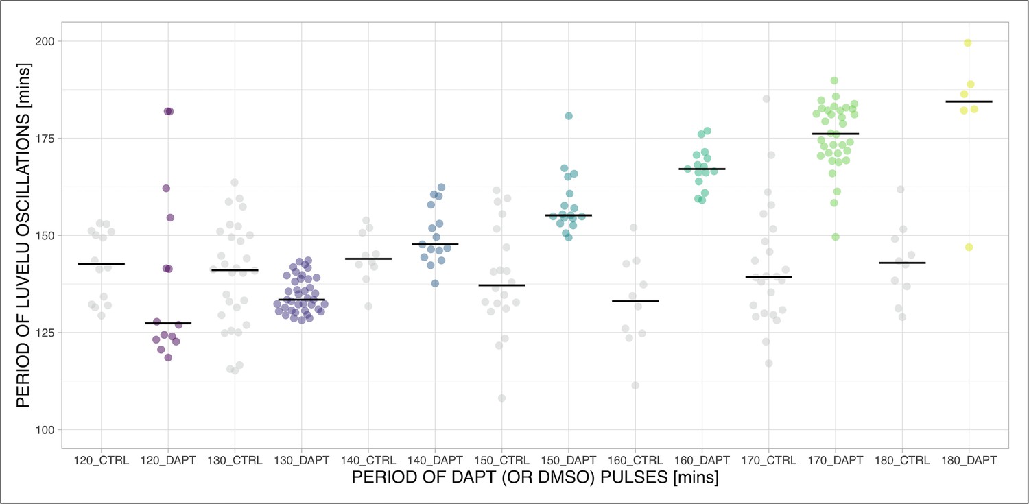
Speeding up and slowing down the period of the segmentation clock.
The period of the segmentation clock can both be sped up and slowed down by modulating the period of DAPT pulses. Mean period from 650 to 850 min after start of the experiment of samples subjected to periodic pulses of 2 µM DAPT (or DMSO for controls). Each sample is represented as a dot, while the median of all samples is denoted as a solid horizontal line. The period of the DAPT (or DMSO) pulses is specified. 120 min: (CTRL: n=14 and N=3) and (DAPT: n=14 and N=3) with p-value = 0.064, 130 min: (CTRL: n=30 and N=8) and (DAPT: n=39 and N=10) with p-value = 0.003, 140 min: (CTRL: n=10 and N=3) and (DAPT: n=15 and N=3) with p-value = 0.272, 150 min: (CTRL: n=20 and N=4) and (DAPT: n=17 and N=4) with p-value = 0.001, 160 min: (CTRL: n=10 and N=3) and (DAPT: n=15 and N=3) with p-value <0.001, 170 min: (CTRL: n=24 and N=7) and (DAPT: n=34 and N=8) with p-value <0.001, 180 min: (CTRL: n=10 and N=2) and (DAPT: n=6 and N=1) with p-value = 0.001. Data were visualized using PlotsOfData (Postma and Goedhart, 2019). To calculate p-values, two-tailed test for absolute difference between medians was done via a randomization method using PlotsOfDifferences (Goedhart, 2019).
Figure 3—figure supplement 2
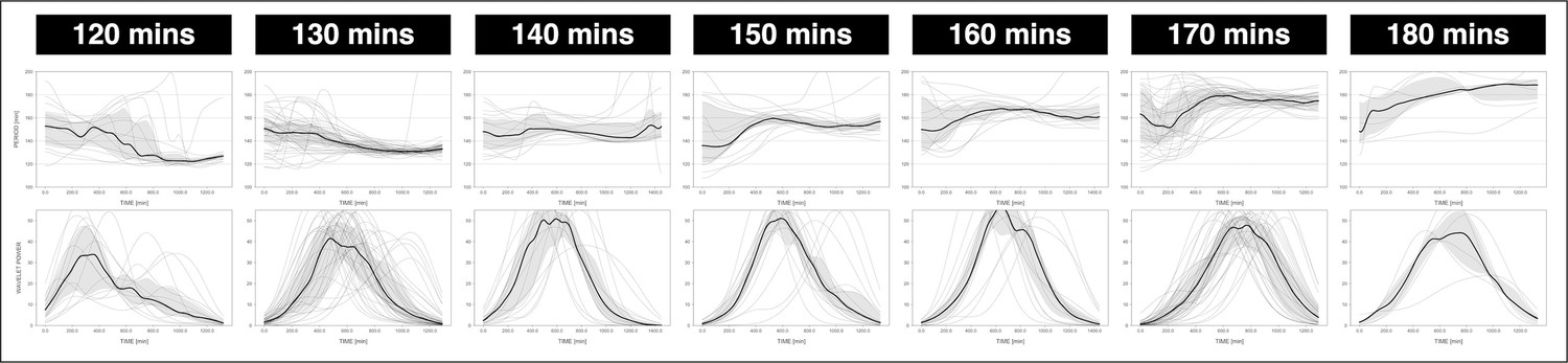
Locking of the segmentation clock to the period of the DAPT pulses.
The period of the segmentation clock becomes locked to the period of the DAPT pulses. The period and wavelet power of the oscillations, obtained via wavelet analysis, are plotted across time. Each sample and their median are represented here as a dashed line and a solid line, respectively. The gray shaded area corresponds to the interquartile range. The period of the 2 µM DAPT pulses is specified. 120 min: n=14 and N=3, 130 min: n=39 and N=10, 140 min: n=15 and N=3, 150 min: n=17 and N=4, 160 min: n=15 and N=3, 170 min: n=34 and N=8, 180 min: n=6 and N=1. The period evolution plots for the 130 and 170 min conditions are the same as the period evolution plots for the 2 µM condition in Figure 4—figure supplement 1A and Figure 4B, respectively.
Figure 4 with 2 supplements
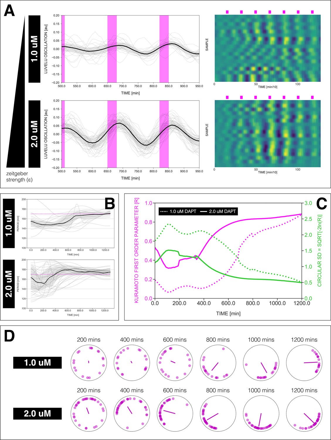
Effect of varying DAPT concentrations on entrainment dynamics.
(A) Left: Detrended (via sinc filter detrending) timeseries of the segmentation clock in 2D-assays entrained to 170 min periodic pulses of either 1 or 2 µM DAPT, zoomed in from 500 to 950 min. Periodic pulses are indicated as magenta bars and the timeseries of each sample (for 1 µM: n=18 and N=5, for 2 µM: n=34 and N=8) is marked with a dashed line. The median of the oscillations is represented here as a solid line, while the gray shaded area denotes the interquartile range. Right: Detrended (via sinc filter detrending) timeseries of the segmentation clock in 2D-assays entrained to 170 min periodic pulses of either 1 µM (n=18 and N=5) or 2 µM (n=18 and N=8) DAPT represented as heatmaps, generated using PlotTwist (Goedhart, 2020). Periodic pulses are indicated as magenta bars. Each row corresponds to a sample. (B) Period evolution during entrainment, obtained from wavelet analysis. The period evolution for each sample and the median of the periods are represented here as a dashed line and a solid line, respectively. The gray shaded area corresponds to the interquartile range. The plot for the 2 µM condition is the same as the plot for the DAPT condition in Figure 3B. Magenta dashed line marks . (C) Evolution of first Kuramoto order parameter () in magenta and circular standard deviation () in green over time, showing change in coherence of multiple samples during the experiment. An equal to 1.0 means that samples are in-phase. is equal to . (D) Polar plots at different timepoints showing phase of each sample and their first Kuramoto order parameter, represented as a magenta dot along the circumference of a circle and a magenta line segment at the circle’s center, respectively. A longer line segment corresponds to a higher first Kuramoto order parameter, and thus to more coherent samples. The direction of the line denotes the vectorial average of the sample phases. Time is indicated as minutes elapsed from the start of the experiment.
Figure 4—figure supplement 1
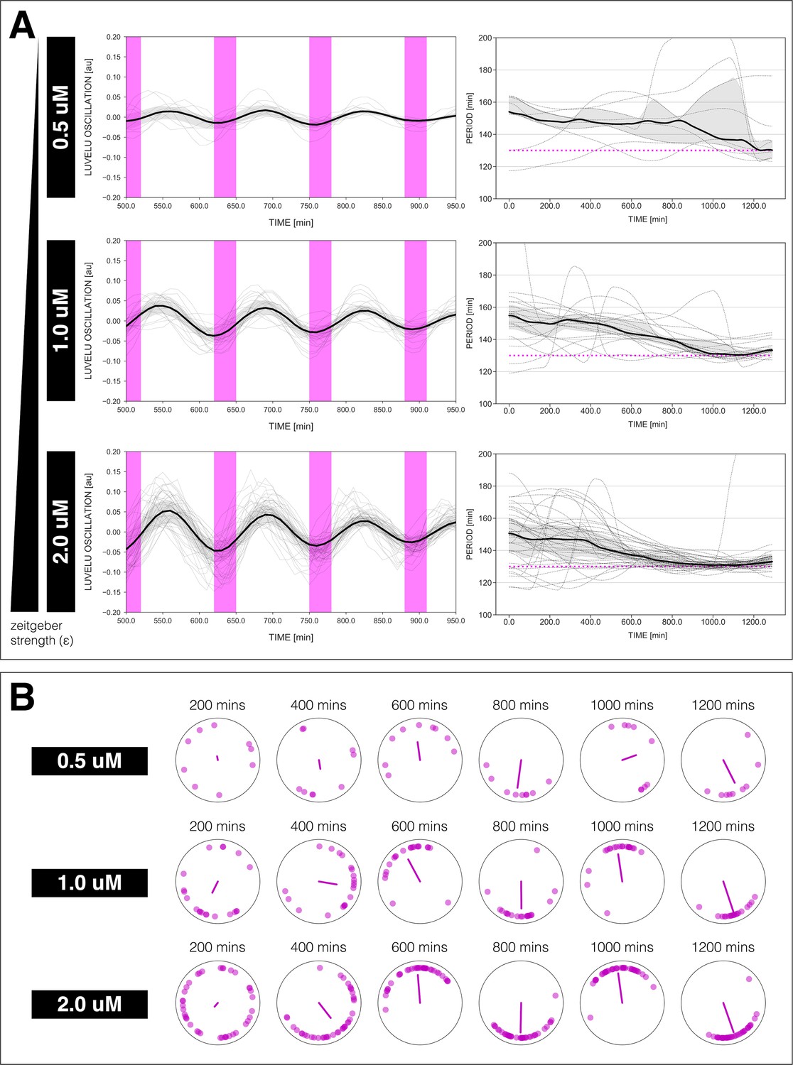
Changing the concentration of DAPT affects entrainment.
Changing the concentration of DAPT, equivalent to changing zeitgeber strength, affects entrainment of the segmentation clock to 130 min periodic DAPT pulses. (A) Left: Detrended (via sinc filter detrending) timeseries of the segmentation clock in 2D-assays entrained to 130 min periodic pulses of either 0.5, 1, or 2 µM DAPT, zoomed in from 500 to 950 min. Periodic pulses are indicated as magenta bars and the timeseries of each sample (for 0.5 µM: n=9 and N=2, for 1 µM: n=20 and N=4, for 2 µM: n=39 and N=10) is marked with a dashed line. The median of the oscillations is represented here as a solid line, while the gray shaded area denotes the interquartile range. Right: Period evolution during entrainment, obtained from wavelet analysis. The period evolution for each sample and the median of the periods are represented here as a dashed line and a solid line, respectively. The gray shaded area corresponds to the interquartile range. Magenta dashed line marks . (B) Polar plots at different timepoints showing phase of each sample and their first Kuramoto order parameter, represented as a magenta dot along the circumference of a circle and a magenta line segment at the circle’s center, respectively. A longer line segment corresponds to a higher first Kuramoto order parameter, and thus to more coherent samples. The direction of the line denotes the vectorial average of the sample phases. Time is indicated as minutes elapsed from the start of the experiment.
Figure 4—figure supplement 2
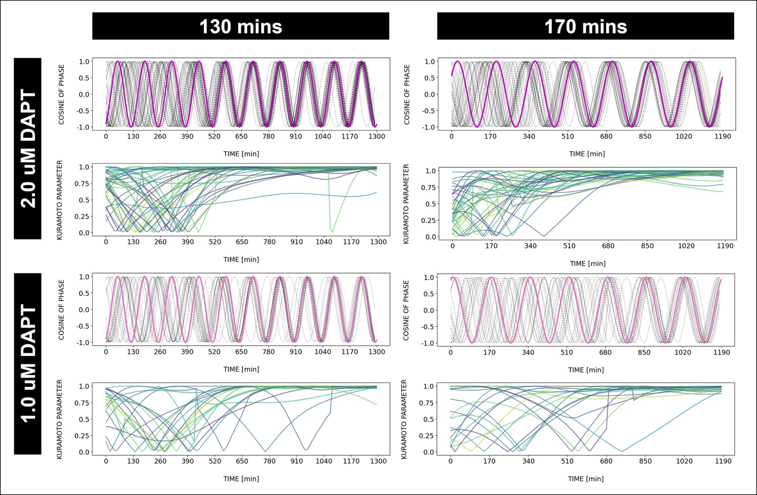
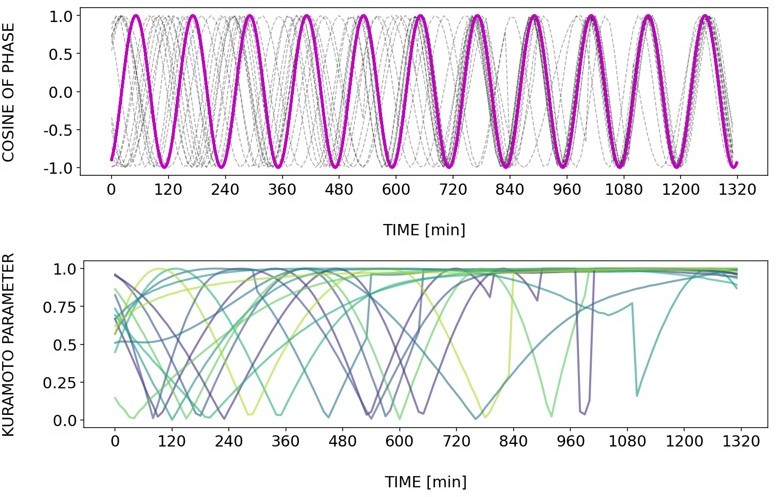
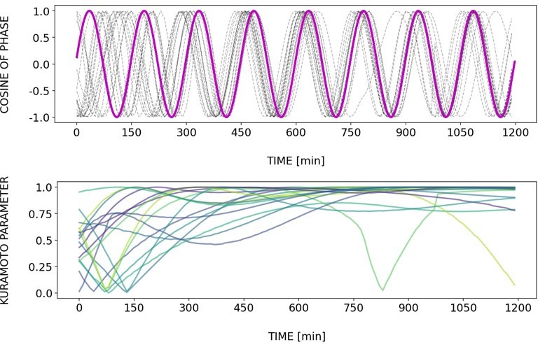
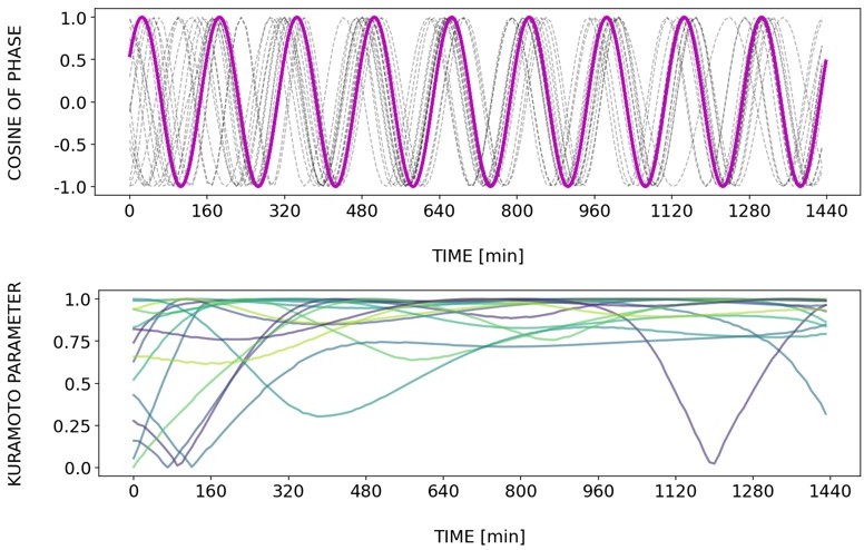
Dynamics and variability of entrainment.
Dynamics and variability of entrainment. We represent the zeitgeber signal as a continuous uniformly increasing phase (‘zeitgeber time’) with period . The initial condition for is chosen so that the zeitgeber phase at the moment of the last pulse is matching the experimental entrainment phase for each . We plot the corresponding for each sample (dotted lines) and the zeitgeber phase (solid lines). To quantify how well each sample is following the zeitgeber, we compute the Kuramoto parameter: , where is the phase of sample . Convergence to 1 of the Kuramoto parameter indicates the establishment of a stable phase relation between the sample and zeitgeber pulses, indicative of entrainment. As seen from the plots, at lower concentration of DAPT samples take a longer time on average to reach entrainment.
Figure 5
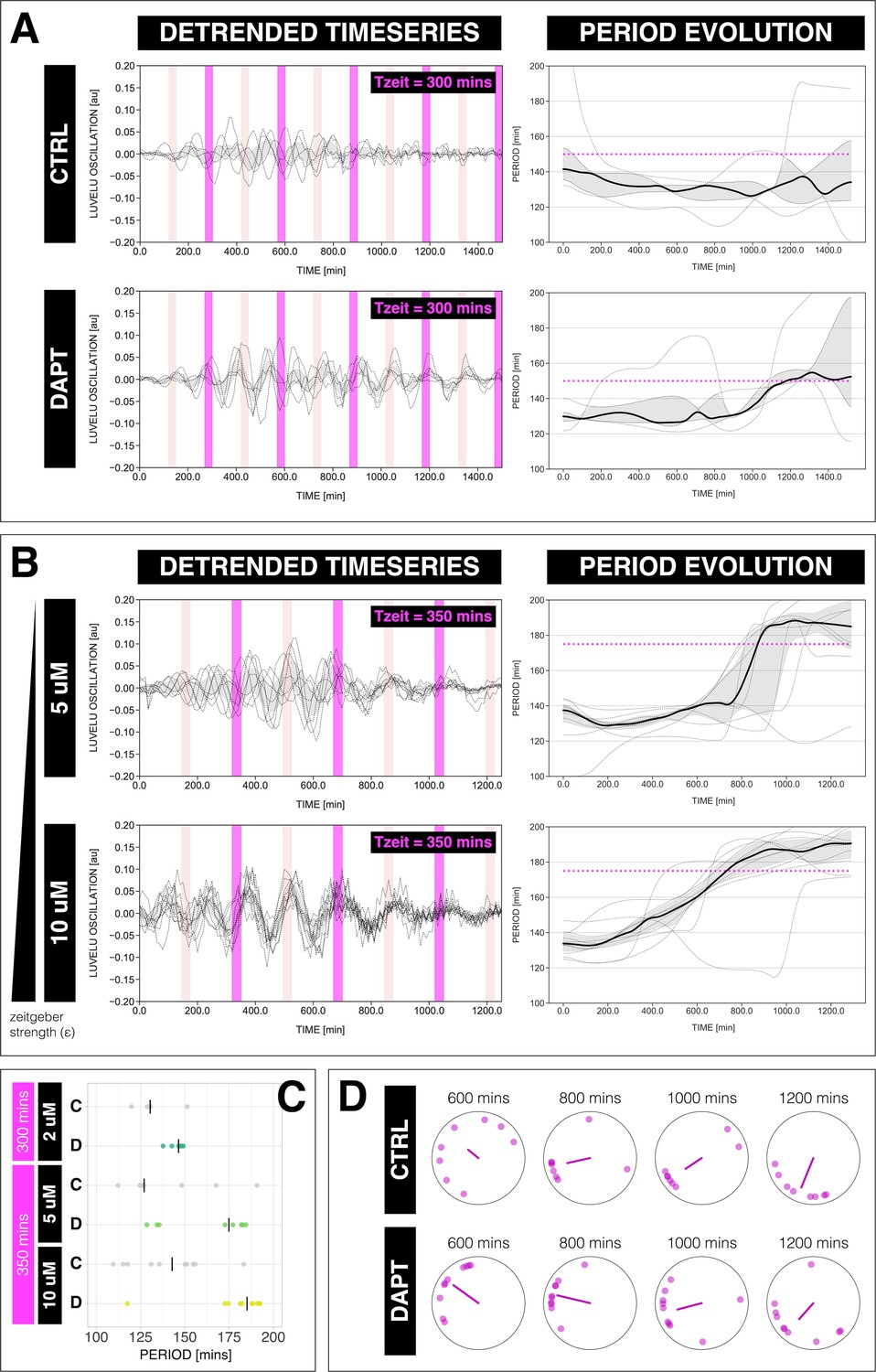
The segmentation clock can be entrained to a higher order.
(A) Left: Detrended (via sinc filter detrending) timeseries of the segmentation clock in 2D-assays subjected to 300 min periodic pulses of 2 µM DAPT (or DMSO for controls). Periodic pulses are indicated as magenta bars and the timeseries of each sample (for CTRL: n=5 and N=1, for DAPT: n=5 and N=1) is marked with a dashed line. The gray shaded area denotes the interquartile range. Hypothetical pulses at half the zeitgeber period are indicated as light pink bars. Right: Period evolution during entrainment, obtained from wavelet analysis. The period evolution for each sample and the median of the periods are represented here as a dashed line and a solid line, respectively. The gray shaded area corresponds to the interquartile range. Magenta dashed line marks . (B) Left: Detrended (via sinc filter detrending) timeseries of the segmentation clock in 2D-assays subjected to 350 min periodic pulses of either 5 µM DAPT or 10 µM DAPT. Periodic pulses are indicated as magenta bars and the timeseries of each sample (for 5 µM DAPT: n=8 and N=2, for 10 µM DAPT: n=10 and N=2) is marked with a dashed line. The gray shaded area denotes the interquartile range. Hypothetical pulses at half the zeitgeber period are indicated as light pink bars. Right: Period evolution during entrainment, obtained from wavelet analysis. The period evolution for each sample and the median of the periods are represented here as a dashed line and a solid line, respectively. The gray shaded area corresponds to the interquartile range. Magenta dashed line marks . (C) Mean period either from 1000 to 1150 min (for min) or from 800 to 950 min (for min) after start of the experiment of samples subjected to periodic pulses of DAPT (or DMSO for controls). Each sample is represented as a dot, while the median of all samples is denoted as a solid vertical line. For 300 min 2 µM DAPT: (CTRL: n=5 and N=1) and (DAPT: n=5 and N=1) with p-value = 0.191, for 350 min 5 µM DAPT: (CTRL: n=7 and N=2) and (DAPT: n=8 and N=2) with p-value = 0.049, for 350 min 10 µM DAPT: (CTRL: n=10 and N=2) and (DAPT: n=10 and N=2) with p-value = 0.016. The period and concentration of the DAPT pulses are specified. Data were visualized using PlotsOfData (Postma and Goedhart, 2019). To calculate p-values, two-tailed test for absolute difference between medians was done via a randomization method using PlotsOfDifferences (Goedhart, 2019). (D) Polar plots at different timepoints showing the phase of each sample in (A) and the first Kuramoto order parameter, represented as a magenta dot along the circumference of a circle and a magenta line segment at the circle’s center, respectively. A longer line segment corresponds to a higher first Kuramoto order parameter, and thus to more coherent samples. The direction of the line denotes the vectorial average of the sample phases. Time is indicated as minutes elapsed from the start of the experiment.
Figure 6
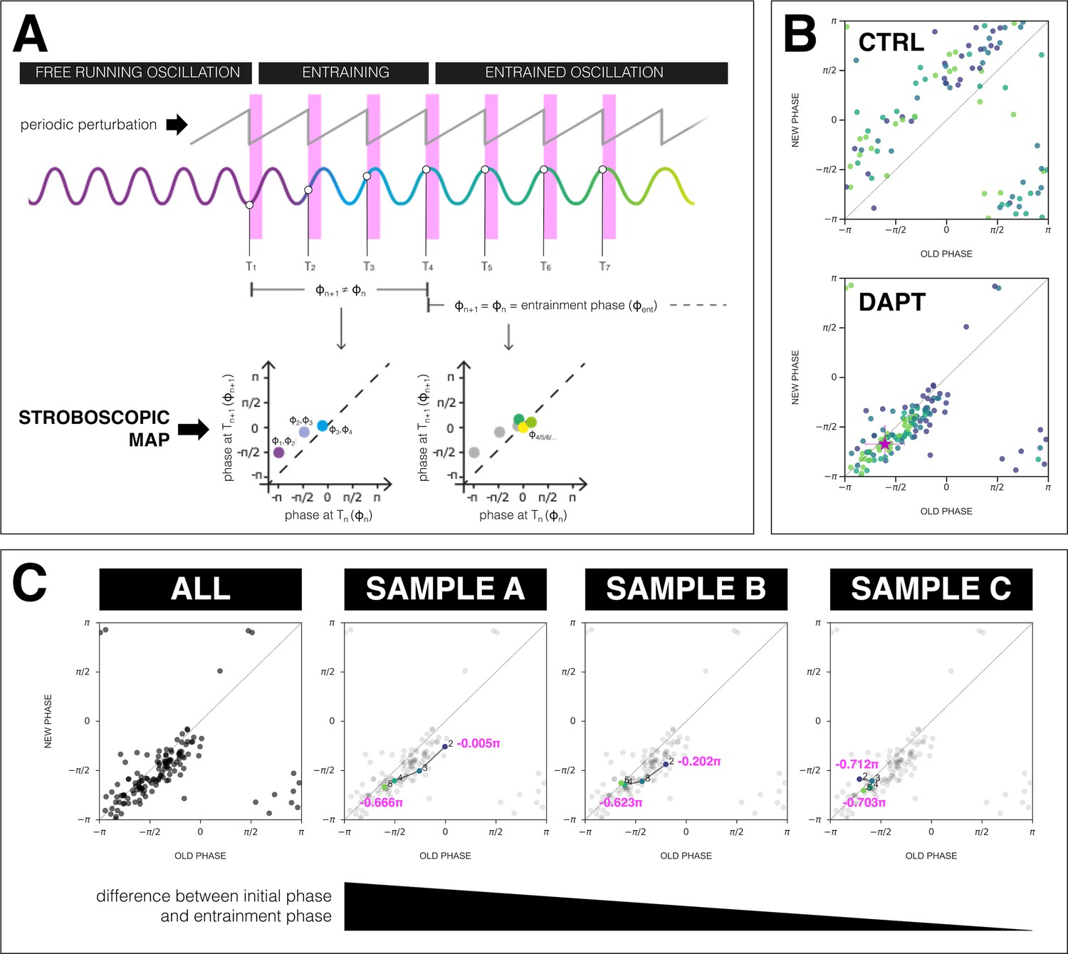
The segmentation clock establishes a stable phase relationship with the zeitgeber.
(A) Schematic of how to generate a stroboscopic map, where the phase of the segmentation clock just before a DAPT pulse (old phase, ) is iteratively plotted against its phase just before the next pulse (new phase, ).The position of each point in a stroboscopic map thus denotes a stepwise change in phase of the segmentation clock as it undergoes entrainment to the zeitgeber. Upon entrainment and phase-locking, the new phase is equal to the old phase, thus marking a point that lies on the diagonal of the stroboscopic map. This point on the diagonal is the entrainment phase (). Illustration by Stefano Vianello. (B) Stroboscopic map of samples subjected to 170 min periodic pulses of 2 µM DAPT (or DMSO for controls). Colors mark progression in time, from purple (early) to yellow (late). Note that while in control samples, points remain above the diagonal (reflecting that endogenous oscillations run faster than min as shown in Figure 3B–C), in entrained samples, the measurements converge toward a point on the diagonal (i.e. the entrainment phase, ), showing phase-locking. This localized region marks the entrainment phase (). This is highlighted with a magenta star, which corresponds to the centroid . The centroid was calculated from the vectorial average of the phases of the samples at the end of the experiment, where xc = vectorial average of old phase, yc = vectorial average of new phase. The spread of the points in the region is reported in terms of the circular standard deviation (, where is the first Kuramoto order parameter). (C) Stroboscopic maps of the segmentation clock entrained to 170 min periodic pulses of 2 µM DAPT (n=34 and N=8), for all samples (ALL) and for three individual samples (SAMPLE A, SAMPLE B, SAMPLE C). The numbers and colors (from purple to yellow) denote progression in time. The initial phase (old phase at point 2) and the entrainment phase (new phase at point 5) of each sample are specified.
Figure 7 with 3 supplements
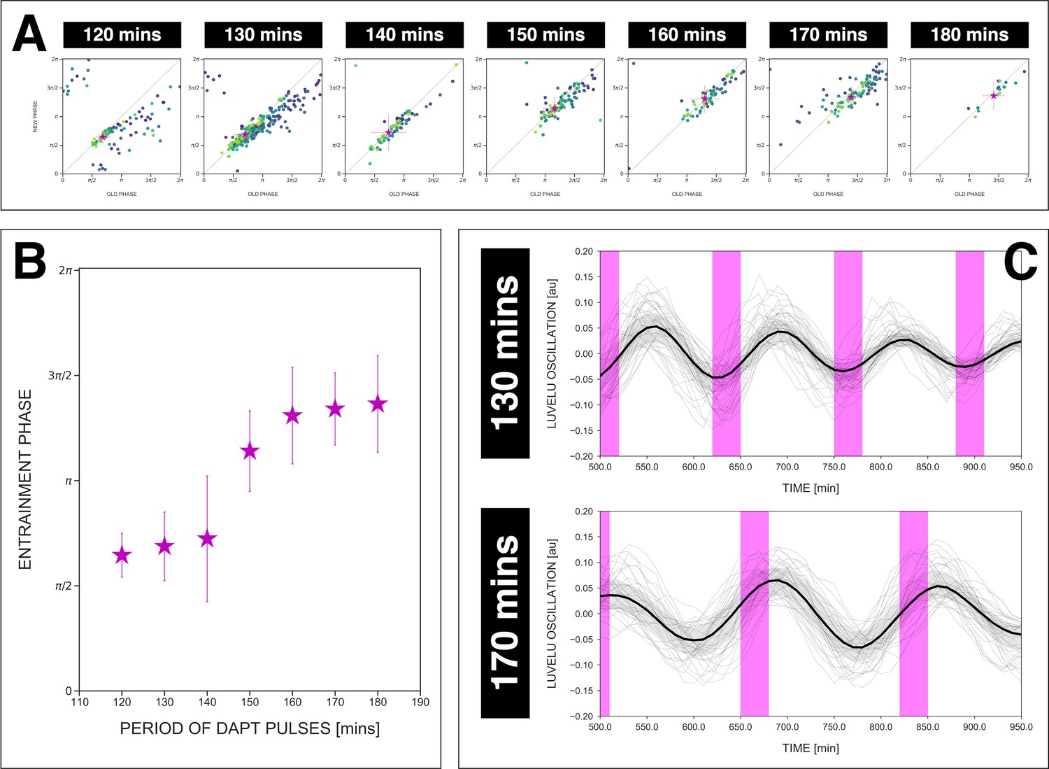
The entrainment phase varies according to zeitgeber period within a range of .
(A) Stroboscopic maps for different periods of DAPT pulses (i.e. zeitgeber periods) placed next to each other. In these maps, only samples that were phase-locked by the end of the experiment are considered (for 120 min: n=13/14 and N=3/3, for 130 min: n=38/39 and N=10/10, for 140 min: n=10/15 and N=3/3, for 150 min: n=16/17 and N=4/4, for 160 min: n=11/15 and N=3/3, for 170 min: n=28/34 and N=8/8, for 180 min: n=4/6 and N=1/1). Here, a sample was considered phase-locked if the difference between its phase at the time of the final drug pulse considered and its phase one drug pulse before is less than . The localized region close to the diagonal in each map marks the entrainment phase () for that zeitgeber period. This is highlighted with a magenta star, which corresponds to the centroid . The centroid was calculated from the vectorial average of the phases of the samples at the end of the experiment, where xc = vectorial average of old phase, yc = vectorial average of new phase. The spread of the points in the region is reported in terms of the circular standard deviation (, where is the first Kuramoto order parameter). The zeitgeber period is indicated above the maps. Colors mark progression in time, from purple to yellow. Stroboscopic maps of all samples and their respective controls are shown in Figure 7—figure supplement 1. Drug concentration and drug pulse duration were kept constant between experiments at 2 µM and 30 min/cycle, respectively. Phase 0 is defined as the peak of the oscillation. (B) Entrainment phase () at different zeitgeber periods, each calculated from the vectorial average of the phases of phase-locked samples at the time corresponding to last considered DAPT pulse. The spread of between samples is reported in terms of the circular standard deviation (, where is the first Kuramoto order parameter). (C) Detrended (via sinc filter detrending) timeseries of the segmentation clock in 2D-assays entrained to either 130 or 170 min periodic pulses of 2 µM DAPT, zoomed in from 500 to 950 min. Periodic pulses are indicated as magenta bars and the timeseries of each sample (for 130 min: n=39 and N=10, for 170 min: n=34 and N=8) is marked with a dashed line. The median of the oscillations is represented here as a solid line, while the gray shaded area denotes the interquartile range. The detrended timeseries for the 130 and 170 min conditions are the same as the detrended timeseries for the 2 µM condition in Figure 4—figure supplement 1A and Figure 4A, respectively. The full detrended timeseries for the 170 min condition can be seen in Figure 3A.
Figure 7—figure supplement 1
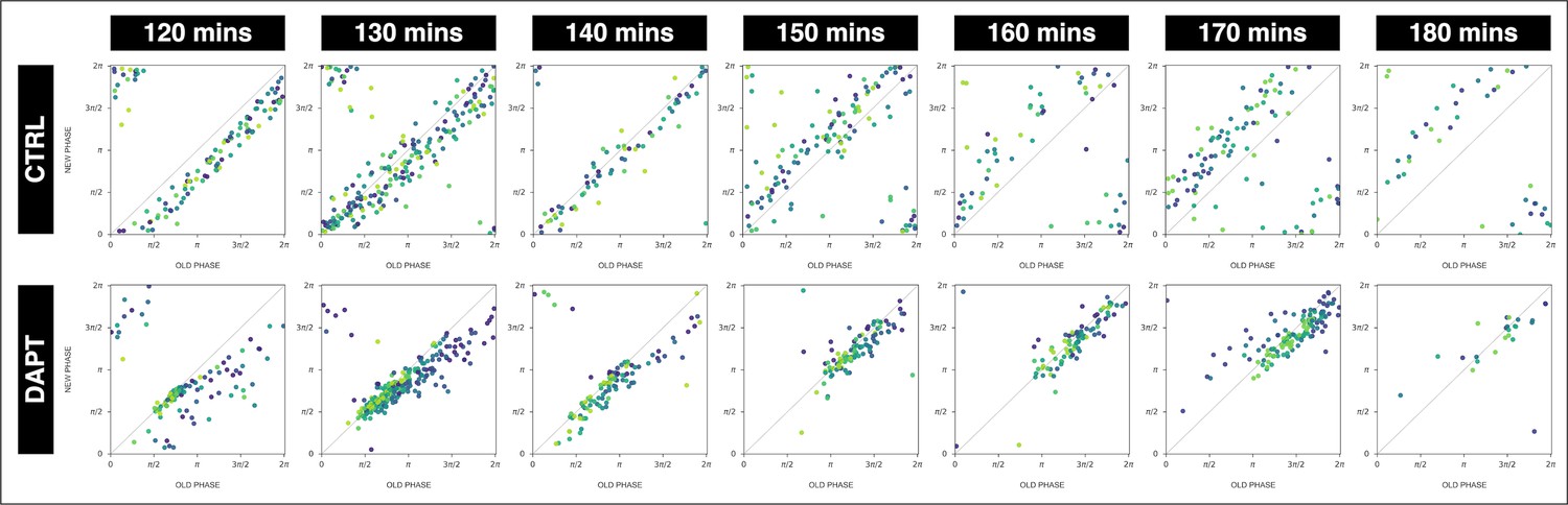
Stable phase relationship with the DAPT pulses.
The segmentation clock establishes a stable phase relationship with the periodic DAPT pulses. Stroboscopic maps summarizing phase dynamics when the segmentation clock was subjected to periodic pulses of 2 µM DAPT (or DMSO for controls). The period of the DAPT (or DMSO) pulses is specified. Colors mark progression in time, from purple to yellow. 120 min: (CTRL: n=14 and N=3) and (DAPT: n=14 and N=3), 130 min: (CTRL: n=30 and N=8) and (DAPT: n=39 and N=10), 140 min: (CTRL: n=10 and N=3) and (DAPT: n=15 and N=3), 150 min: (CTRL: n=20 and N=4) and (DAPT: n=17 and N=4), 160 min: (CTRL: n=10 and N=3) and (DAPT: n=15 and N=3), 170 min: (CTRL: n=24 and N=7) and (DAPT: n=34 and N=8), 180 min: (CTRL: n=10 and N=2) and (DAPT: n=6 and N=1).
Figure 7—figure supplement 2
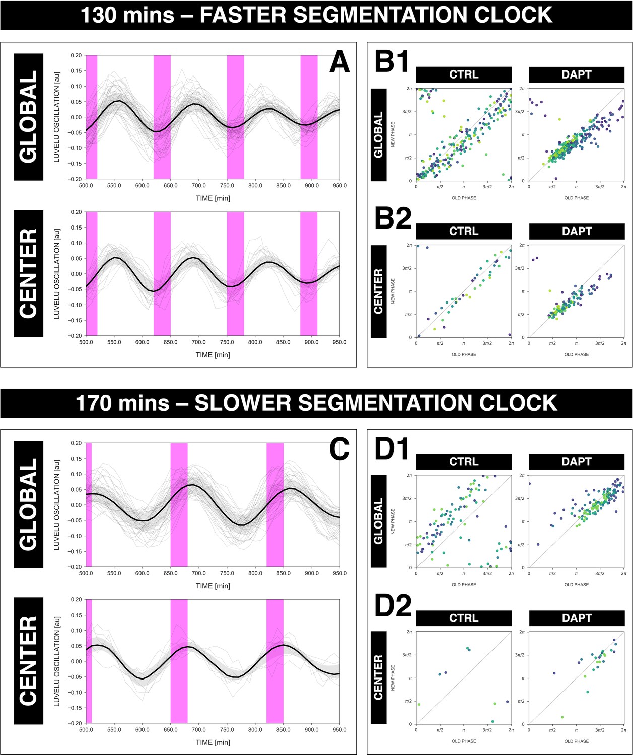
Rhythm of the segmentation clock matches center of 2D-assays.
The rhythm of the segmentation clock matches the rhythm of oscillations in the center of 2D-assays (i.e. the posterior presomitic mesoderm [PSM]) regardless whether the clock is sped up or slowed down. (A) Detrended timeseries (via sinc filter detrending) of either the segmentation clock (global region of interest [ROI], ‘GLOBAL’) or oscillations in the center of 2D-assays (‘CENTER’) entrained to 130 min periodic pulses of 2 µM DAPT, zoomed in from 500 to 950 min. Periodic pulses are indicated as magenta bars and the timeseries of each sample (for GLOBAL: n=39 and N=10, for CENTER: n=15 and N=7) is marked with a dashed line. The median of the oscillations is represented here as a solid line, while the gray shaded area denotes the interquartile range. The plot for GLOBAL is the same as that for the 130 min condition in Figure 7C. (B) Stroboscopic maps of either the segmentation clock GLOBAL, (B1) or oscillations in the center of 2D-assays CENTER, (B2) subjected to 130 min periodic pulses of 2 µM DAPT, with their respective controls (subjected to periodic pulses of DMSO). Colors mark progression in time, from purple to yellow. (C) Detrended timeseries (via sinc filter detrending) of either the segmentation clock (GLOBAL) or oscillations in the center of 2D-assays (CENTER) entrained to 170 min periodic pulses of 2 µM DAPT, zoomed in from 500 to 950 min. Periodic pulses are indicated as magenta bars and the timeseries of each sample (for GLOBAL: n=34 and N=8, for CENTER: n=6 and N=5) is marked with a dashed line. The median of the oscillations is represented here as a solid line, while the gray shaded area denotes the interquartile range. The plot for GLOBAL is the same as that for the 170 min condition in Figure 7C. (D) Stroboscopic maps of either the segmentation clock GLOBAL, (D1) or oscillations in the center of 2D-assays CENTER, (D2) subjected to 170 min periodic pulses of 2 µM DAPT, with their respective controls (subjected to periodic pulses of DMSO). Colors mark progression in time, from purple to yellow.
Figure 7—figure supplement 3
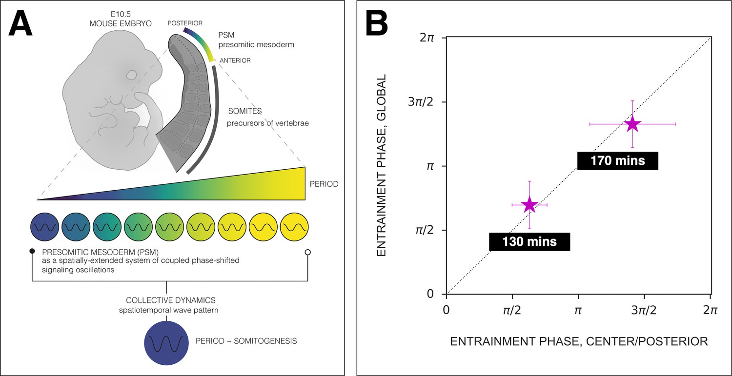
Phase of the segmentation clock matches center of 2D-assays.
The phase of oscillations in the center of 2D-assays (∼posterior presomitic mesoderm [PSM]) matches the phase of the segmentation clock. (A) Scheme of the phase-shifted oscillations along the AP axis of the PSM and its correlation to the segmentation clock. Illustration by Stefano Vianello. (B) Comparison of the phase relationship between the periodic DAPT pulses and either the segmentation clock rhythm (measured in global region of interest [ROI], ‘GLOBAL’) or the rhythm in the center of 2D-assays (equivalent to posterior PSM, ‘CENTER/POSTERIOR’). The entrainment phase was calculated from the vectorial average of the phases of all samples at the time corresponding to the last DAPT pulse considered. The spread of sample phases is reported in terms of the circular standard deviation (, where R is the first Kuramoto order parameter). 130 min: (GLOBAL: n=39 and N=10) and (CENTER: n=15 and N=7), 170 min: (GLOBAL: n=34 and N=8) and (CENTER: n=6 and N=5).
Figure 8 with 4 supplements
Modeling the segmentation clock entrainment response.
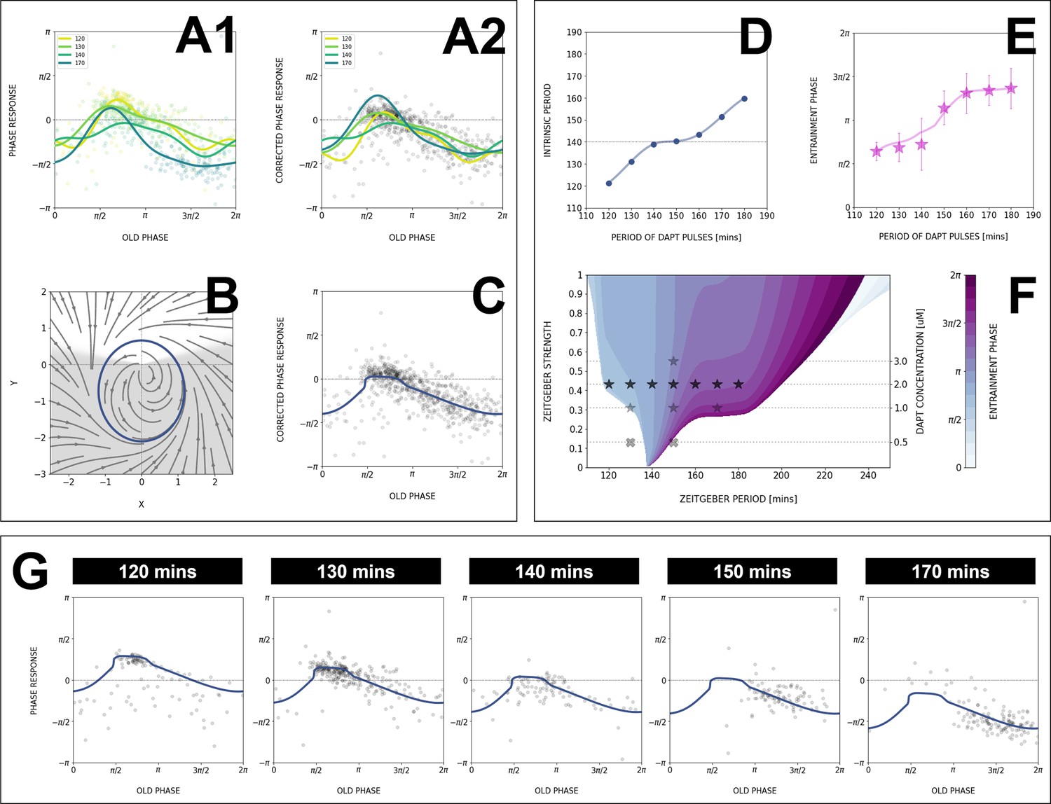
(A) Phase response curve (PRC) from the data for different zeitgeber periods. (1) PRCs calculated at different (points) and Fourier series fitted to them (lines). (2) Original PRCs are shifted vertically to collapse the data points on one curve. (B) Oscillator model, optimized by fitting the vertically shifted PRC. The limit cycle is an ellipse (blue) with eccentricity , the region with speeding up is shaded. (C) Optimized model PRC (line) overlaid to the vertically shifted data points. (D) Modeled intrinsic period as a function of entrainment period . Points were inferred from the PRCs data in A1 by matching the detuning and entrainment phase , the function was interpolated with cubic splines. (E) Entrainment phase from the model with changing intrinsic period (line) agrees with the experimental data (points and error bars). Experimental data are the same as those in Figure 7B. (F) Arnold tongue and isophases calculated with the model. Stars correspond to experimental data with observed entrainment, in agreement with data for different DAPT concentrations (Figure 8—figure supplement 4A). Black stars represent the experiments used for optimizing the model. Crosses correspond to experimental conditions with no entrainment. (G) Fit of the model (solid lines) overlaid with experimental phase differences (dots) at different periods .
Figure 8—figure supplement 1
The segmentation clock keeps its adjusted rhythm a few cycles after release from the zeitgeber.
The segmentation clock keeps its adjusted rhythm even a few cycles after release from DAPT pulses.
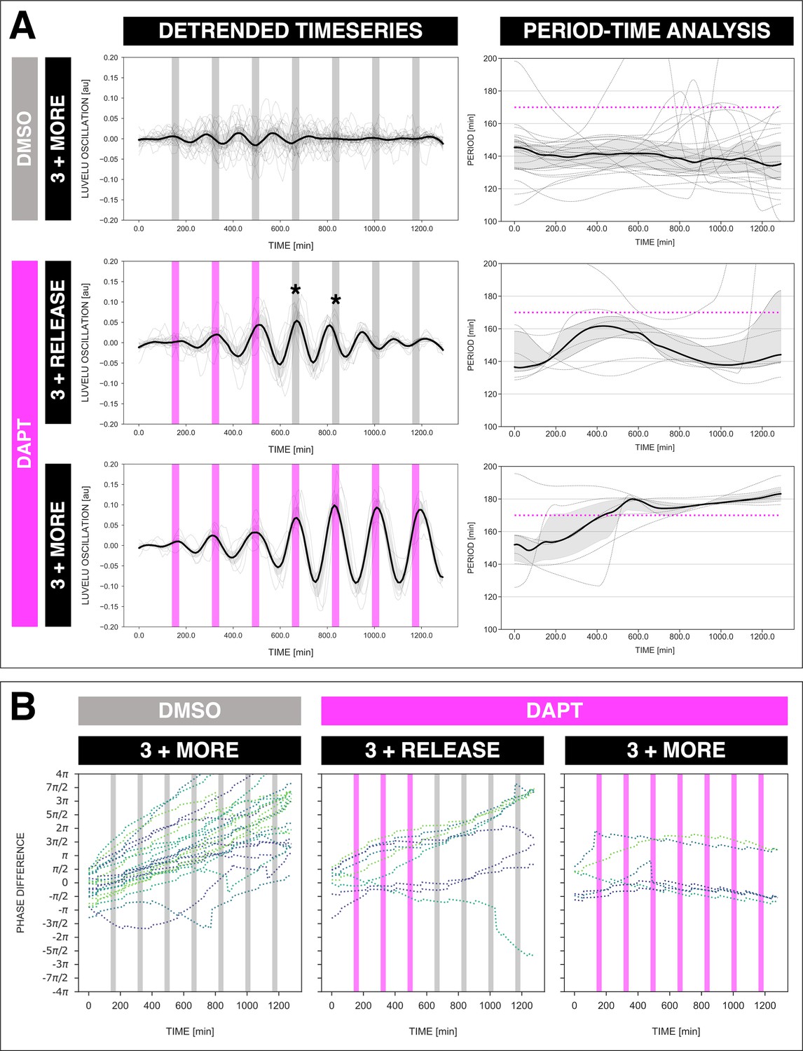
(A) Left: Detrended (via sinc filter detrending) timeseries of the segmentation clock in 2D-assays subjected to 170 min periodic pulses of DMSO (gray bars) and/or 2 µM DAPT (magenta bars). The timeseries of each sample (for continuous DMSO pulses: n=24 and N=7, for three DAPT pulses and then release: n=9 and N=2, for continuous DAPT pulses: n=6 and N=2) is marked with a dashed line. The median of the oscillations is represented here as a solid line, while the gray shaded area denotes the interquartile range. Right: Period evolution during entrainment, obtained from wavelet analysis. The period evolution for each sample and the median of the periods are represented here as a dashed line and a solid line, respectively. The gray shaded area corresponds to the interquartile range. Magenta dashed line marks . Data for the continuous DMSO pulses are the same as the controls in Figure 3A–B. (B) Phase difference between the segmentation clock and the drug pulses. Note that a phase of −/2 is equivalent to a phase of 3π/2, and a phase of 0 is equivalent to a phase of 2π. Periodic pulses of DMSO and 2 µM DAPT are indicated as gray bars and as magenta bars, respectively. Each sample within each condition is marked with different colors.
Figure 8—figure supplement 2
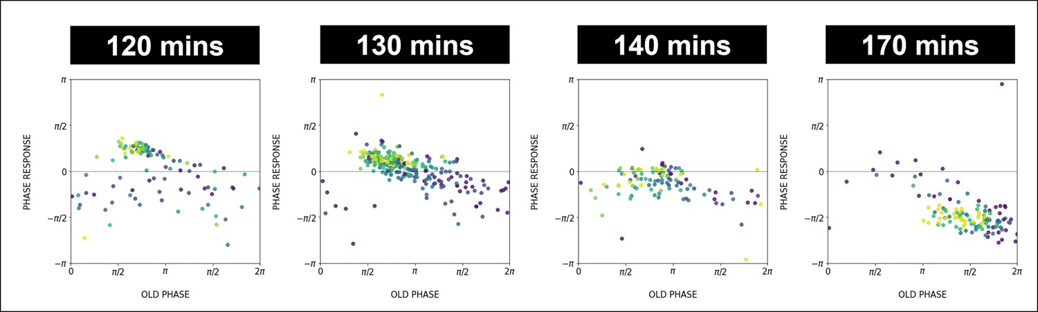
Phase response as a function of time.
We use the color code for pulse number similar to Figure 6 (from purple for early pulses to yellow for later pulses). In the phase response curve (PRC) from the 120 min (170 min) experiment later data points are located higher (lower) than earlier data points, consistent with the change of the intrinsic period of oscillations during entrainment. The adjustment of the intrinsic period decreases the detuning, causing the vertical shift of the phase response curve.
Figure 8—figure supplement 3
The model captures phase response curve (PRC)/phase transition curve (PTC), stroboscopic maps, and entrainment phase.
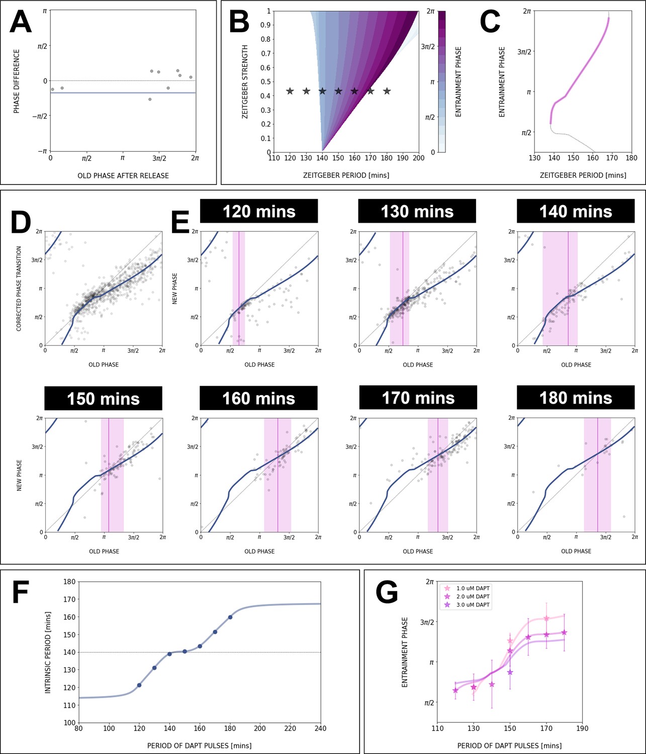
Data for the PRC/PTC, stroboscopic maps, and entrainment phase can be fully captured with our model and changing intrinsic period.
(A) Stroboscopic map data from release experiments allows to estimate the intrinsic oscillation period during entrainment. With min and min, the phase difference between the end and the beginning of the first full cycle with no perturbations is on average 0 (). The data points are from different release experiments with min. If the natural period of 140 min is used, the average phase difference is (solid line). (B, C) Constant intrinsic period is not consistent with experimental data: (B) The Arnold tongue, computed using our model and min, is much narrower than the experimental entrainment range. Stars correspond to experimental conditions (, ) where entrainment was observed. (C) Entrainment phase numerically computed with the optimized PRC from Figure 8C, assuming constant 140 min (which also corresponds to a cross-section of the isophases in B). Clearly, the slope of the curve is much higher than in the data. For comparison, we also plot the Figure 8C PRC rotated by , showing perfect overlap. (D) PTC of the optimized model (equivalent to the PRC shown in Figure 8C). (E) Using the PTC from D, we fit the stroboscopic maps data for all periods by choosing the ) that gives the right detuning. The narrow magenta lines indicate the entrainment phase, the fixed point of each fitted stroboscopic map. The shaded magenta regions show the experimental range for entrainment phase. (F) Extrapolation of the intrinsic oscillator period as a function of zeitgeber period . (G) Cross-sections of the isophases in Figure 8F, calculated with the model and the extrapolated curve for , give excellent agreement with the entrainment phase data for different concentrations of DAPT.
Figure 8—figure supplement 4
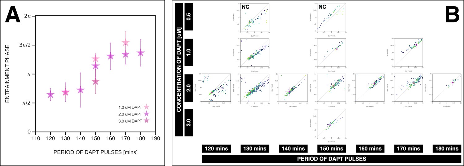
Zeitgeber period and strength affect the entrainment phase.
Zeitgeber period and zeitgeber strength affect the entrainment phase of the segmentation clock. (A) Entrainment phase at different periods of DAPT pulses (i.e. zeitgeber period) and different drug concentrations (i.e. zeitgeber strength). Entrainment phase () was calculated from the vectorial average of the phases of phase-locked samples at the time corresponding to last considered DAPT pulse. A sample was considered phase-locked if the difference between its phase at the time of the final drug pulse considered and its phase one drug pulse before is less than – for 120 min: (2 µM: n=13/14 and N=3/3), for 130 min: (1 µM: n=17/20 and N=4/4), (2 µM: n=38/39 and N=10/10), for 140 min: (2 µM: n=10/15 and N=3/3), for 150 min: (1 µM: n=3/4 and N=1/1), (2 µM: n=16/17 and N=4/4), (3 µM: n=5/5 and N=1/1), for 160 min: (2 µM: n=11/15 and N=3/3), for 170 min: (1 µM: n=12/18 and N=4/5), (2 µM: n=28/34 and N=8/8), for 180 min: (2 µM: n=4/6 and N=1/1). The spread of between samples is reported in terms of the circular standard deviation (, where is the first Kuramoto order parameter). Colors mark concentration of DAPT. Drug pulse duration was kept constant at 30 min/cycle. (B) Stroboscopic maps for different values of zeitgeber period and zeitgeber strength placed next to each other. The localized region close to the diagonal in each map marks for that condition. This is highlighted with a magenta star, which corresponds to the centroid of the said region. The centroid was calculated from the vectorial average of the phases of phase-locked samples at the end of the experiment, where xc = vectorial average of old phase, yc = vectorial average of new phase. The spread of the points in the region is reported in terms of the circular standard deviation (, where is the first Kuramoto order parameter). The period of the DAPT pulses and the concentration of DAPT are indicated. Colors mark progression in time, from purple to yellow. NC means not considered (in plotting A) because no/small fraction of samples was phase-locked – for 0.5 µM 130 min: n=4/9 and N=2/2, for 0.5 µM 150 min: n=0/6 and N=0/1. Stroboscopic maps for these NC conditions include all samples, unlike the other conditions where only phase-locked samples are plotted. Data for 2 µM condition is the same as that in Figure 7A–B.
Appendix 1—figure 1 with 5 supplements
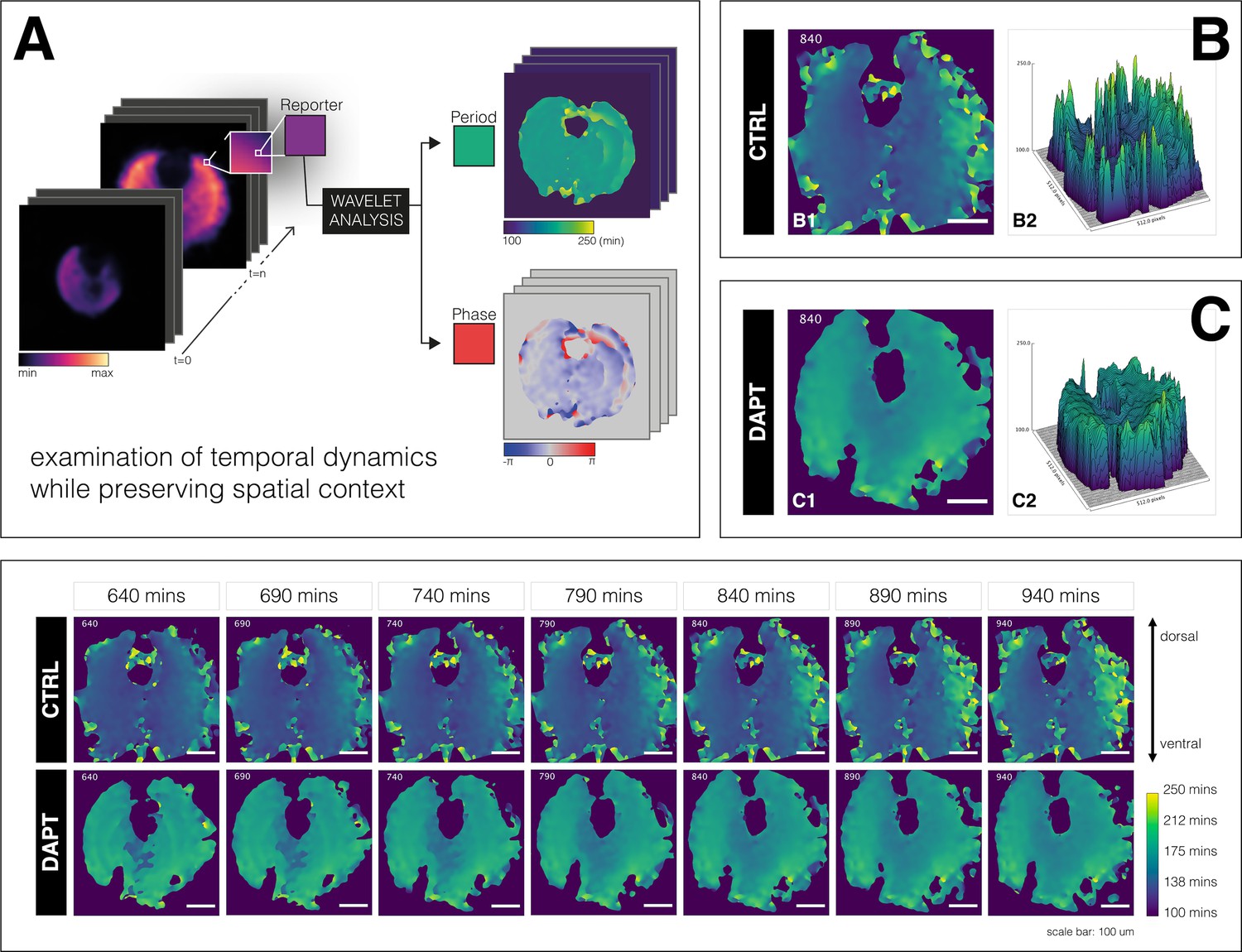
A spatial period gradient emerges in the tissue even upon entrainment of the segmentation clock.
Left: Schematic of pipeline to generate period and phase movies using pixel-by-pixel wavelet analysis (A). Illustration by Stefano Vianello. Right: Snapshot of period wavelet movie of control subjected to 170 min periodic pulses of DMSO (B) or entrained sample subjected to 170 min periodic pulses of 2 µM DAPT (C), taken at 840 min after the start of experiment. Period is either shown using heatmap (B1,C1) or as a surface plot (B2,C2). Bottom: Snapshots of period wavelet movie of samples in (B) and (C) at different time points. Time is indicated as minutes elapsed from the start of the experiment. Sample is rotated so that the dorsal side is up. Timelapse of period wavelet movies and corresponding surface plots are available at https://youtu.be/3Y53OhXacKI.
Appendix 1—figure 1—video 1
Period gradient of LuVeLu in E10.5 2D-assay subjected to 170 min periodic pulses of 2 µM DAPT (or DMSO for control) available at https://youtu.be/3Y53OhXacKI.
Appendix 1—figure 1—video 2
E10.5 2D-assay, expressing LuVeLu, subjected to 170 min periodic pulses of DMSO control, with corresponding period and phase wavelet movies, available at https://github.com/PGLSanchez/EMBL-files/blob/master/MOVIES/SO_2.0D_170mins_CTRL.avi.
Appendix 1—figure 1—video 3
E10.5 2D-assay, expressing LuVeLu, subjected to 170 min periodic pulses of 2 µM DAPT, with corresponding period and phase wavelet movies, available at https://github.com/PGLSanchez/EMBL-files/blob/master/MOVIES/SO_2.0D_170mins_DAPT.avi.
Appendix 1—figure 1—video 4
E10.5 2D-assay, expressing LuVeLu, subjected to 130 min periodic pulses of DMSO control, with corresponding period and phase wavelet movies, available at https://github.com/PGLSanchez/EMBL-files/blob/master/MOVIES/SO_2.0D_130mins_CTRL.avi.
Appendix 1—figure 1—video 5
E10.5 2D-assay, expressing LuVeLu, subjected to 130 min periodic pulses of 2 µM DAPT, with corresponding period and phase wavelet movies, available at https://github.com/PGLSanchez/EMBL-files/blob/master/MOVIES/SO_2.0D_130mins_DAPT.avi.
Appendix 1—figure 2
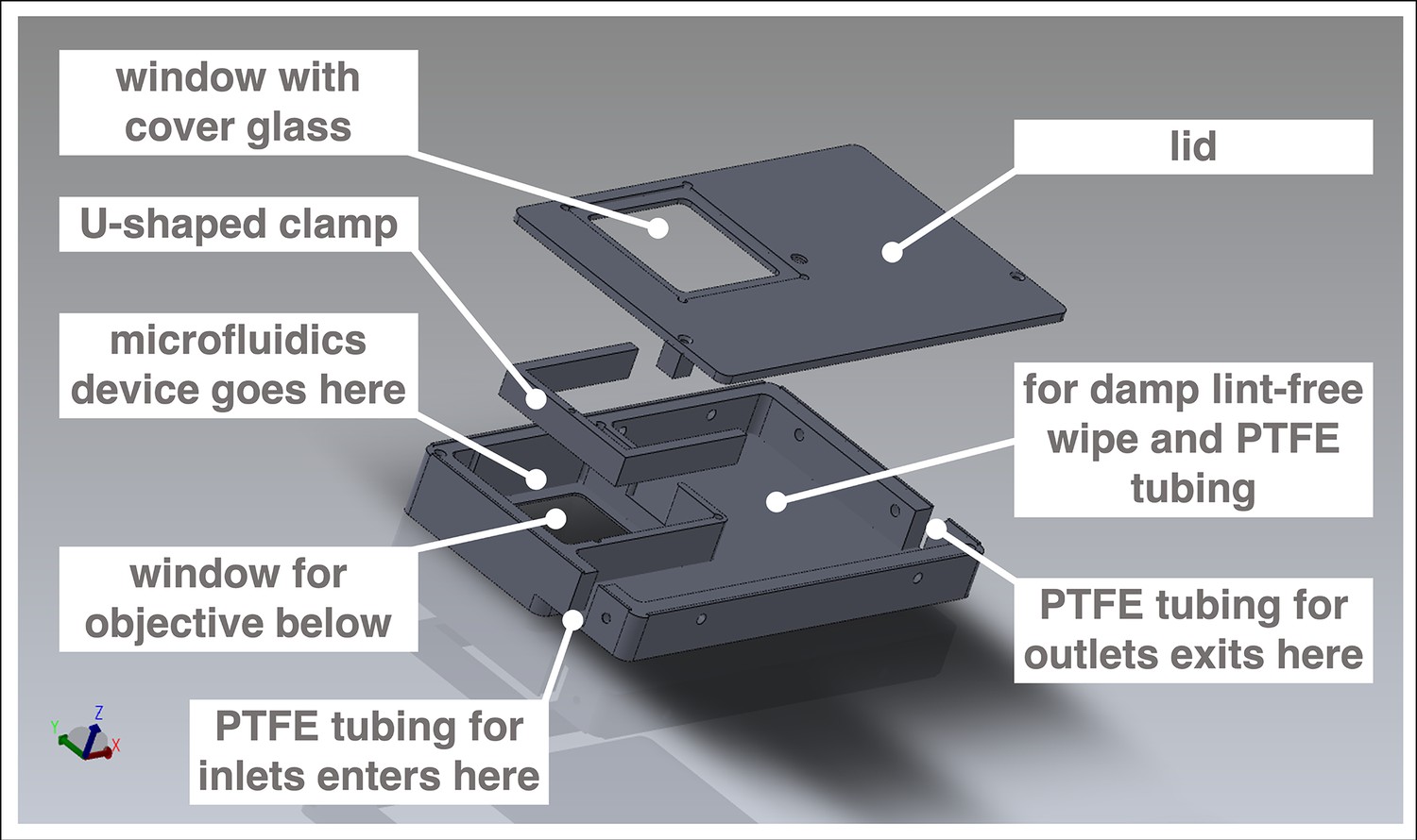
Customized box to mount microfluidics device on microscope for simultaneous culture, entrainment, and live imaging.
Computer-aided design (CAD) of metal box customized to hold a microfluidics device bonded to a 70 mm × 70 mm cover glass. The box fits the stage of an LSM 780 laser-scanning microscope (Carl Zeiss Microscopy). Design by Katharina Sonnen, the EMBL Mechanical Design Office, and the EMBL Mechanical Workshop.
Appendix 1—figure 3
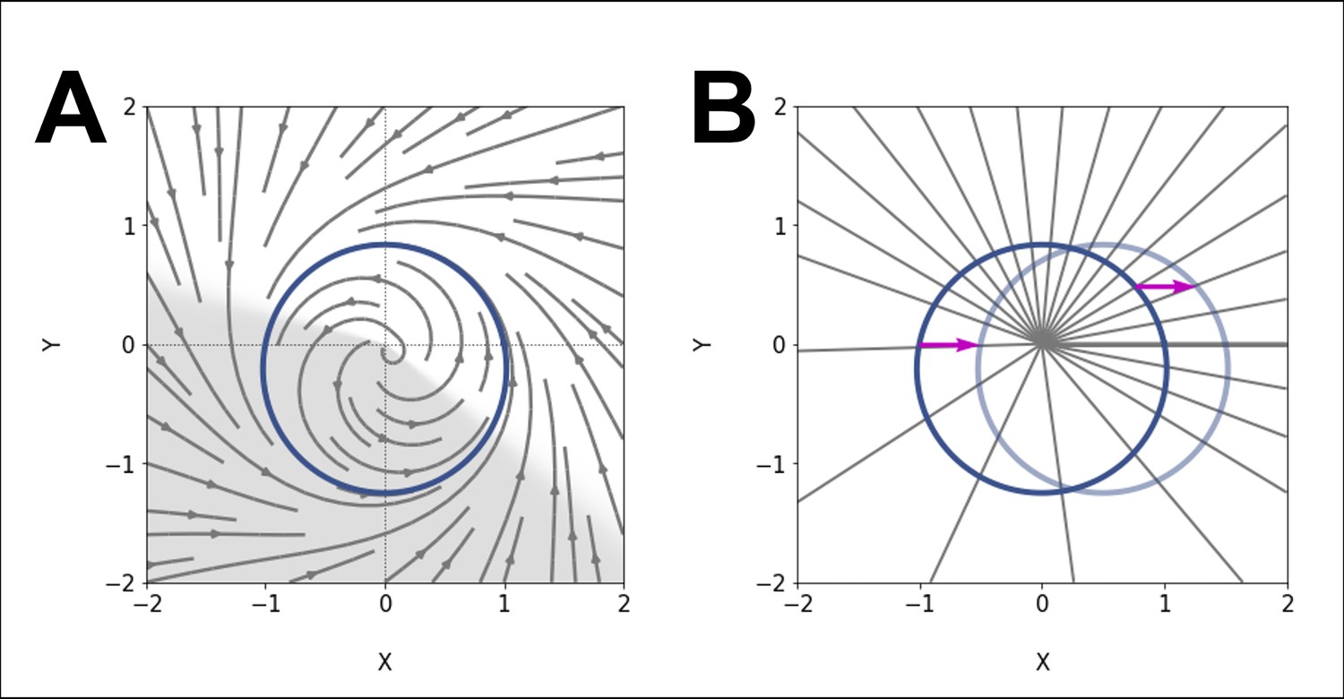
ERICA model.
(A) Our model consists of an elliptic limit cycle (blue) with increased angular velocity in one sector (shaded region). (B) The effect of such acceleration is to change the spacing of isochrons (radial lines). We compute the phase response curve (PRC) of the model by introducing a perturbation (arrow) at points on the limit cycle and looking at the starting and ending isochrons.
Appendix 1—figure 4
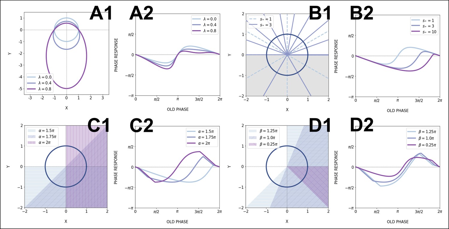
Effects of model parameters on the phase response curve (PRC).
(A) Effect of eccentricity : (A1) Increasing makes the limit cycle more elongated, while keeping the upper focus at the origin. (A2) The positive part of the PRC is then flattened; for all PRCs here (no acceleration). (B) Effect of speeding up : (B1) When is increased, the spacing between isochrons in the sped up region increases, so this region contains less and less isochrons. Shown here is the case when the acceleration happens in the lower half-plane (, ), which is shaded in gray. (B2) The effect on the PRC is to shrink the portion where the oscillator is sped up, thus emphasizing the other part of the curve. Here, . (C, D) Effects of the sped up sector parameters : the location and width of the sector determine which parts of the PRC get rescaled. (C1) The shaded regions are sectors with different values of and . (C2) The corresponding PRCs with,.. (D1) Sped up sectors located at with different widths . (D2) The corresponding PRCs for the case .. All PRCs in this figure were computed with perturbation amplitude .
Author response image 1

Author response image 2
Tzeit = 120.
Author response image 3

Tzeit = 140.
Author response image 4
Tzeit = 150.
Author response image 5
Tzeit = 160.
Author response image 6

Tzeit = 180.
Author response image 7
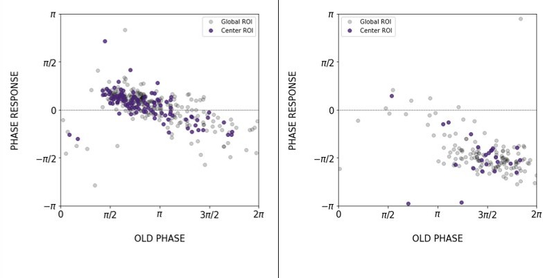
Comparison of the PRC obtained with global ROI and center ROI, T_zeit = 130 min (left) and 170 min (right).
Tables
Table 1
Summary statistics on period-locking of the segmentation clock in E10.5 2D-assays to periodic pulses of 2 µM DAPT.
This table summarizes the median, 95% confidence interval (CI) of the median, mean, standard deviation (SD), and standard error of the mean (SEM) of the segmentation clock in 2D-assays subjected to periodic pulses of 2 µM DAPT. These summary statistics were determined using PlotsOfData (Postma and Goedhart, 2019). A plot of these data is shown in Figure 3D.
| Pulse period | n | N | Median, min | 95% CI of median, min | Mean, min | SD, min | SEM, min |
|---|---|---|---|---|---|---|---|
| 120 min | 14 | 3 | 127.36 | 123.16–148.03 | 139.39 | 22.28 | 6.18 |
| 130 min | 39 | 10 | 133.44 | 132.21–135.97 | 134.75 | 4.56 | 0.74 |
| 140 min | 15 | 3 | 147.68 | 146.10–153.02 | 150.00 | 7.42 | 1.98 |
| 150 min | 17 | 4 | 155.14 | 154.33–160.74 | 158.18 | 7.77 | 1.94 |
| 160 min | 15 | 3 | 167.09 | 166.16–169.84 | 167.33 | 5.28 | 1.41 |
| 170 min | 34 | 8 | 176.14 | 173.06–181.20 | 175.56 | 8.52 | 1.48 |
| 180 min | 6 | 1 | 184.43 | 164.54–194.21 | 181.06 | 17.88 | 8.00 |
Appendix 1—key resources table
| Reagent type (species) or resource | Designation | Source or reference | Identifiers | Additional information |
|---|---|---|---|---|
| Genetic reagent (Mus musculus) | LuVeLu | Aulehla et al. | DOI:10.1038/ncb1679 | |
| Genetic reagent (Mus musculus) | Mesp2-GFP | Morimoto et al. | DOI:10.1016/j.ydbio.2006.08.043 | |
| Genetic reagent (Mus musculus) | Axin2-linker- Achilles | This work | see Materials and methods > Mouse lines | |
| Chemical compound, drug | Bovine serum albumin (BSA) | Equitech-Bio | BAC62 | |
| Chemical compound, drug | DMEM/F12 | Cell Culture Technologies | Customized | No glucose, glutamate, L-glutamine, and phenol red |
| Chemical compound, drug | 1 M HEPES | Gibco | 15630-106 | |
| Chemical compound, drug | 10,000 U/mL PenStrep | Gibco | 15140-122 | |
| Chemical compound, drug | 45% glucose | Sigma | G8769 | |
| Chemical compound, drug | 200 mM L-glutamine | Gibco | 25030-081 | |
| Chemical compound, drug | Fibronectin | Sigma-Aldrich | F1141 | |
| Chemical compound, drug | Cascade Blue | Invitrogen | C-3239 | |
| Chemical compound, drug | DMSO | Sigma-Aldrich | D8418 | |
| Chemical compound, drug | DAPT | Sigma-Aldrich | D5942-5MG | Stock concentration in DMSO: 10 mM |
| Commercial assay, kit | SYLGARD 184 silicone kit | Dow | 1673921 | 9:1 (w/w) elastomer base: curing agent |
| Software, algorithm | Microscopy Pipeline Constructor (MyPiC) | Politi et al., 2018 | DOI:10.1038/nprot.2018.040 | https://github.com/manerotoni/mypic/ |
| Software, algorithm | Fiji | Schindelin et al. | DOI:10.1038/nmeth.2019 | |
| Software, algorithm | Matplotlib | Hunter | DOI:10.1109/MCSE.2007.55 | |
| Software, algorithm | NumPy | van der Walt et al. | DOI:10.1109/MCSE.2011.37 | |
| Software, algorithm | pandas | McKinney | DOI:10.25080/Majora-92bf1922-00a | |
| Software, algorithm | scikit-image | van der Walt et al. | DOI:10.7717/peerj.45310.7717/peerj.453 | |
| Software, algorithm | SciPy | Virtanen et al. | DOI:10.1038/s41592-019-0686-2 | |
| Software, algorithm | seaborn | Waskom et al. | DOI:10.5281/zenodo.12710 | |
| Software, algorithm | PlotTwist | Goedhart | DOI:10.1371/journal.pbio.3000581 | https://huygens.science.uva.nl/PlotTwist/ |
| Software, algorithm | PlotsOfData | Postma and Goedhart | DOI:10.1371/journal.pbio.3000202 | https://huygens.science.uva.nl/PlotsOfData/ |
| Software, algorithm | PlotsOfDifferences | Goedhart | DOI:10.1101/578575 | https://huygens.science.uva.nl/PlotsOfDifferences/ |
| Software, algorithm | pyBOAT | Mönke, 2020a | DOI:10.1101/2020.04.29.067744 | https://github.com/tensionhead/pyBOAT/ |
| Software, algorithm | Spatial pyBOAT (SpyBOAT) | Mönke, 2020b | https://github.com/tensionhead/SpyBOAT/ | |
| Software, algorithm | Entrainment Analysis Jupyter notebook | This work, Sanchez, 2022 | EntrainmentAnalysis in https://github.com/PGLSanchez/EMBL_OscillationsAnalysis/ | |
| Other | Cover glass | Marienfeld | 0107999 098 | 70 mm × 70 mm, 1.5H, see Materials and methods > Preparations for microfluidics- based entrainment of 2D-assays |
| Other | PTFE tubing | APT | AWG24T | Inner diameter: 0.6 mm, see Materials and methods > Preparations for microfluidics- based entrainment of 2D-assays |
| Other | Syringe needle | BD Microlance 3 | 300900 | 22G×1.25" – Nr. 12, see Materials and methods > Preparations for microfluidics- based entrainment of 2D-assays |
| Other | 3 mL syringe | BD Luer-Lok | 309658 | Diameter: 8.66 mm, see Materials and methods > Preparations for microfluidics- based entrainment of 2D-assays |
| Other | 10 mL syringe | BD Luer-Lok | 300912 | Diameter: 14.5 mm, see Materials and methods > Preparations for microfluidics- based entrainment of 2D-assays |
| Other | Programmable pump | World Precision Instruments | AL-400 | see Materials and methods > Setting up automated pumping |
| Other | LSM 780 laser-scanning microscope | Carl Zeiss Microscopy | see Materials and methods > Confocal microscopy |
Appendix 1—table 1
Recipe for media preparation.
Formulations specified here are for the preparation of approximately 50 mL of medium. Special DMEM/F12* used in these media does not contain glucose, L-glutamine, sodium pyruvate, and phenol red. Culture medium is filter sterilized after preparation.
| Component | Dissection medium | Culture medium |
|---|---|---|
| BSA (Equitech-Bio, BAC62) | 0.5 g | 0.02 g |
| DMEM/F12* (Cell Culture Technologies) | 50 mL | 50 mL |
| 1 M HEPES (Gibco, 15630-106) | 1 mL | – |
| 10,000 U/mL PenStrep (Gibco, 15140-122) | – | 500 µL |
| 45% Glucose (Sigma, G8769) | 44.4 µL | 44.4 µL |
| 200 mM L-Glutamine (Gibco, 25030-081) | 500 µL | 500 µL |
Appendix 1—table 2
List of PTFE tubing needed for a microfluidics-based entrainment experiment.
For the first two items, a syringe needle is to be inserted inside one end of each tubing. Plugs are made from cut PDMS-filled PTFE tubing, and are used to seal inlets after sample loading. Controls are already taken into account in the specified quantities.
| Item | With needle? | Quantity | Use |
|---|---|---|---|
| 3 m PTFE tubing | Y | 4 | Drug/medium inlet |
| 1 m PTFE tubing | Y | 2 | Outlet |
| 1 cm plug | N | 24 | Sample inlet+unused drug/medium inlet |
Appendix 1—table 3
List of syringe containing drug/medium for a microfluidics-based entrainment experiment.
Formulations specified here are for any drug with final concentration X µM. For recipe to prepare culture medium, please refer to Appendix 1—table 2.
| Component | Syringe A | Syringe B | Syringe C | Syringe D |
|---|---|---|---|---|
| DRUG | CONTROL | MEDIUM | MEDIUM | |
| Drug (10 mM in DMSO) | X µL | – | – | – |
| DMSO (Sigma-Aldrich, D8418) | – | X µL | – | – |
| Cascade Blue (Invitrogen, C-3239) | 2 µL | 2 µL | – | – |
| Culture medium (see Appendix 1—table 2) | Dilute to 10 mL | Dilute to 10 mL | 10 mL | 10 mL |
Appendix 1—table 4
Pumping program of medium for entrainment to 170 min periodic pulses of drug.
| Phase | Function | Rate | Volume | Remark |
|---|---|---|---|---|
| PH:01 | LP:ST | |||
| PH:02 | RATE | 60 µL/hr | 140 µL | Perfuse medium for 140 min |
| PH:03 | LP:ST | |||
| PH:04 | PS:60 | Pause for 60 s | ||
| PH:05 | LP:30 | Loop PH:04 30 times (pause for 30 min=60 s × 30) | ||
| PH:06 | LP:30 | Loop PH:02 to PH:05 30 times (total: 30 periodic pulses) | ||
| PH:07 | STOP |
Appendix 1—table 5
Pumping program of drug/control for entrainment to 170 min periodic pulses of drug.
| Phase | Function | Rate | Volume | Remark |
|---|---|---|---|---|
| PH:01 | LP:ST | |||
| PH:02 | LP:ST | |||
| PH:03 | LP:ST | |||
| PH:04 | PS:60 | Pause for 60 s | ||
| PH:05 | LP:70 | Loop PH:04 70 times (pause for 70 min=60 s × 70) | ||
| PH:06 | LP:02 | Loop PH:04 to PH:05 2 times (pause 140 min=70 mins × 2) | ||
| PH:07 | RATE | 60 µL/hr | 30 µL | Perfuse drug/control for 30 min |
| PH:08 | LP:30 | Loop PH:02 to PH:07 30 times (total: 30 periodic pulses) | ||
| PH:09 | STOP |
Additional files
Download links
A two-part list of links to download the article, or parts of the article, in various formats.
Downloads (link to download the article as PDF)
Open citations (links to open the citations from this article in various online reference manager services)
Cite this article (links to download the citations from this article in formats compatible with various reference manager tools)
Arnold tongue entrainment reveals dynamical principles of the embryonic segmentation clock
eLife 11:e79575.
https://doi.org/10.7554/eLife.79575


