Quantifying dynamic facial expressions under naturalistic conditions
- School of Psychology, College of Engineering, Science and the Environment, University of Newcastle, Australia
- Hunter Medical Research Institute, Australia
- School of Psychological Sciences, University of Western Australia, Australia
- School of Psychiatry, University of New South Wales, Australia
- School of Medicine and Public Health, College of Medicine, Health and Wellbeing, University of Newcastle, Australia
Figures
Figure 1 with 2 supplements
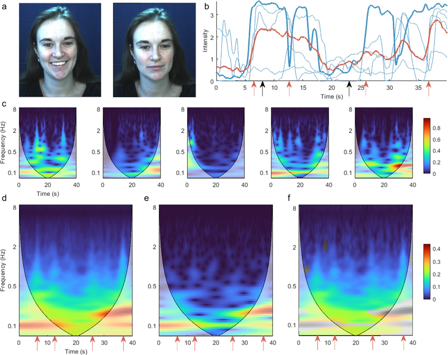
Time-frequency representation of action unit 12 ‘Lip Corner Puller’ during positive valence video stimulus reveals high-frequency dynamics.
(a) Example participant’s facial reactions at two time points, corresponding to high and low activation of action unit 12. (b) Action unit time series for five example participants (blue). Bold line corresponds to the participant shown in panel (a), and black arrows indicate time points corresponding to the representative pictures. The group mean time course across all participants is shown in red. Red arrows indicate funny moments in the stimulus, evoking sudden facial changes in individual participants. These changes are less prominent in the group mean time course. (c) Time-frequency representation for the same five participants, calculated as the amplitude of the continuous wavelet transform. Intuitively, the heatmap colour indicates how much of each frequency is present at each time point. Shading indicates the cone of influence – the region contaminated by edge effects. (d) Mean of all participants’ time-frequency representations. Red arrows correspond to time points with marked high-frequency activity above 1 Hz (e) Time-frequency representation of the group mean time course. (f) Difference between (d) and (e). Non-significant differences (p>0.05) are shown in greyscale. Common colour scale is used for (d–f).
Figure 1—figure supplement 1
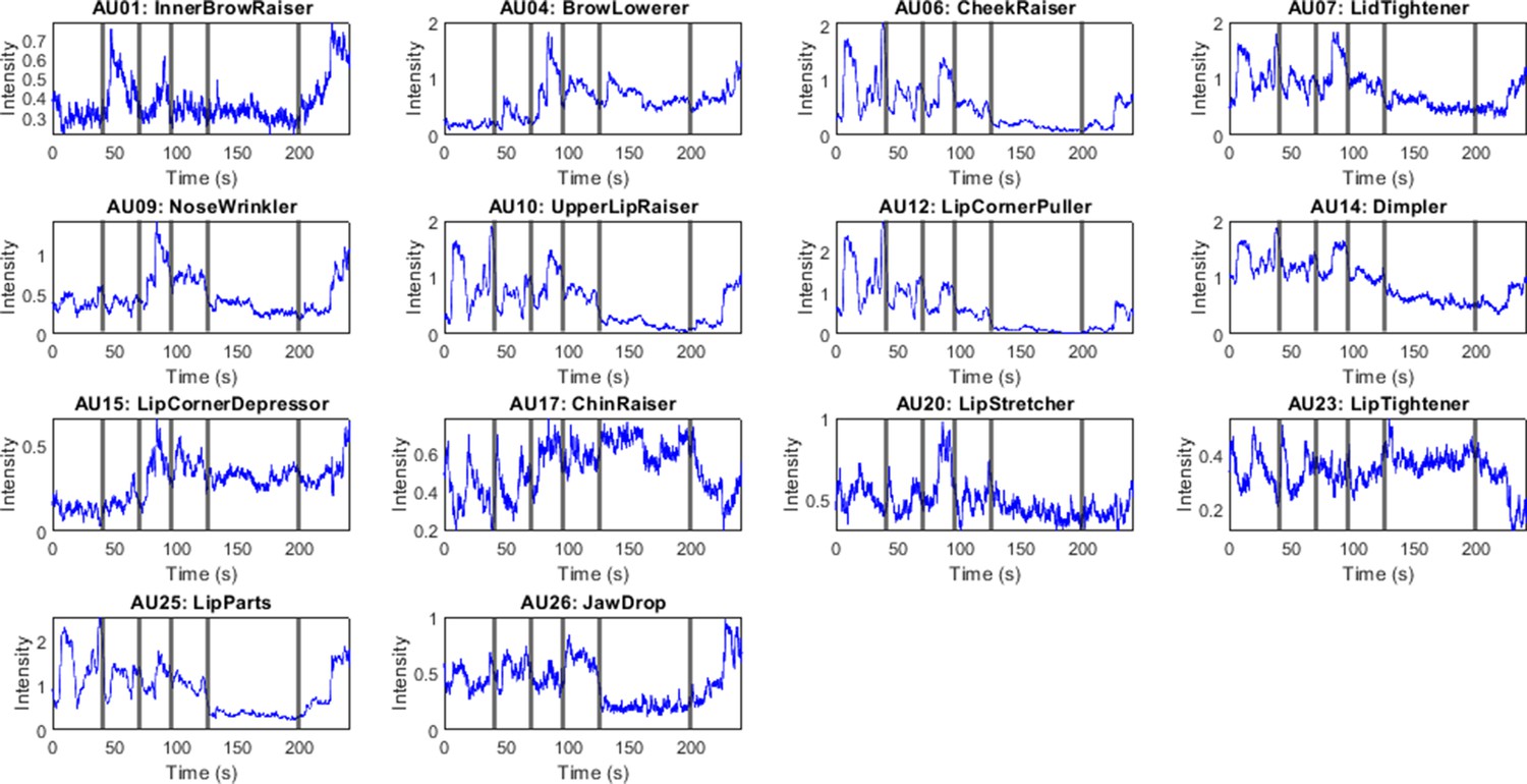
Mean of raw time series, Denver Intensity of Spontaneous Facial Action (DISFA) dataset.
Vertical lines demarcate video clips described in Supplementary file 1.
Figure 1—figure supplement 2
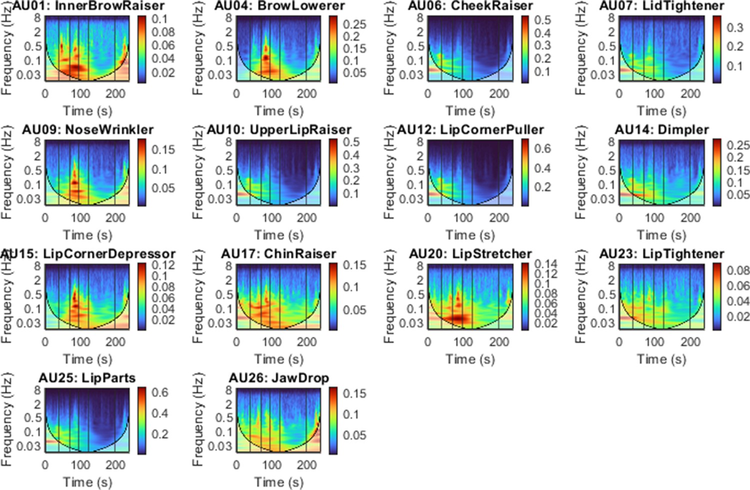
Mean of time-frequency representation across all participants in Denver Intensity of Spontaneous Facial Action (DISFA) dataset.
Shading indicates the cone of influence. Vertical lines demarcate video clips described in Supplementary file 1.
Figure 2
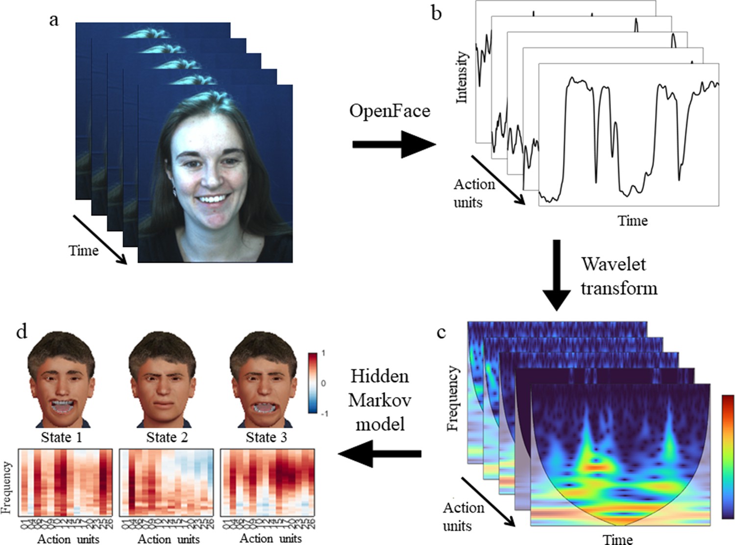
Visual overview of the pipeline.
(a) Participant’s facial responses while viewing a naturalistic stimulus. (b) OpenFace extracts the time series for each action unit. (c) The continuous wavelet transform produces a time-frequency representation of the same data. (d) A hidden Markov model infers dynamic facial states common to all participants. Each state has a unique distribution over action units and frequency bands.
Figure 3 with 20 supplements
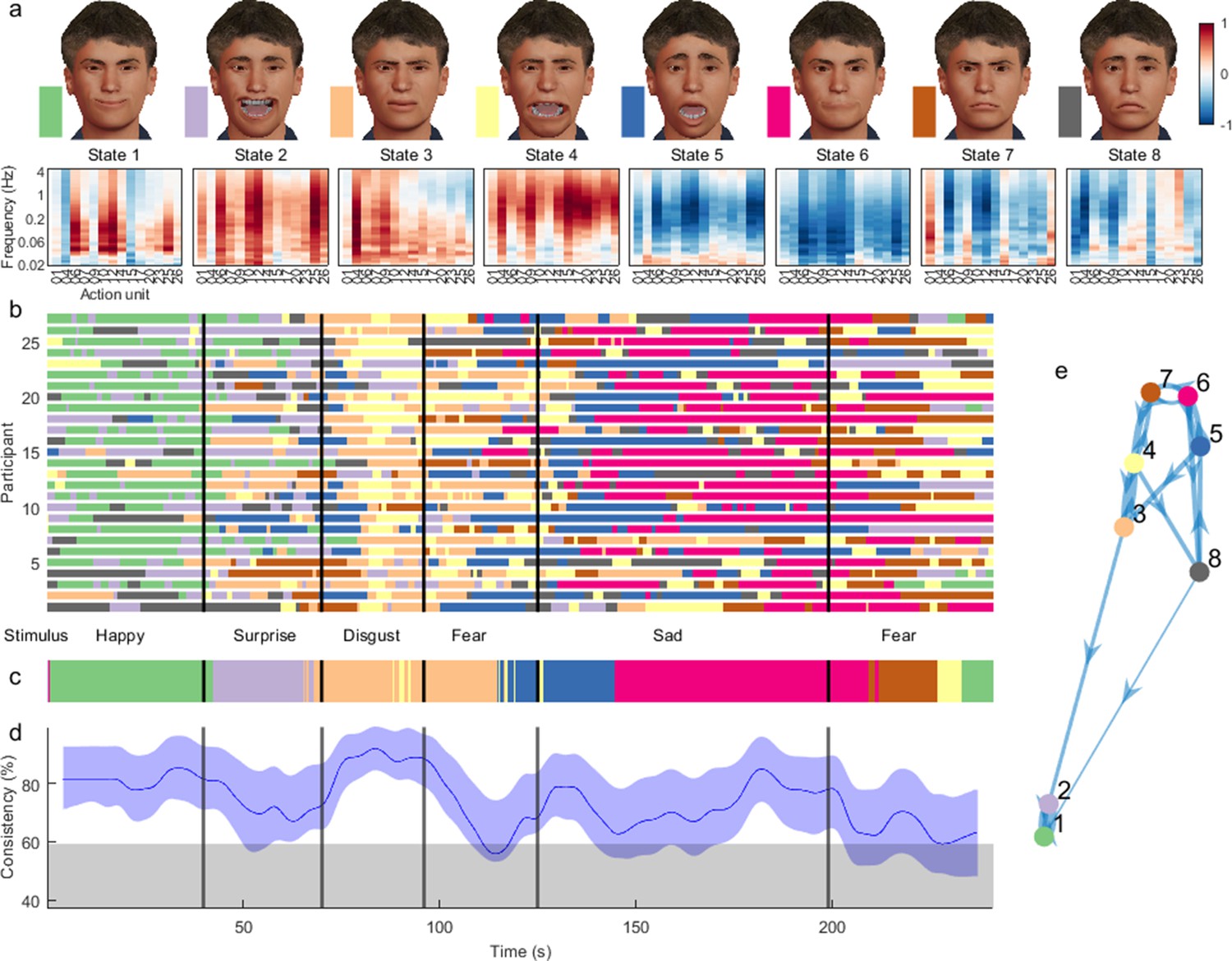
Dynamic facial states inferred from time-frequency representation of Denver Intensity of Spontaneous Facial Action (DISFA) dataset.
(a) Mean of the observation model for each state, showing their mapping onto action units and frequency bands. Avatar faces (top row) for each state show the relative contribution of each action unit, whereas their spectral projection (bottom row) shows their corresponding dynamic content. (b) Sequence of most likely states for each participant at each time point. Vertical lines demarcate transition between stimulus clips with different affective annotations. (c) Most common states across participants, using a 4 s sliding temporal window. (d) Proportion of participants expressing the most common state. Blue shading indicates 5–95% bootstrap confidence bands for the estimate. Grey shading indicates the 95th percentile for the null distribution, estimated using time-shifted surrogate data. (e) Transition probabilities displayed as a weighted graph. Each node corresponds to a state. Arrow thickness indicates the transition probability between states. For visualisation clarity, only the top 20% of transition probabilities are shown. States are positioned according to a force-directed layout where edge length is the inverse of the transition probability.
Figure 3—figure supplement 1
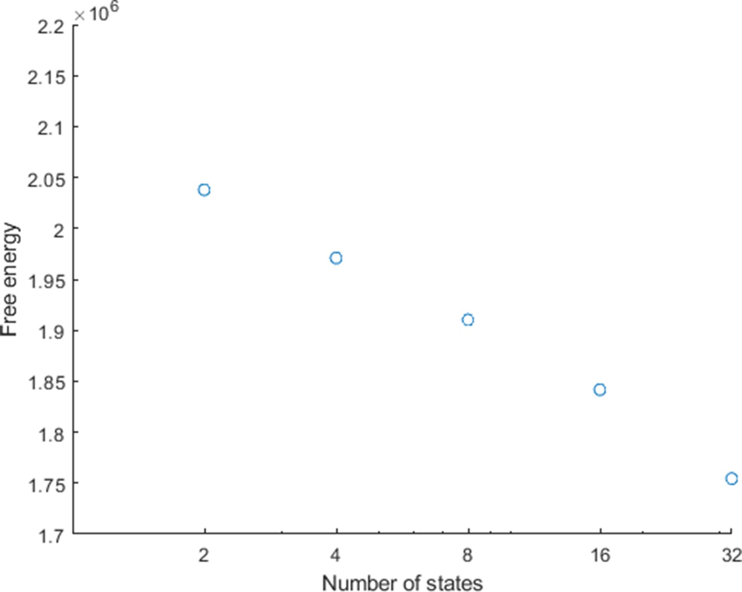
Free energy of the hidden Markov model as a function of number of states.
Free energy continues to decrease as the number of states increases (logarithmic scale).
Figure 3—video 1
Example subject 1 in hidden Markov model (HMM) state 1.
Figure 3—video 2
Example subject 1 in hidden Markov model (HMM) state 2.
Figure 3—video 3
Example subject 1 in hidden Markov model (HMM) state 3.
Figure 3—video 4
Example subject 1 in hidden Markov model (HMM) state 4.
Figure 3—video 5
Example subject 1 in hidden Markov model (HMM) state 5.
Figure 3—video 6
Example subject 1 in hidden Markov model (HMM) state 6.
Figure 3—video 7
Example subject 2 in hidden Markov model (HMM) state 1.
Figure 3—video 8
Example subject 2 in hidden Markov model (HMM) state 3.
Figure 3—video 9
Example subject 2 in hidden Markov model (HMM) state 4.
Figure 3—video 10
Example subject 2 in hidden Markov model (HMM) state 5.
Figure 3—video 11
Example subject 2 in hidden Markov model (HMM) state 6.
Figure 3—video 12
Example subject 2 in hidden Markov model (HMM) state 7.
Figure 3—video 13
Example subject 2 in hidden Markov model (HMM) state 8.
Figure 3—video 14
Example subject 3 in hidden Markov model (HMM) state 1.
Figure 3—video 15
Example subject 3 in hidden Markov model (HMM) state 2.
Figure 3—video 16
Example subject 3 in hidden Markov model (HMM) state 3.
Figure 3—video 17
Example subject 3 in hidden Markov model (HMM) state 4.
Figure 3—video 18
Example subject 3 in hidden Markov model (HMM) state 6.
Figure 3—video 19
Example subject 3 in hidden Markov model (HMM) state 7.
Figure 4 with 3 supplements
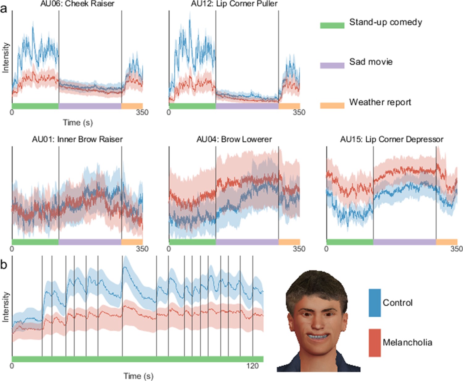
At each time point, mean intensity across participants of facial action unit activation in controls (blue) and melancholia (red).
Shading indicates 5% and 95% confidence bands based on a bootstrap sample (n=1000). (a) Action units commonly implicated in happiness (top row) and sadness (bottom row). Participants watched stand-up comedy, a sad video, and a funny video in sequence. Vertical lines demarcate transitions between video clips. (b) First principal component of action units, shown during stand-up comedy alone. Vertical lines indicate joke annotations. Avatar face shows the relative contribution of each action unit to this component.
Figure 4—figure supplement 1
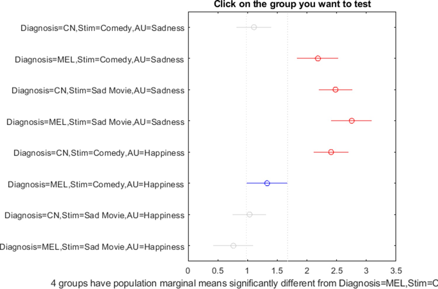
Comedy vs. sad movie.
Post hoc comparison intervals using Tukey’s honestly significant difference criterion (p=0.05).
Figure 4—figure supplement 2
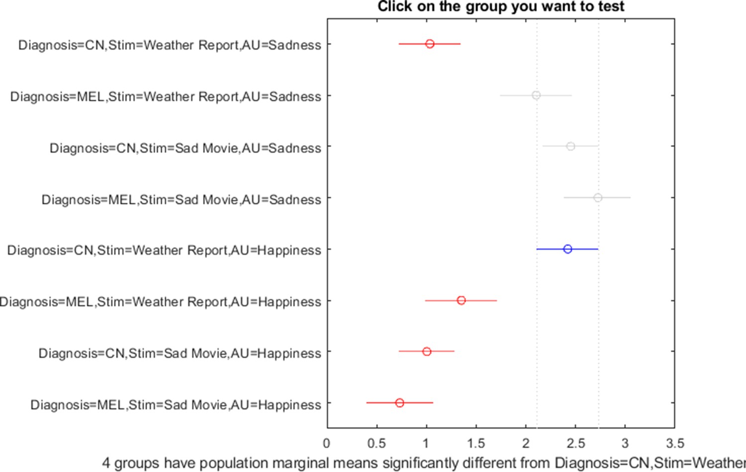
Weather report vs. sad movie.
Post hoc comparison intervals using Tukey’s honestly significant difference criterion (p=0.05).
Figure 4—figure supplement 3
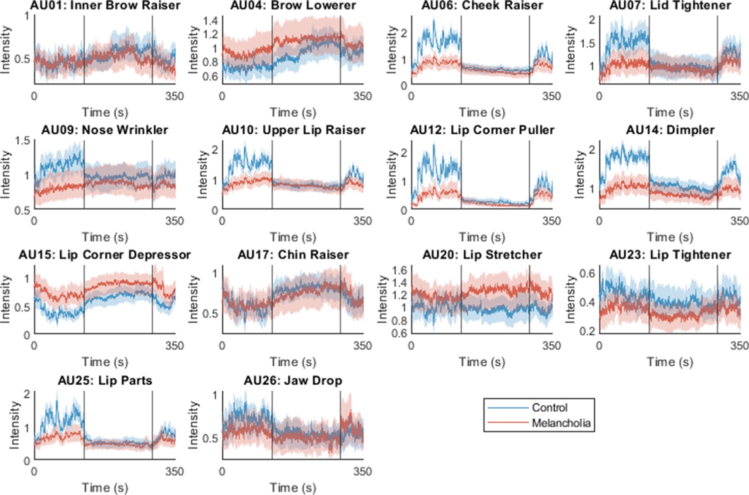
Mean facial action unit activation in controls and melancholia for all action units.
Shaded confidence bands were calculated as the 5th and 95th percentile in a bootstrap sample (n=1000). Participants watched, in sequence, stand-up comedy, a sad video, and a funny video. Vertical lines demarcate transitions between video clips.
Figure 5 with 1 supplement
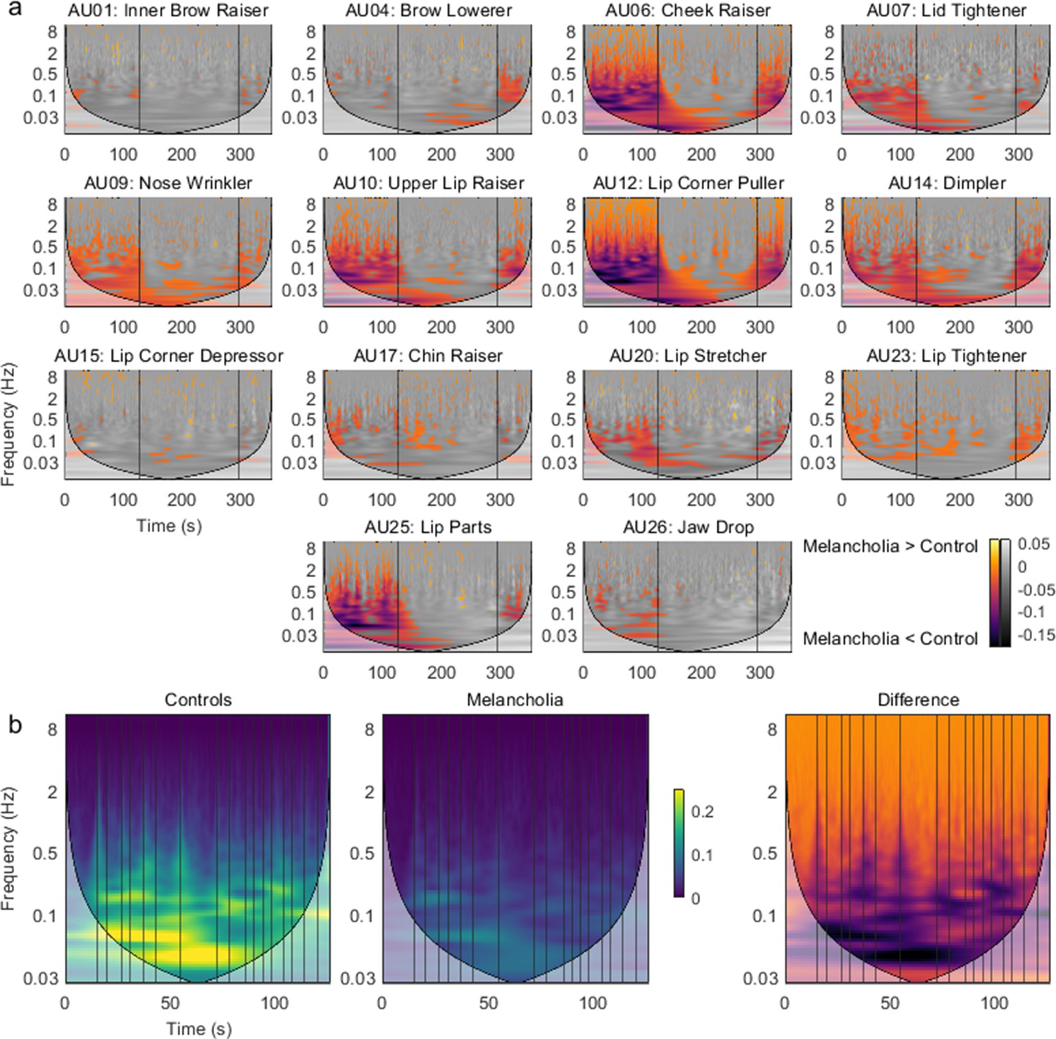
Group differences in time-frequency activity.
(a) Mean time-frequency activity in melancholia benchmarked to the control group. Negative colour values (red-purple) indicate melancholia < controls (p<0.05). Non-significant group differences (p>0.05) are indicated in greyscale. Vertical lines demarcate stimulus videos. (b) Action unit 12 ‘Lip Corner Puller’ during stand-up comedy in controls, participants with melancholia, and difference between groups. Vertical lines indicate joke annotations.
Figure 5—figure supplement 1
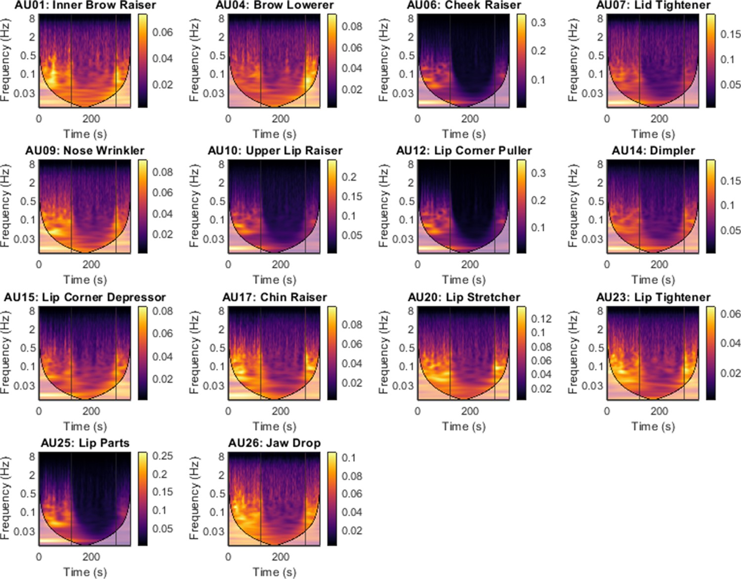
Mean of time-frequency representation across all controls in melancholia dataset.
Participants watched, in sequence, stand-up comedy, a sad video, and a funny video. Shading indicates the cone of influence. Vertical lines demarcate video clips.
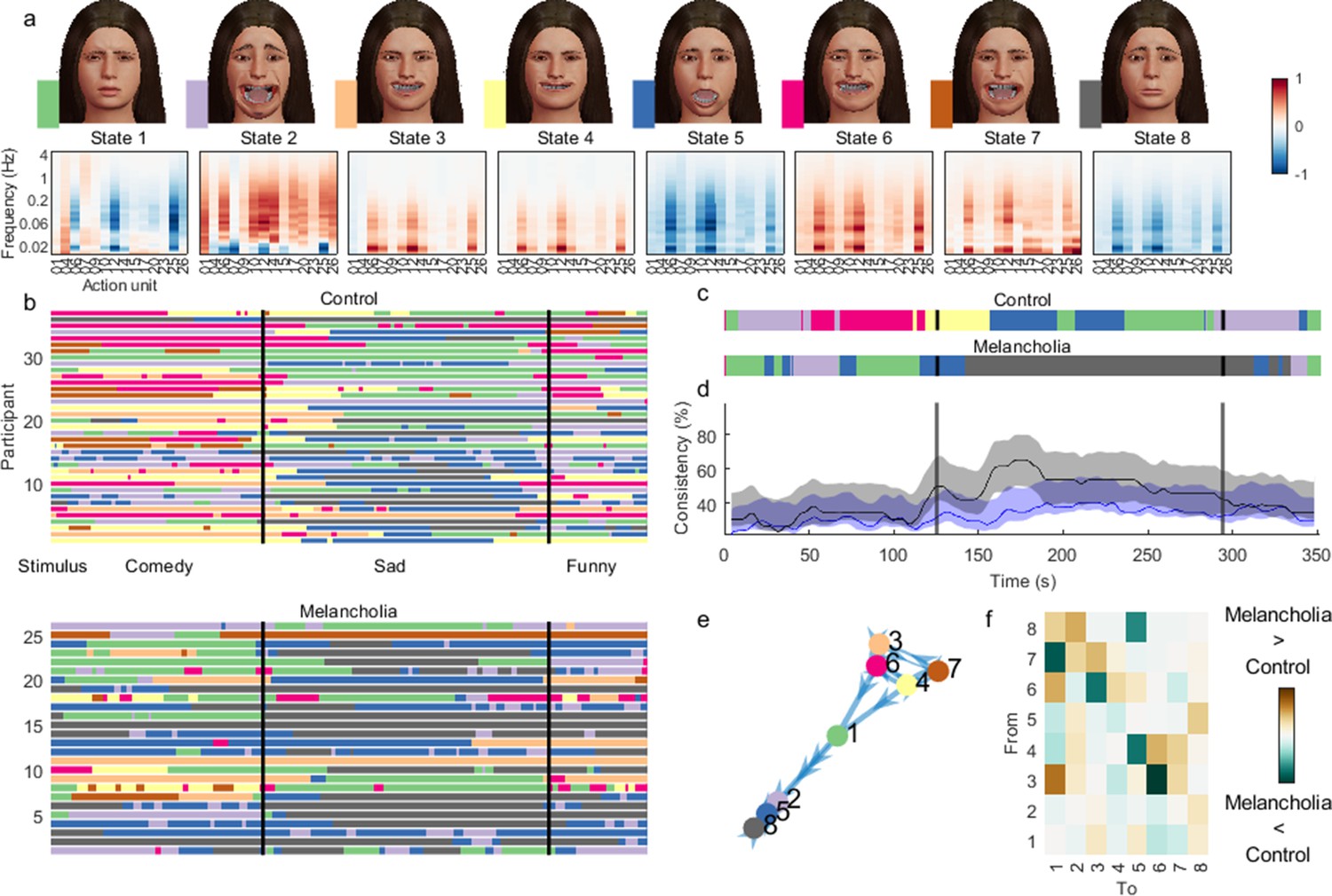
Figure 6 with 2 supplements

Hidden Markov model (HMM) inferred from time-frequency representation of melancholia dataset.
(a) Contribution of action units and their spectral expression to each state. Avatar faces for each state show the relative contribution of each action unit. (b) State sequence for each participant at each time point, for controls (top) and participants with melancholia (bottom). Vertical lines demarcate stimulus clips. (c) Most common state across participants, using a 4 s sliding temporal window. (d) Proportion of participants expressing the most common state for control (blue) and melancholia cohorts (black). Shading indicates 5% and 95% bootstrap confidence bands. (e) Transition probabilities displayed as a weighted graph, with the top 20% of transition probabilities shown. States are positioned according to a force-directed layout where edge length is the inverse of transition probability. (f) Differences in mean transition probabilities between participants with melancholia and controls. Each row/column represents an HMM state. Colours indicate (melancholia–controls) values.
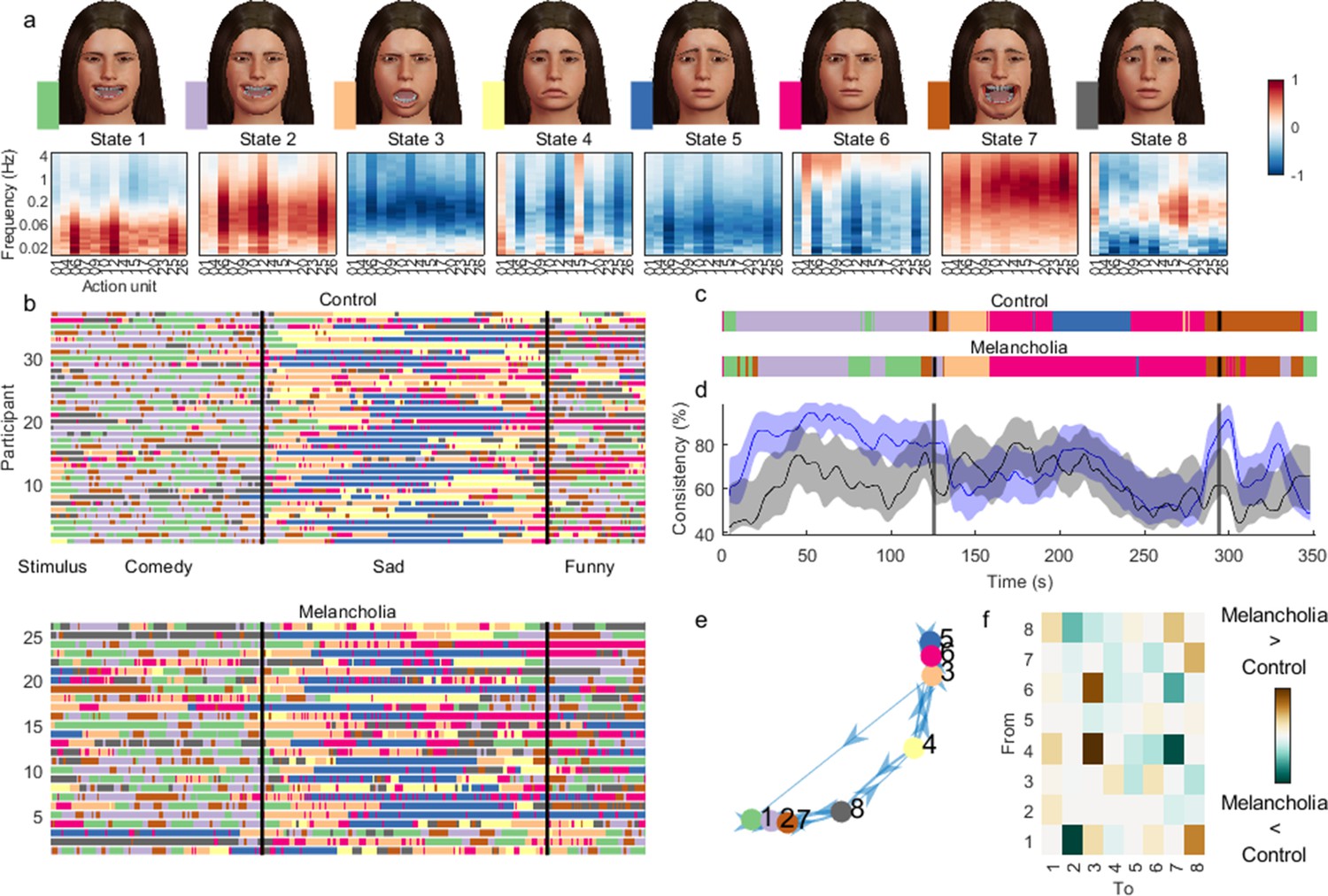
Figure 6—figure supplement 1
Hidden Markov model inferred from time-frequency representation of melancholia dataset, where data are not standardised before model inference.
(a) Mean of the observation model for each state. Avatar faces for each state show the relative contribution of each action unit. (b) Most likely state sequence for each participant at each time point, for controls (top) and participants with melancholia (bottom). Vertical lines demarcate stimulus clips. Without standardisation, state transitions are infrequent and transition probabilities less meaningful. (c) Most common state across participants, using a 4 s sliding temporal window. (d) Proportion of participants expressing the most common state for controls (blue) and participants with melancholia (black). Shading indicates 5% and 95% bootstrap confidence bands. (e) Transition probabilities displayed as a weighted graph. Only the top 20% of transition probabilities are shown. States are positioned according to a force-directed layout where edge length is the inverse of transition probability. (f) Differences in mean transition probabilities between participants with melancholia and controls.
Figure 6—figure supplement 2
Hidden Markov model inferred from time-frequency representation of melancholia dataset, with states defined by a diagonal covariance matrix.
Contents of (a–f) are otherwise identical to Figure 6—figure supplement 1.
Tables
Table 1
Demographics and clinical characteristics.
| Healthy controls | Melancholia | Group comparison,t or χ2, p-value | |
|---|---|---|---|
| Number of participants | 38 | 30 | – |
| Age, mean (SD) | 46.5 (20.0) | 46.2 (15.5) | 0.95 |
| Sex (M:F) | 13:19 | 17:13 | 0.21 |
| Medication, % yes (n) | |||
| Any psychiatric medication | 7% (1) | 85% (23) | – |
| Nil medication | 93% (13) | 15% (4) | – |
| Selective serotonin reuptake inhibitor | 7% (1) | 15% (4) | – |
| Dual-action antidepressant* | 0% (0) | 48% (13) | – |
| Tricyclic or monoamine oxidase inhibitor | 0% (0) | 19% (5) | – |
| Mood stabiliser† | 0% (0) | 11% (3) | – |
| Antipsychotic | 0% (0) | 33% (9) | – |
-
*
For example, serotonin noradrenaline reuptake inhibitor.
-
†
For example, lithium or valproate.
Additional files
-
MDAR checklist
- https://cdn.elifesciences.org/articles/79581/elife-79581-mdarchecklist1-v2.docx
-
Supplementary file 1
Additional data.
- https://cdn.elifesciences.org/articles/79581/elife-79581-supp1-v2.doc
Download links
A two-part list of links to download the article, or parts of the article, in various formats.
Downloads (link to download the article as PDF)
Open citations (links to open the citations from this article in various online reference manager services)
Cite this article (links to download the citations from this article in formats compatible with various reference manager tools)
Quantifying dynamic facial expressions under naturalistic conditions
eLife 11:e79581.
https://doi.org/10.7554/eLife.79581


