Dynamics of cooperative excavation in ant and robot collectives
- School of Engineering and Applied Sciences, Harvard University, United States
- Department of Molecular and Cellular Biology, Harvard University, United States
- Center for Brain Science, Harvard University, United States
- Department of Physics, Harvard University, United States
- Department of Organismic and Evolutionary Biology, Harvard University, United States
Figures
Figure 1
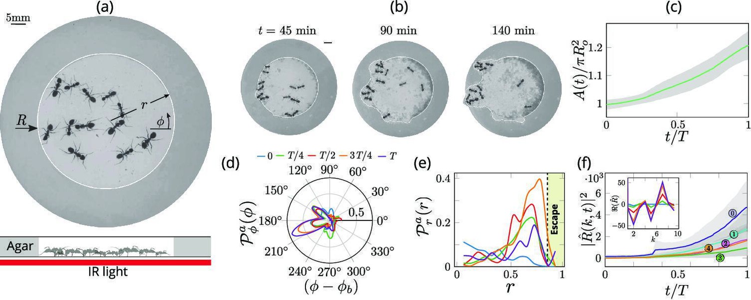
Collective dynamics of ant excavation.
(a) Colony members of the black carpenter ant Camponotus pennsylvanicus are confined to a porous boundary made out of Agarose. The boundary is represented by its radius ( - polar angle, - time). Bottom part shows the side-view schematic of the experimental set-up with the boundary made of agarose and background IR light source used to image the ants in the dark. (b) Temporal progression of excavation experiments as 12 ants cooperatively tunnel through the agarose confinement. The white line is the tracked location of the inner wall which grows in size as the excavation progresses. (c) Confinement area as a function of time (scaled by time to excavate out of the corral ), normalized by initial circular confinement with radius . (d) Evolution of the orientation distribution of the ant density, obtained by averaging along the radial direction. Ants start from an initially isotropic state and localize at an angle along the boundary. here is the excavation time. (e) Dynamics of the radial distribution of ant density as a function of radial distance, obtained by averaging a sector of around the excavation site. We see that the ant density front propagates through the corral. The density is plotted for the same times as in (f) Evolution of the power spectrum of first five Fourier modes capturing the number of tunnels formed during excavation . Inset shows the real part of the Fourier coefficient, at different time instants indicating that many modes are present in the boundary shape.
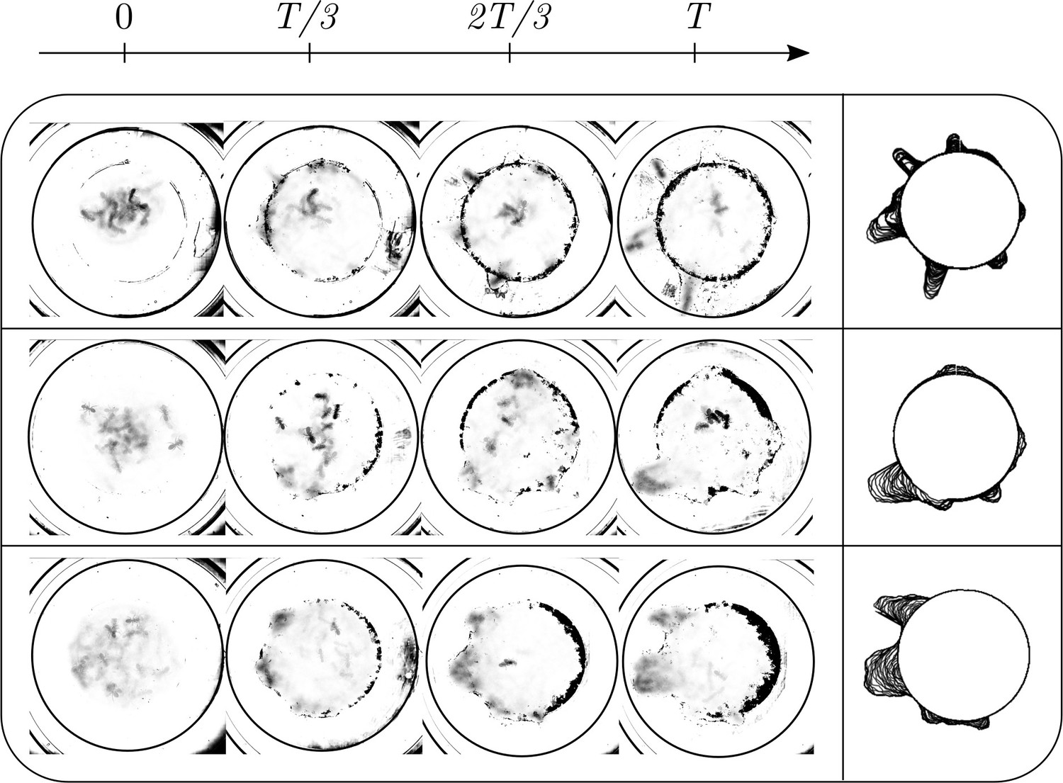
Figure 2
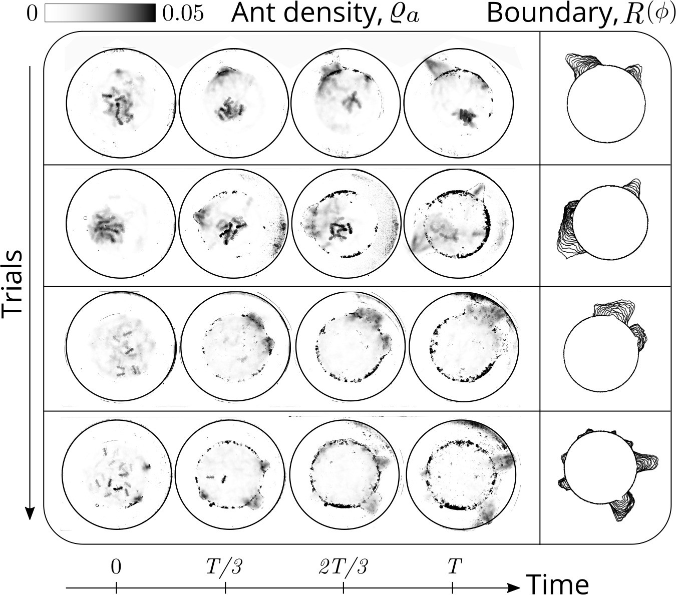
Evolution of the ant density field, (in units of #/mm2) as the tunneling progresses for experiments with 12 major ants.
The density field is obtained by averaging the ant locations over 250 s during the tunneling process. In the second columns is the evolution of the boundary shape, as a function of time where we see multiple excavation sites being explored before one of them succeeds. The darker spots in the image are the debris that the ants deposit as they excavate the boundary.
Figure 3
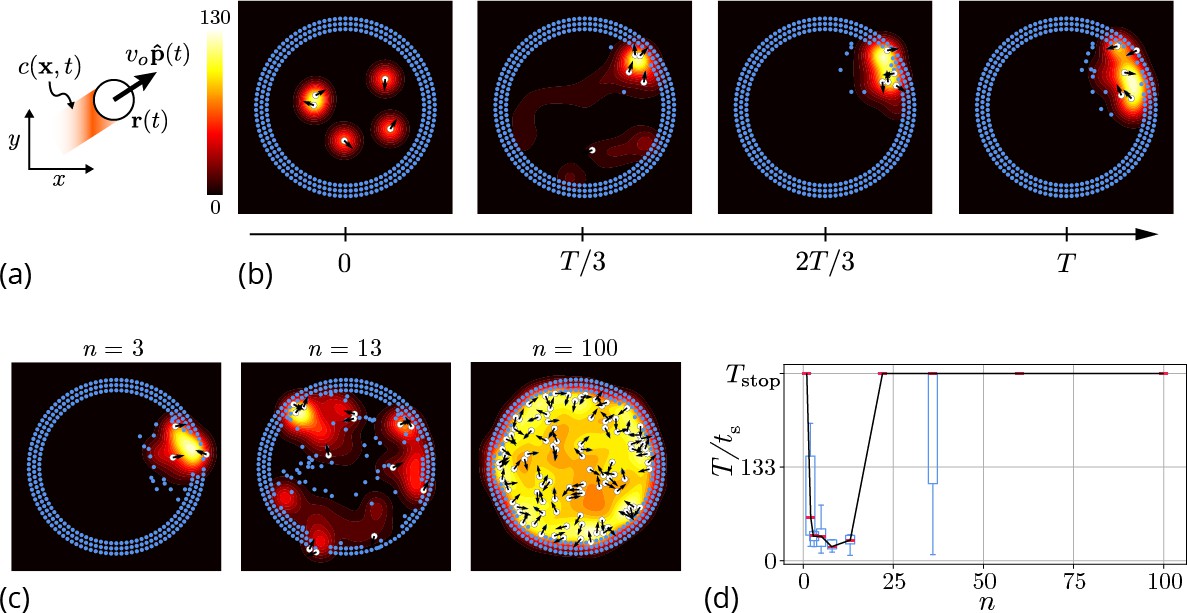
Agent-based simulation.
(a) Schematic of the agents in our simulation captured by their position and orientation moving at speed vo. These agents generate an antennating field at a constant rate which decays at a rate . (b) Progression of cooperative excavation of the corral by 5 agents as they pick elements from the boundary and drop them in the interior (see sec. Appendix 2—table 1 for parameters). Color bar shows the magnitude of antennating field and it varies between 0–130. (c) Snapshot of the dynamics at the end of simulations corresponding to for the number of agents . We see that agents can go from excavating successfully to being trapped in their own communication field. (d) Box plot showing the time taken to excavate out of the corral (non-dimensionalized using - time taken for an agent to travel the entire domain) as a function of the number of agents in the corral when . For very small and very large number of agents the collective does not excavate out as the median and they escape fastest for .
Figure 4
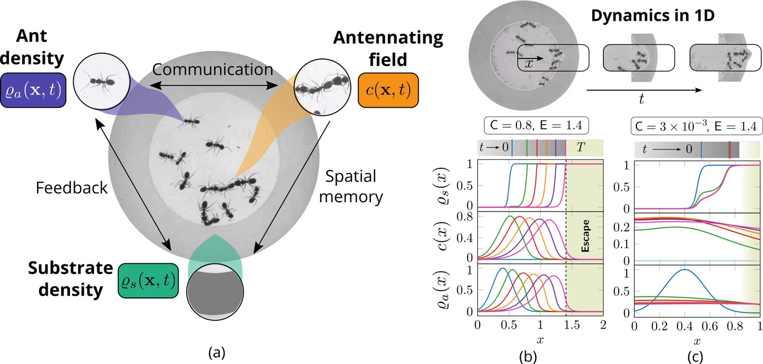
Cooperation via organism-environment-organism interaction.
(a) Schematic of the model showing the interaction between the different spatio-temporal fields required to capture cooperative excavation of ants: ant density, ; concentration of antennating field, capturing inter-ant communication; density of corral, representing the soft corral which the ants excavate. We capture the dynamics of excavation by ants close to the excavation site using the one-dimensional version of Equations 3–5. (b, c) Temporal progression of the corral density, antennating field and the ant density showing successful excavation for high cooperation captured using the non-dimensional number, C (representing non-dimensional strength of cooperation amongst ants) and faster excavation, captured using E. For reduced cooperation ants’ diffusion dominates and only partial tunnels are formed (see Appendix 2 for details). here is the time for excavating out of the corral. The agent density is a gaussian function centered around .
Figure 5
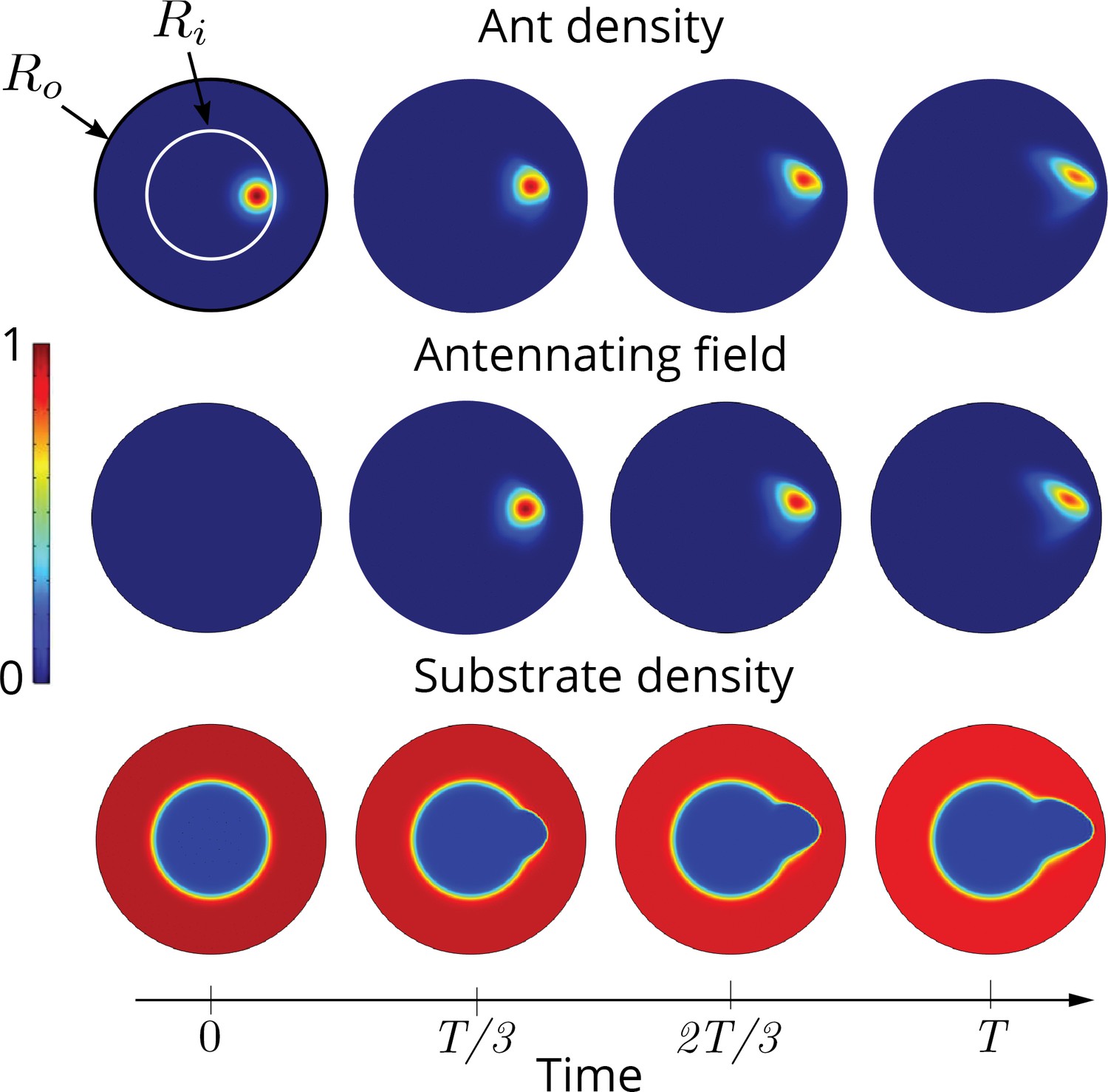
Two dimensional simulations showing the evolution of the ant density , antennating field and the corral density by evolving Equations 3–5, capturing successful tunneling for non-dimensional numbers and time of simulation .
The list of dimensional parameters used in the simulation are indicated in the Appendix 1—figure 1(f). Radius of the outer boundary, is 5 non-dimensional units and the inner boundary is (see Appendix 2 for details). Color bar shows the magnitude of different variables and they vary between 0 and 1.
Figure 6
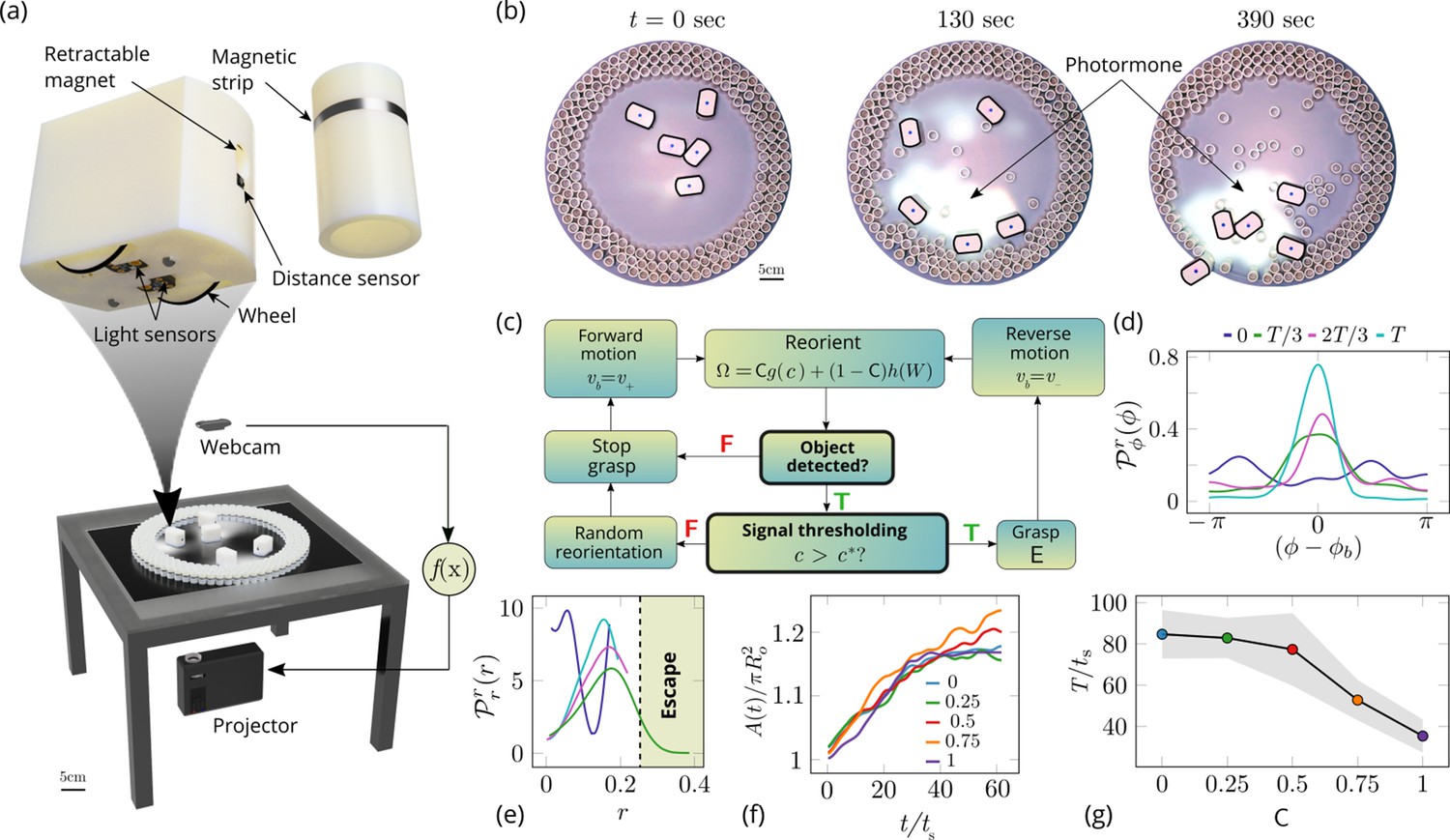
Emergent cooperative excavation dynamics in robotic ants.
(a) Robot Ant (RAnt) set-up. A mobile RAnt is placed in an arena 50 cm in diameter surrounded by three layers of cylindrical boundary elements totalling 200 elements. The outermost layer is prevented from being pushed out of the arena by a circular ring. A scalar concentration field (photormone field) is projected onto a plane whose intensity can be measured by a RAnt. The position of each RAnt is tracked using a webcam. Each RAnt can pick up and drop the discrete boundary elements using a retractable magnet. (b) Series of snapshots at different times of the excavation process for a cooperation parameter C=1. (c) Flowchart of the RAnt programming. A base locomotion speed vb is stored internally and the rate of change of the heading is a function of the cooperation parameter C, the photormone concentration , and a stochastic process (Brownian motion). A photormone threshold determines whether an object is grasped (with probability E) after it is detected by the distance sensor. (d) Orientation distribution of the RAnt density as a function of the azimuthal position is the orientation of the excavated tunnel. The density is plotted for different times. (e) Radial distribution of the RAnt density within a sector of centered around the position of the excavated tunnel as a function of distance from the center of the arena . The density is plotted for the same times as in (d). (f) Confinement area as a function of time, normalized by initial circular confinement with radius for different cooperation parameter C. (g) Normalized excavation time as a function of cooperation parameter C, averaged over 5 experiments per cooperation parameter. Every experiment was run until the first RAnt excavated out or the experiment duration exceeded 15 min.
Figure 7
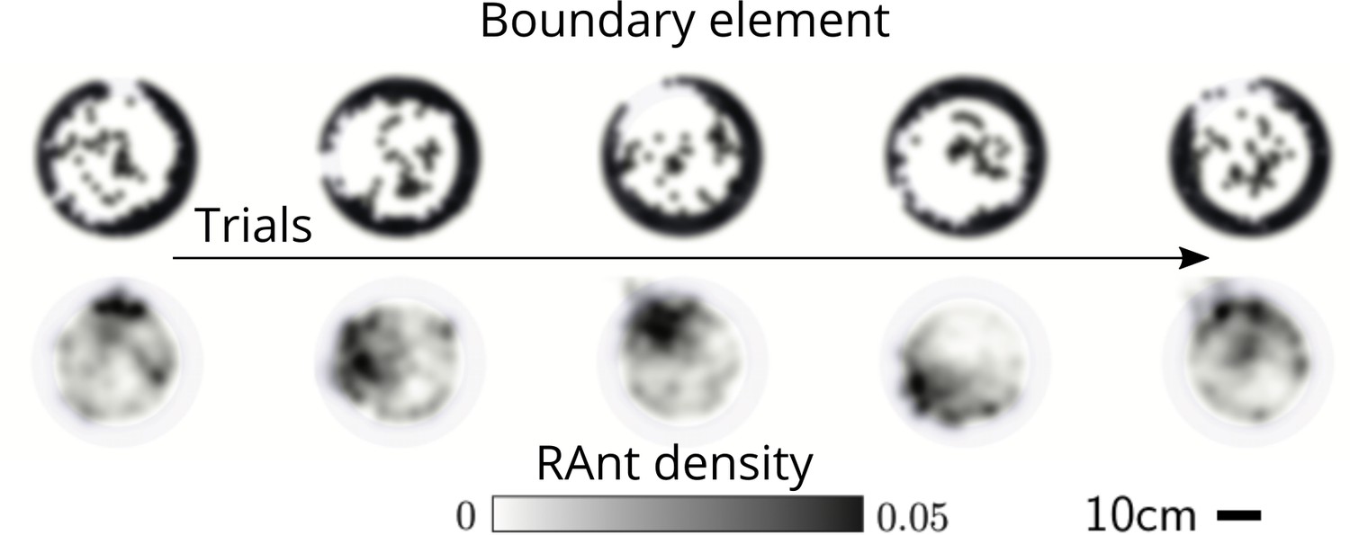
Averaged RAnt dynamics.
Ultimate distribution of boundary elements and averaged RAnt density field (in units of #/cm2) over the full duration of experiments for different trials.
Figure 8
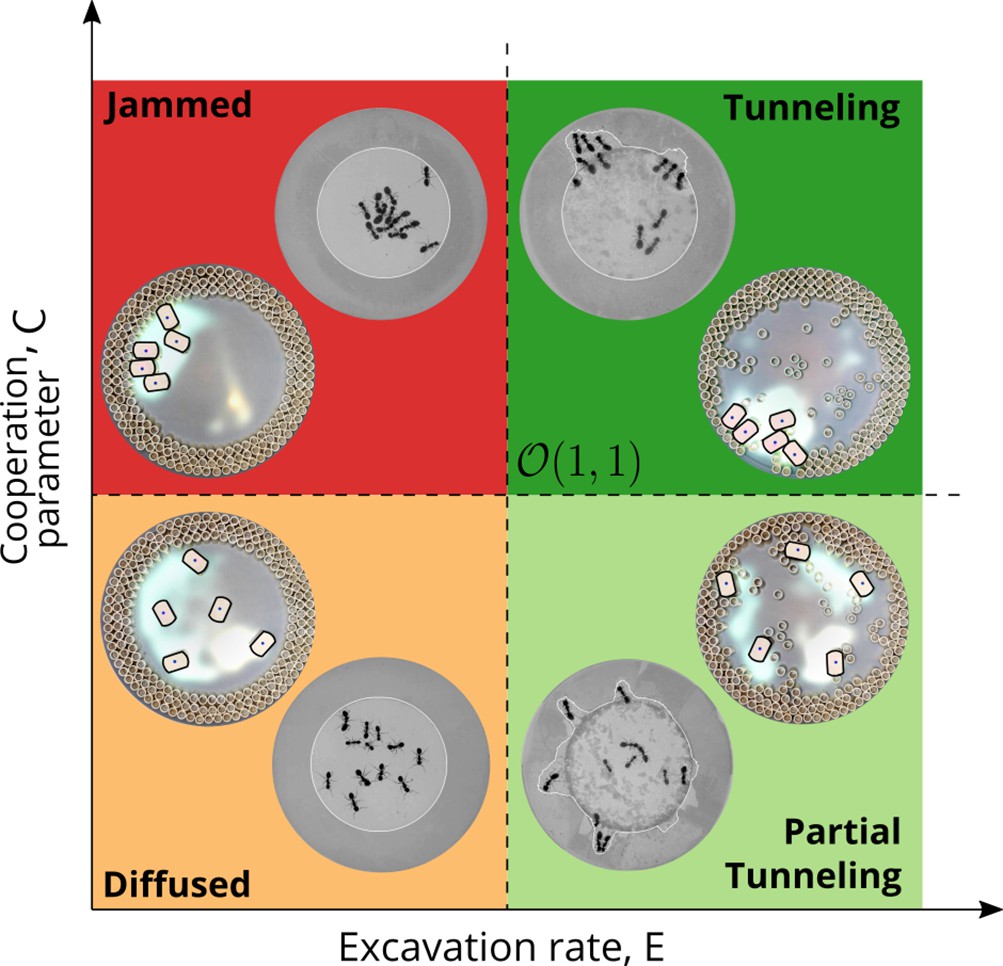
Phases of cooperation Phase-diagram of cooperative task execution with different phases seen in ants and RAnts.
In the robotic experiments we tune the Cooperation parameter C and the Excavation rate E while in the ant experiments we change the caste mixture. In the ant experiments we see the jammed and diffused phases transiently before the ants relax to cooperative excavation.
Appendix 1—figure 1
Dynamics of ant density field, (in units of #/mm2) obtained by averaging the ant location and the boundary shape when 4 ants each of major, media and minor types are confined inside the agar ring for different trials.
Appendix 1—figure 2
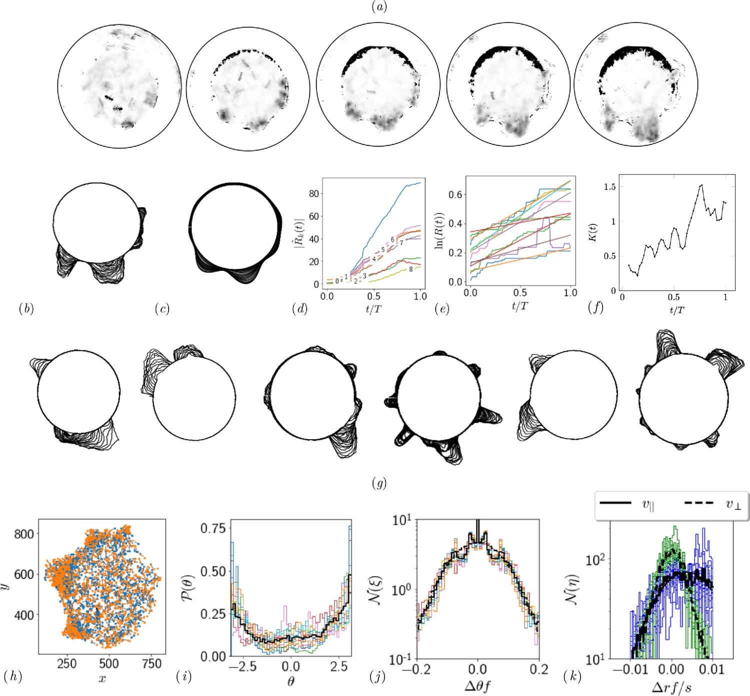
Quantifying competition between different modes of exploration and the transition towards exploitation.
(a, b) Shape of the boundary tunnel during the tunneling process and the approximate representation of the shape using first 9 Fourier modes. (c) Evolution of the magnitude of the first 9 Fourier modes of the boundary: . (d) Evolution of boundary location, at different values and the excavation rate. (g) Collage of boundary evolution showing tunnel formation in six experiments. (e) Location and orientation of the ants obtained from tracking the gaster (orange) and heat (blue) of all the ants. (f) Is the von Mises parameter highlighting strength of focus in ant orientation thorough a fit to the obtained by a curve fit to the distribution. (g) Image showing evolution of the boundary as the excavation process happens for different experimental trials. (h) Location of center of ants with orientation during the excavation process. (i) Average orientation distribution of all the ants showing hints of localization which is evident when plotted over time. (j) Noise statistics of ant velocity along the body axis, and in the normal direction, . Dashed lines again are Gaussian fit to the data. Ants have zero mean velocity normal to its axis. (k) Noise statistics of orientation with peak close to 0 because of resting of the ants which otherwise follows a Gaussian which is the dashed line.
Appendix 2—figure 1
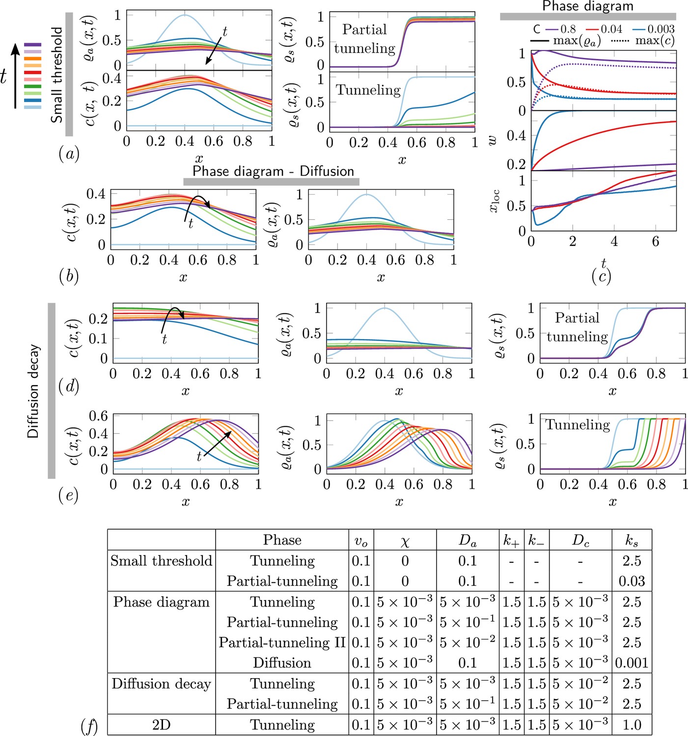
The ant density field, antennating field and corral density for various scenarios of interest in the phase-space.
(a) Partial tunneling and tunneling when the threshold for excavation is small i.e. , we see homogeneous excavation and can get tunneling and partial tunneling; (b) when we are in the diffusive phase where ant density diffusion dominates, and the excavation rate is very small, ; (d, e) partial tunneling and tunneling when the length scale due to antennating field diffusion and decay is of the same order as the initial ant density i.e. ; (c) Evolution of maximum value of for 3 different C and fixed . (f) Table with parameters used in simulations corresponding to different titles shown in gray bar in
Appendix 3—figure 1
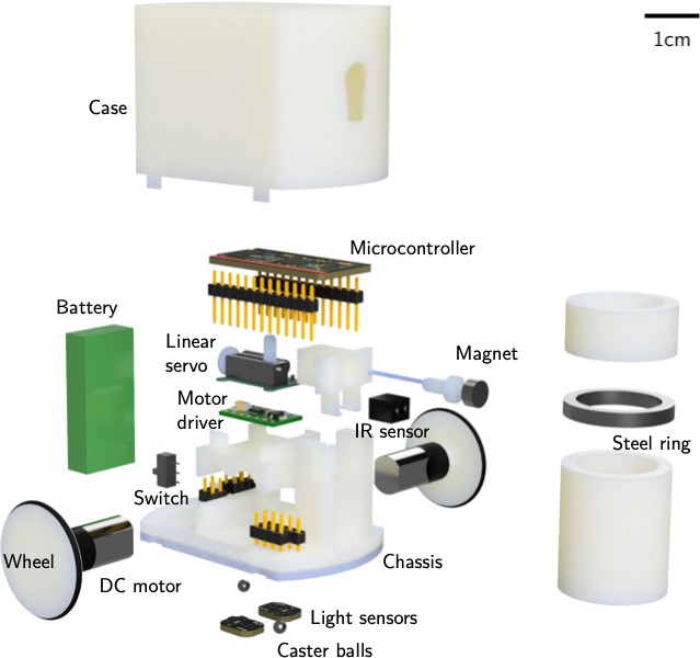
Exploded view of a RAnt and a wall element.
Appendix 3—figure 2
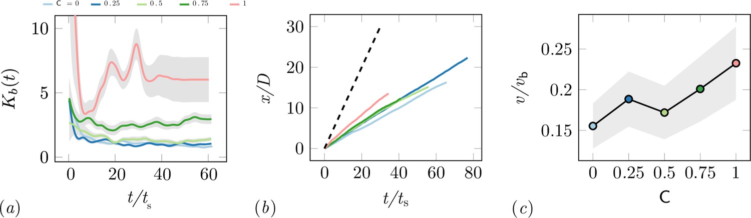
Characterization of the excavation using the von-Mises distribution.
(a) Von Mises concentration parameter, , of the angular position of the excavated boundary elements as a function of time for different cooperation parameters and averaged over 5 experiments per cooperation parameter. (b) Total travelled distance of RAnts for different cooperation parameters. The travelled distance is scaled by the size of the arenda . The dashed line shows the travelled distance of a RAnt moving at base speed vb constantly. (c) RAnts’ averaged speed normalized by for different cooperation parameters C.
Appendix 3—figure 3
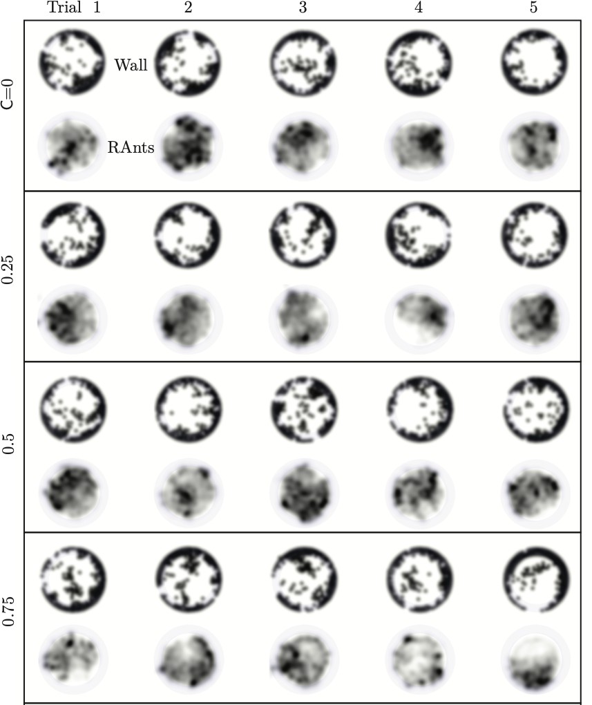
Final wall element distribution and averaged RAnt density field (in units of #/cm2) over the full duration of the run for all 20 experiments.
Appendix 3—figure 4
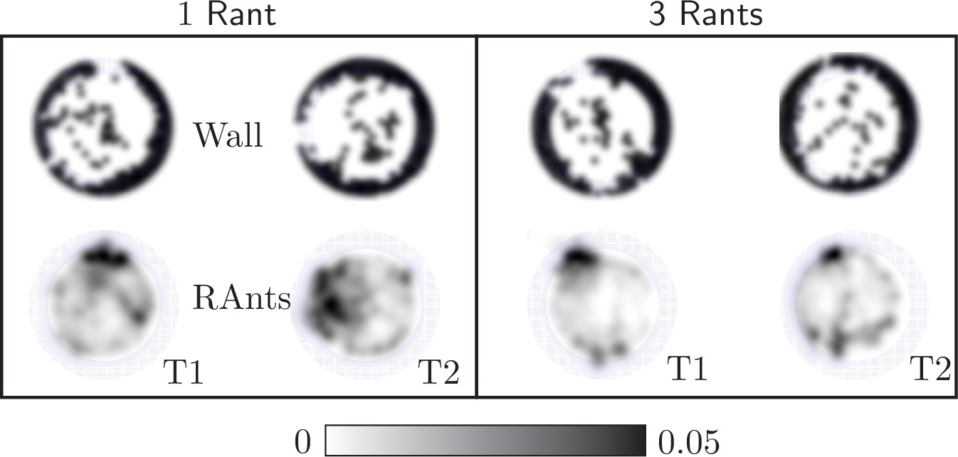
Final wall element distribution and averaged RAnt density field (in units of #/cm2) over the full duration of the run for experiments with one and three RAnts.
The cooperation parameter was set to and the experiments was repeated twice (Trials T1 and T2).
Appendix 3—figure 5

From the RAnt experiments in Figure 8, is the von Mises concentration parameter computed from the location of the boundary and is the angular distribution of the RAnts in the arena averaged over time.
is the time-averaged mean azimuthal location of the RAnts in the arena. RAnts present over longer periods in a particular sector of the arena will cause a peak in . One can infer the phase the RAnts are in by measuring these two quantities.
Videos
Video 1
Ant experiments.
Single ant: We confined 1 ant (major, media and minor individually) and capture their dynamics to see if they are capable of tunneling on their own; Multiple castes assemblage: We confined 12 ants, 4 for each of major, minor and media castes, and capture the dynamics of excavation as they tunnel through the boundary; Major ant collective excavation: We confined 12 major ants and capture the dynamics of excavation as they tunnel through the boundary.2.
Video 2
Dynamics of excavation from agent-based simulation for different number of agents () in the corral for parameters in tab Appendix 2—table 1 We see successful escape as well as trapped dynamics as highlighted in Figures 3 and 4.
Video 3
Successful tunneling in RAnts.
Dynamics of excavation by RAnts as they cooperatively tunnel through the corral for and without cooperation, ; Jammed phase: When the pick-and-place in RAnts is deactivated (corresponding to ), they get jammed for ; Diffused phase: When the pick-and-place in RAnts is deactivated and the RAnts do not follow the antennating field (corresponding to ), they diffuse around.3.
Video 4
Summary video showing the results from ant experiments, theoretical model and robot experiments.
Tables
Table 1
List of relevant variables and basic behaviors, for ant experiments, theoretical models and robotic implementation.
| Ants | Theoretical model | Robots |
|---|---|---|
| Discrete ants | Ant density, | Discrete robots |
| Antennae communication | Communication field, | Photormone field |
| Agarose corral | Substrate density, | Boundary elements |
| Motility | Self-propulsive advection, | Mobile agents |
| Exploratory behavior | Density diffusion, | Random walk |
| Tactile feedback | Antennating field taxis, | Phototaxis |
| Biting behavior | Excavation rate, ks | Collection and deposition |
| Neural control | Dynamics of ant density | Behavioral rules |
Appendix 2—table 1
Parameters of agent-based simulation.
| Parameter | Description | Value |
|---|---|---|
| nr | Number of agents | 1–100 |
| no | Number of substrate elements | 300 |
| nl | Number of corral layers | 3 |
| Maximum simulation time | 66 | |
| Communication field production rate | 97.5 | |
| Communication field decay rate | 0.75 | |
| Communication field diffusivity | ||
| Excavation threshold | ||
| Detachment threshold | 0.11 | |
| Agent field production width (variance) | ||
| ld | Agent obstacle detection range | 0.03 |
| Pause after obstacle detection | 0.07 | |
| Pause after substrate attachment | 0.27 | |
| Rotational gain | 0.135 |
Appendix 2—table 2
Time-scales and length-scales associated with different processes in the model in Equation 12- Equation 14.
| Time-scale | Process |
|---|---|
| Ant collective migration | |
| Taxis due to antennating field gradient | |
| Antennating field production | |
| Antennation field diffusion | |
| Antennating field decay | |
| Corral excavation | |
| Length-scale | Process |
| Corral width | |
| la | Initial width of ant density |
| Ant density advection-diffusion | |
| Antennating field diffusion-decay | |
| Ant diffusion |
Appendix 2—table 3
Different phases in different limits of phase-space of parameters in the model.
| Phase | |||||
|---|---|---|---|---|---|
| Tunneling | |||||
| Tunneling | |||||
| Partial-Tunneling | |||||
| Partial-Tunneling | |||||
| - | Jammed | ||||
| - | Jammed | ||||
| - | - | - | Diffused |
Additional files
Download links
A two-part list of links to download the article, or parts of the article, in various formats.
Downloads (link to download the article as PDF)
Open citations (links to open the citations from this article in various online reference manager services)
Cite this article (links to download the citations from this article in formats compatible with various reference manager tools)
Dynamics of cooperative excavation in ant and robot collectives
eLife 11:e79638.
https://doi.org/10.7554/eLife.79638


