Pallidal neuromodulation of the explore/exploit trade-off in decision-making
- Charité – Universitätsmedizin Berlin, corporate member of Freie Universität Berlin and Humboldt-Universität zu Berlin, Movement Disorder and Neuromodulation Unit, Department of Neurology, Charité Campus Mitte, Germany
- Berlin Institute of Health at Charité – Universitätsmedizin Berlin, Core Facility Genomics, Germany
- Division of Imaging Science and Technology, Medical School, University of Dundee, United Kingdom
- Berlin School of Mind and Brain, Charité - University Medicine Berlin, Germany
- NeuroCure, Charité - University Medicine Berlin, Germany
- DZNE, German Centre for Degenerative Diseases, Germany
- Department of Neurology, Ninewells Hospital & Medical School, United Kingdom
Figures
Figure 1 with 1 supplement

General overview of the study design and task.
(A) Localisation of DBS electrodes was done with Lead-DBS (https://www.lead-dbs.org/) as previously described (; Horn et al., 2019). The left panel depicts electrode localisation within the GPI projected to a 7T brain backdrop (Edlow et al., 2019). On the right panel, active contacts location is shown in red – only two patients (# 6 and #9) show active contacts within the GPe (blue). (B) Each of the two reversal learning task blocks. The blocks differed only in the pair of fractals used as stimulus options. Each reversal learning task block consisted of three 40 trial sessions. Reversal of the probability of receiving a reward occurred half-way through session two. The task was performed once in the OFF- DBS state and once in the ON-DBS state in a counterbalanced manner with a 20 minute break (‘B’) in between blocks 1 and 2. During this, DBS stimulator was either switched ON or OFF. (C) Example of a single trial in the reversal learning task. On each trial, subjects chose either left or right fractal options, which were also counterbalanced, using their left or right hand to press the corresponding keyboard button. The selected cue was then shown surrounded by a red circle (in this example Task Block 1 the left-hand cue is chosen). Subjects were then presented with the outcome of their choice on the next screen, which could be either a reward (‘You Win’) or zero (‘Nothing’). Outcome probabilities of receiving a reward on choosing either fractal were 80%:20%.
Figure 1—figure supplement 1
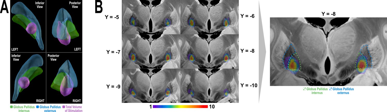
Spatial distribution of stimulation volume on a group level.
(A) 3D rendering of total volume of stimulation (purple) summed for n=14 patients illustrated in relation to the GPi (green) and GPe (blue) nuclei. (B) 2D coronal slices (Edlow et al., 2019) of n-map representing voxel-wise heat-map of how many stimulation volumes are overlapping in each voxel of the total stimulation volume. The slices are selected to cover the extent of the total stimulation volume from most anterior to most posterior aspect. Of note, the majority of the stimulation volumes were located in the posteroventral part of the GPi as indicated by the red-yellow colour gradient of the heat-map. Voxels overlapped with GPe were covered by ~1–2 stimulation volumes (purple-blue colour) and mainly encroaching on its medial margin (right panel of B). Weighted-sum of overlap between the heat-map and the GPI is 1556.5, while that with the GPe is 376.5. The weighted-sum GPi/GPe ratio of overlap is 4.13, which means that GPi is being stimulated ~4 times more frequently than GPe in our cohort. The maximal overlap value in the heat-map is 10 which is less than patients’ number (n=14). This is because of the fact that the heat-map distribution is governed by spatial heterogeneity of the stimulation volumes and their geometrical configuration.
Figure 2
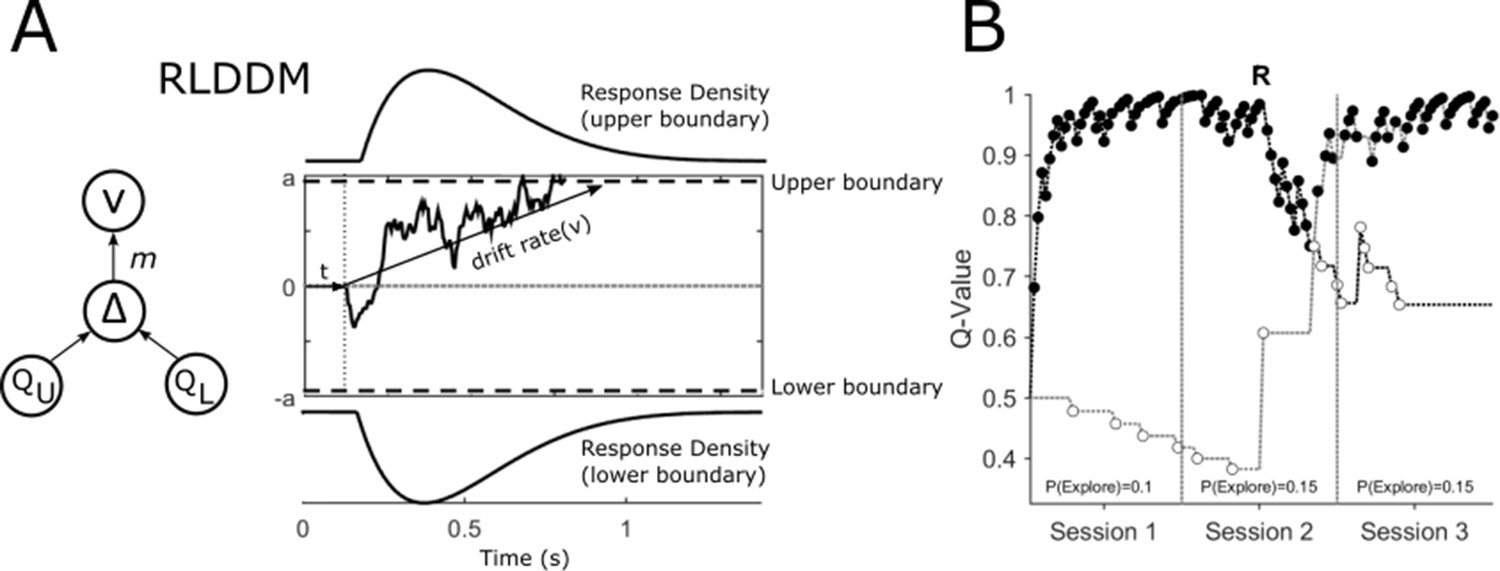
Reinforcement Learning Drift Diffusion Model (RLDDM).
(A) The accumulation of evidence begins at a starting point at 0. The non-decision time is represented by t. Evidence accumulation is represented by a sample path with added Gaussian noise and is gathered until a decision boundary (a and -a) is reached and a response is initiated. The drift rate v determines the rate at which this evidence is accumulated. The extent to which the difference in the expected value of the options of the upper (QU) and lower response boundaries (QL) modifies the drift rate is determined by the drift rate scaling parameter, m. (B) An example of an individual patient’s choices (OFF-DBS, Task Block 1) across the three sessions of the task with the expected value of choices represented by the upper QU and lower QL decision boundaries in black and grey respectively. Closed circles represent ‘exploitative’ choices where the choice with the highest expected value was chosen. Open circles are ‘exploratory’, representing the choice of the lower value of the two options. The change in value of the two choices halfway through session 2 of the task reflects the reversal, ‘R’, in outcome probabilities. The probability of exploring P(Explore) is the total number of choices made for the option with the lower expected value divided by the number of choices made in the session.
Figure 3 with 2 supplements
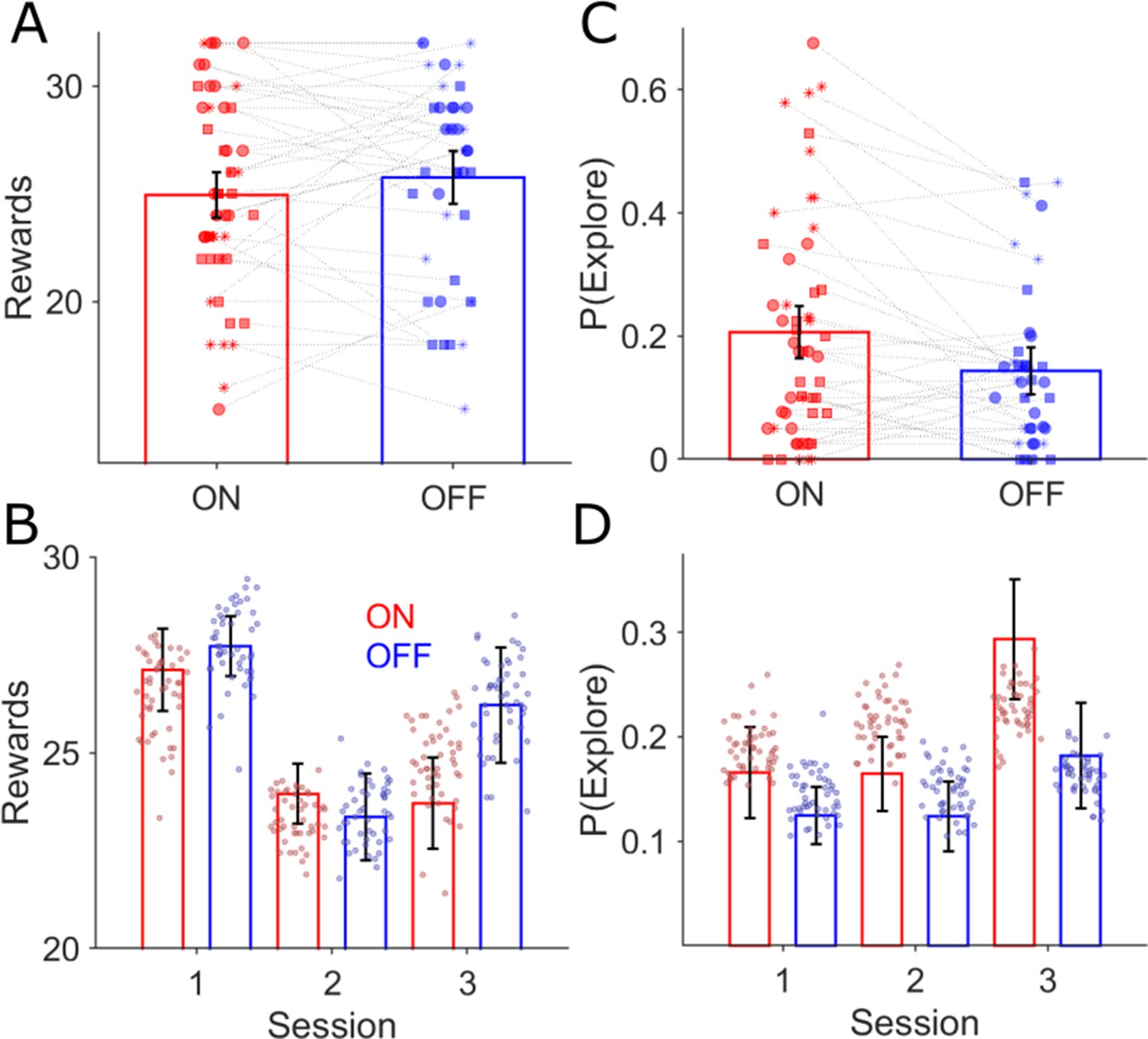
Behavioural effects of GPI DBS on task performance.
There was no difference in the mean rewards (ANOVA, p>0.05) won across the three task sessions for the ON (red bars, n = 18) and OFF-DBS (blue, n=14) conditions (A) and (B) mean ± s.e.m. Each symbol represents a subject’s number of rewards won for that session, with sessions one, two and three represented by the circle, square and asterix symbols. During ON-DBS testing the probability of exploring the lower value choice was significantly greater (ANOVA, p<0.05) (C). Behavioural performance is plotted in (B) (number of rewards) and (D) (probability of exploring the lower value choice) for both DBS conditions with the superimposed scatter plots of the 50 simulated experiments generated using the RLDDM fitted to the ON and OFF experimental choices.
Figure 3—figure supplement 1
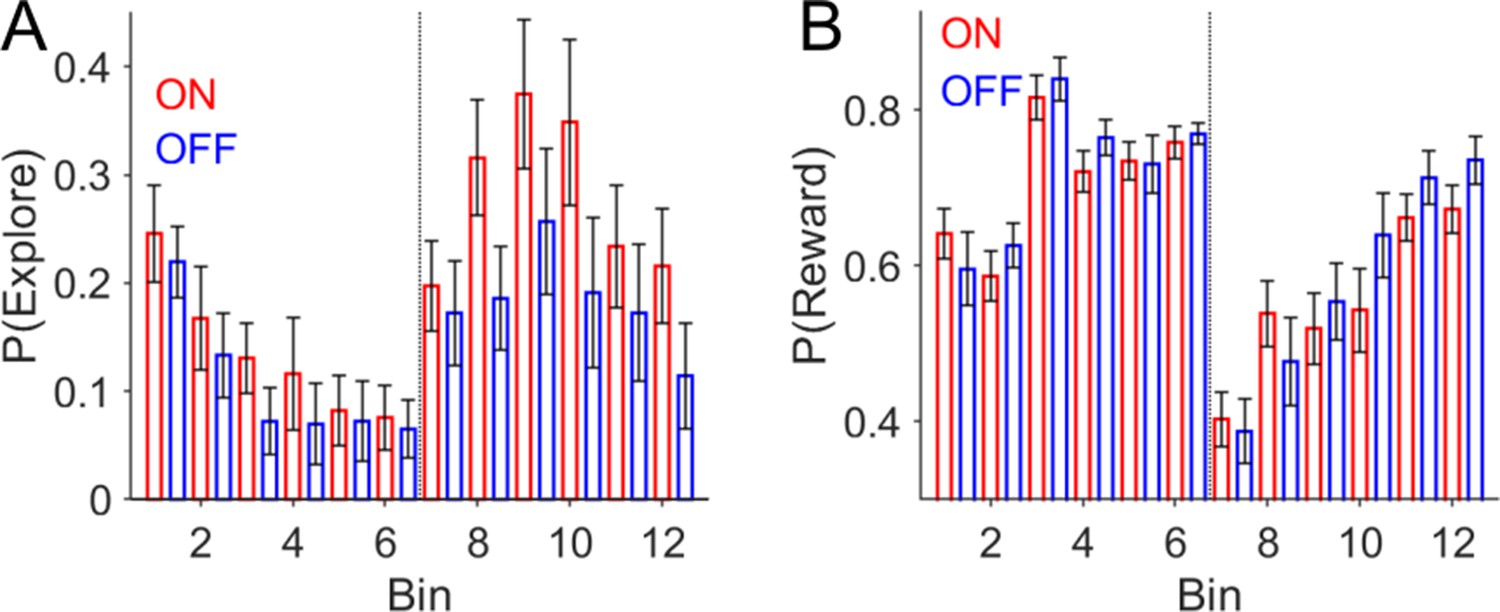
Behavioural effects of GPI DBS on task performance peri- contingency reversal.
(A) Probability of making an exploratory choice P(Explore), plotted as a function of time across twelve 10-trial bins. P(Explore) values are expressed as mean ± s.e.m. with choices ON-DBS in red and OFF-DBS in blue. The vertical dotted line represents the point of contingency reversal in the task (midway through the second experimental session). (B) The probability of a receiving a reward ‘P(reward)’ which is the sum of the number of rewards in bin divided by the number of choices.
Figure 3—figure supplement 2
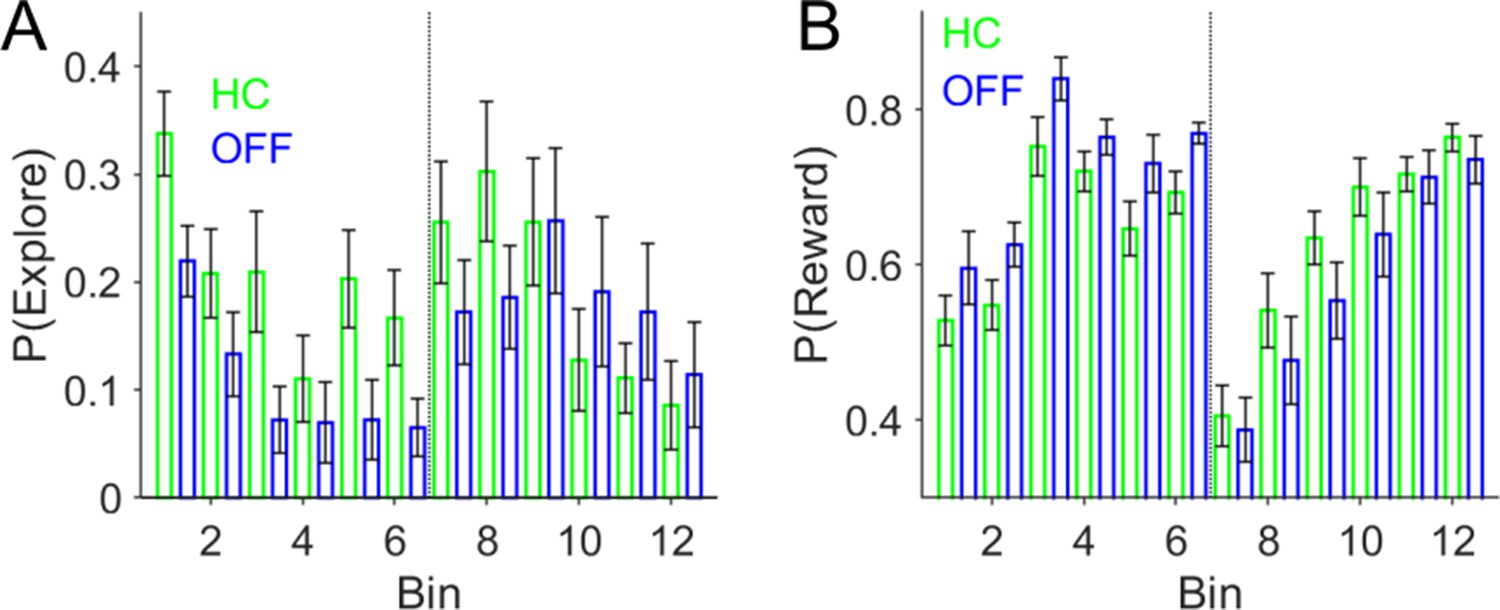
Behavioural performance in Healthy Controls (HC) compared to patients in the DBS-OFF condition.
(A) Probability of making an exploratory choice P(Explore), plotted as a function of time across twelve 10-trial bins. P(Explore) values are expressed as mean ± s.e.m. with HC choices in green and OFF-DBS in blue. The vertical dotted line represents the point of contingency reversal in the task (midway through the second experimental session). (B) The probability of a receiving a reward ‘P(reward)’ which is the sum of the number of rewards in bin divided by the number of choices.
Figure 4 with 1 supplement
Functional connectivity of DBS-Induced exploration.
The whole-brain voxel-wise R-Map demonstrates the optimal functional connectivity profile for DBS-induced enhancement of exploration (B). In this analysis, the maximal increase in DBS induced exploration (ON-OFF DBS) in one of the three experimental sessions was used as the regessor. Warm colours show voxels where functional connectivity to the DBS stimulation volumes was associated with greater exploration. Cool colours indicate voxels where functional connectivity to the DBS stimulation volumes was associated with lesser exploration. The more the individual functional connectivity profile matched the ‘optimal’ R-Map, the greater was the DBS-induced exploration (A) (R2=0.28, p=0.04). In (C) we plot the R value distribution derived from 1000 repermuted correlations between the enhancing effect DBS and the R-map. The probablity of seeing the same correlation by chance was p<0.01 (represented by the red dashed vertical line).
Figure 4—figure supplement 1

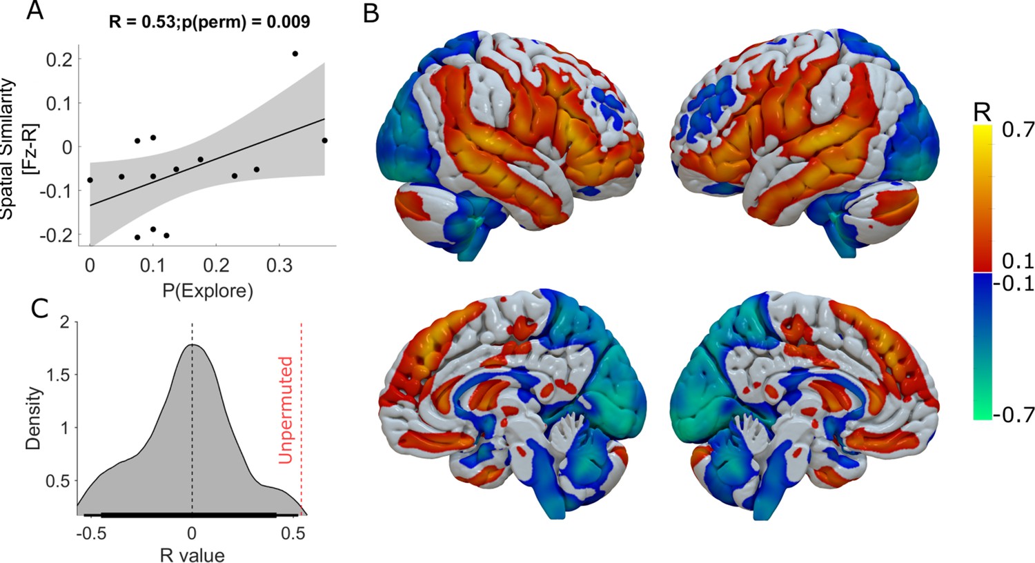
Functional connectivity of DBS-induced exploration.
The whole-brain voxel-wise R-Map demonstrates the ‘optimal' functional connectivity profile for DBS-induced enhancement of exploration. (A) In this analysis, we used the average difference in P(Explore) across the three experimental sessions in the task (ON-DBS minus OFF-DBS). (B) shows the ‘optimal’ R-Map that was associated with the highest DBS-induced exploration when assessed across the whole task. In (C) we plot the R value distribution derived from 1000 repermuted correlations between the enhancing DBS effect and the R-map. The probability of seeing the same correlation by chance was p<0.01.
Figure 5
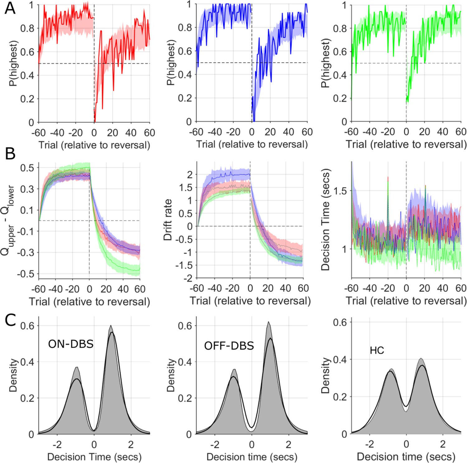
Observed and simulated RLDDM data.
(A) The probability of choosing the highest value stimulus in the ON-DBS state is represented by the solid red line. Overlaid shaded area represents 95% confidence limits of simulated choices of the RLDDM (averaged across 50 simulated experiments). The same analysis for the OFF-DBS state is plotted in blue in the middle panel and for HC in green. This supported the interpretation of the model being a good fit to the experimental data due to the strong overlap between the synthetic data choices and those observed for both DBS conditions and in both HC and patient groups. (B) The difference in the expected value (Q) of the two choices in the RLDDM (mean ± 95% confidence limits) are represented by the solid blue (OFF-DBS), red (ON-DBS) and green (HC) lines with the shaded overlay showing the confidence limits estimated from the synthetic (simulated) data. The middle panel in (B) illustrates the trial-to-trial variation in the mean drift rate, v, across the simulations in all conditions and groups. This demonstrates a reduction in the ON-DBS drift rate consistent with the group level effect of DBS on reducing the drift rate scaling parameter, m, (see Figure 6—figure supplement 1 and Supplementary file 2) and the lower drift rate in the HC group. The mean experimental trial-to-trial variation in DT in each DBS condition and the HC group are plotted as a solid line with the simulated model DT’s overlaid. The model captures both the within task cost of the contingency reversal on DT and the faster DT in the HC group through the task. In (C), thicker black lines display the observed decision time distribution across all patients and sessions in the ON-DBS (red) and OFF-DBS (blue) conditions and HC groups, with the simulated DT from the RLDDM represented by the grey shaded regions. The decision time (DT) for choices which have an initially lower value are shown as negative. The reliability of the RLDDM in capturing the decision mechanisms in the task are supported by the overlap in observed and simulated DT distributions.
Figure 6 with 2 supplements
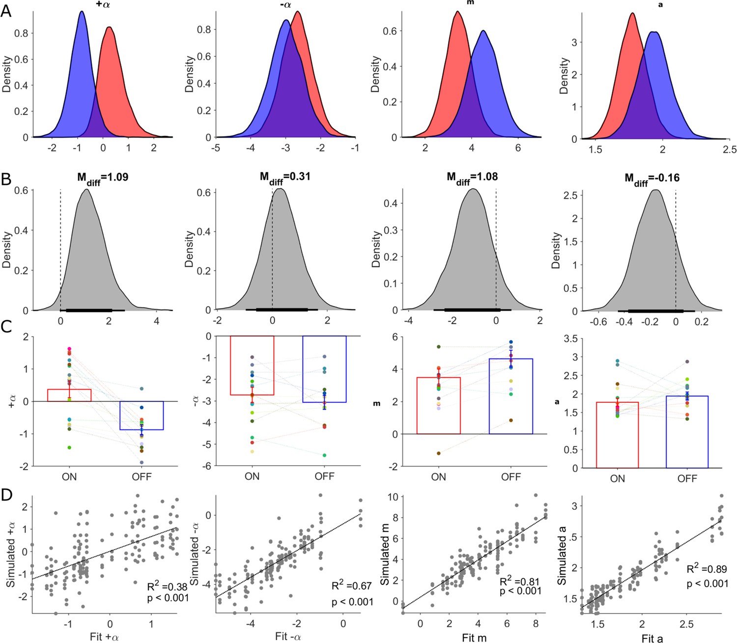
Posterior distributions of RLDDM parameters and parameter recovery.
Columns in this figure display results for each of the estimated parameters in the RLDDM from left to right, including positive learning rate (), negative learning rate (), drift rate scaling parameter (m), boundary separation parameter (a). Rows, from top to bottom, correspond to (A) posterior distributions ON-DBS (red), OFF-DBS (blue). (B) Posterior distributions of differences ON-DBS versus OFF-DBS. Thick and thin horizontal bars below the distributions represent the 85% and 95% highest density intervals, respectively. (C) Mean ± S.E.M. parameter estimate ON-DBS (red) and OFF-DBS (blue). Each individual‘s parameter estimate represented by a different colour in the scatter plot for each parameter. (D) Results of parameter recovery analysis, plotting the estimated parameter values for the observed data against the parameter values re-estimated from simulated data. Significant (p<0.001) linear correlations were observed for all four parameters supporting successful recovery and validation of applying the RLDDM model of decision-making.
Figure 6—figure supplement 1
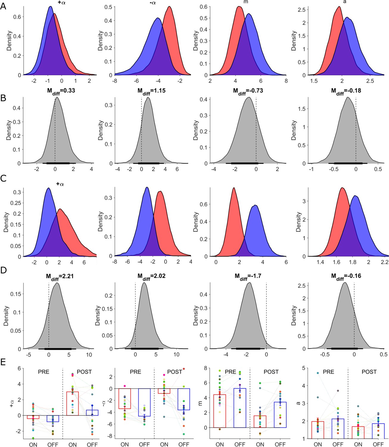
Posterior distributions of RLDDM parameters and parameter recovery – separately fitted to pre- and post- reversal trials.
Columns in this figure display results for each of the estimated parameters in the RLDDM model from left to right including, positive learning rate (), negative learning rate (), drift rate scaling parameter (m), boundary separation parameter (a). Parameter estimates for pre-reversal trials in rows (A) and (B) with posterior distributions ON-DBS (red), OFF-DBS (blue). (B) Posterior distributions of differences ON-DBS versus OFF-DBS. Thick and thin horizontal bars below the distributions represent the 85% and 95% highest density intervals, respectively. Parameter posterior distribution estimates from fitting post-reversal trials in rows (C) and posterior distributions of differences in (D).In row (E) individual subjects parameter estimate after fitting both pre- and post reversal trials, ON (red) and OFF-DBS (blue). The group mean ± S.E.M are plotted. Each individual‘s parameter estimate represented by a different colour in the scatter plot for each parameter.
Figure 6—figure supplement 2
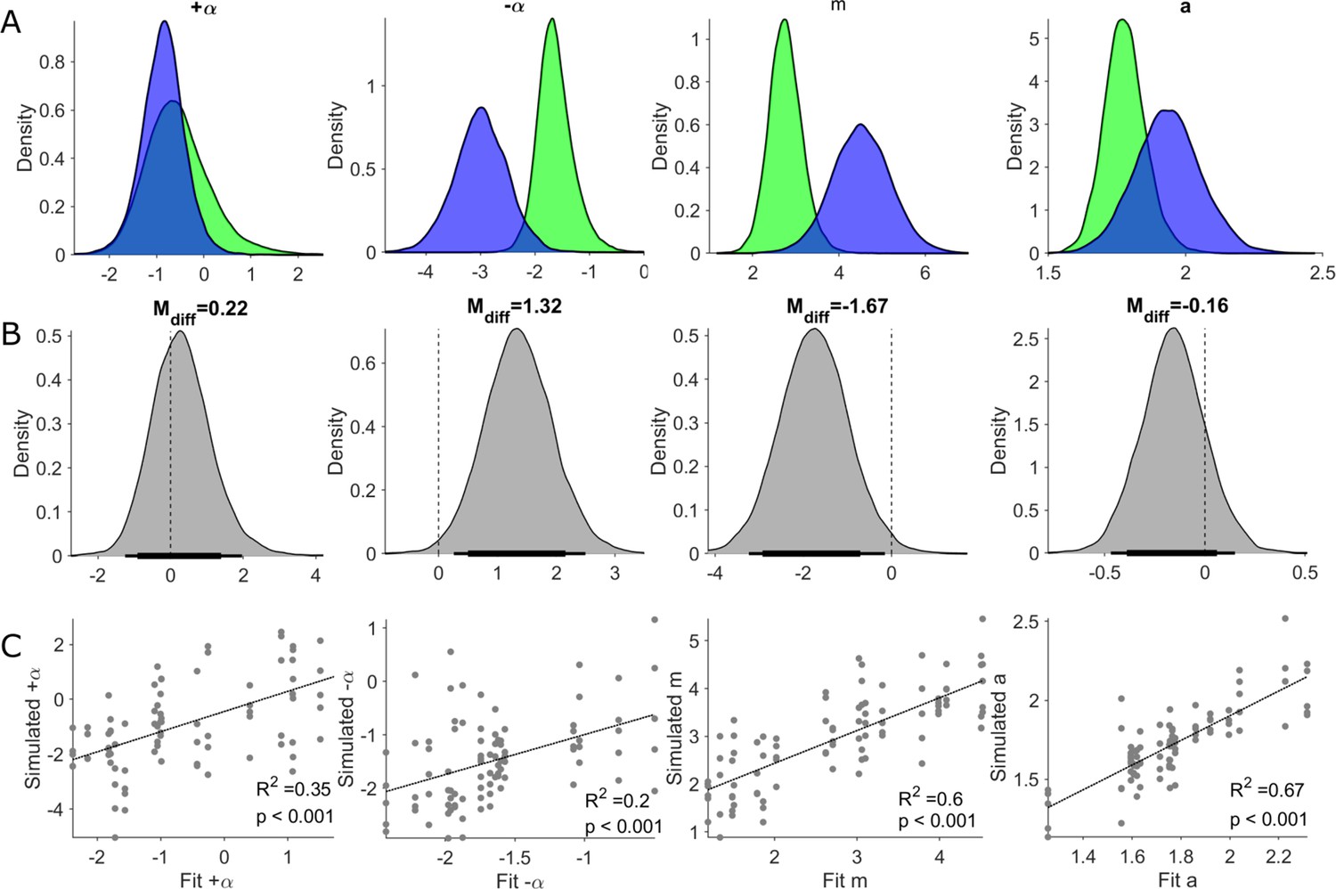
Posterior distributions of RLDDM parameters from Healthy Controls (HC) and parameter recovery.
Columns in this figure display results for each of the estimated parameters in the RLDDM model from left to right, including positive learning rate (), negative learning rate (), drift rate scaling parameter (m), boundary separation parameter (a). Parameter estimates in row (A) and with posterior distributions for HC (green) and OFF-DBS (blue). (B) Posterior distributions of difference between HC minus OFF-DBS. Thick and thin horizontal bars below the distributions represent the 85% and 95% highest density intervals, respectively. (C) Results of parameter recovery analysis, plotting the estimated parameter values for the observed data against the parameter values re-estimated from simulated data. Significant (Pearson's correlation, p<0.001) linear correlations were observed for all four parameters supporting successful recovery of and validation of applying the RLDDM model of decision-making.
Author response image 1
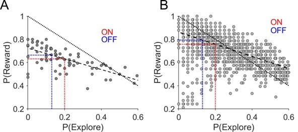
Relationship between task performance P(Reward) and probability of exploratory choices in a session.
(A) Probability of making an exploratory choice in a session plotted against the probability of obtaining a rewarding outcome – P (Reward) – experimental data. (B) Simulated data. Each data point is derived from simulated data choices of the RLDDM performing the reward-reversal learning task (n=50). The dashed line represents the linear fit of this relationship between P(explore) and P(Reward). The dotted line represents a perfect negative linear relationship with slope of -1. The average experimental change in P(Explore) ON-DBS and OFF-DBS is superimposed in red and blue dotted vertical lines with the corresponding change in P(Reward) predicted from this linear fit by the horizontal equivalent line.
Tables
Table 1
Summary of posterior distributions (RLDDM model fit to whole task).
| Parameter | ON-DBS | OFF-DBS | Contrast | |||||||
|---|---|---|---|---|---|---|---|---|---|---|
| mean | HDI | mean | HDI | mean | HDI | |||||
| Boundary separation | 1.78 | 1.56 | 1.98 | 1.96 | 1.7 | 2.18 | –0.16 | –0.45 | 0.15 | |
| Drift rate scaling | 3.4 | 2.26 | 4.54 | 4.51 | 3.20 | 5.88 | –1.08 | –2.86 | 0.71 | |
| Learning rate + | 0.22 | –0.55 | 1.37 | –0.85 | –1.79 | 0.01 | 1.09 | –0.03 | 2.68 | |
| Learning rate - | –2.65 | –3.58 | –1.8 | –2.97 | –3.97 | –2.05 | 0.31 | –0.97 | 1.66 | |
-
Estimated means (m) for ON and OFF-DBS conditions as well as contrast for ON-OFF. HDI values are for 95% highest density Interval.
-
Table 1—source data 1
Summary of Posterior distributions (RLDDM model fitted separately to pre- and post-reversal trials).
Estimated means (m) for ON and OFF-DBS conditions as well as contrast for ON-OFF. HDI values are for 95% highest density Interval. *Significant differences in the posterior distributions of the parameter estimates are highlighted in bold.
- https://cdn.elifesciences.org/articles/79642/elife-79642-table1-data1-v2.docx
-
Table 1—source data 2
Summary of Posterior distributions (RLDDM model fitted to whole task).
Estimated means (m) for HC as well as contrast estimates for both DBS conditions HC-OFF and HC-ON. HDI values are for 95% highest density interval. *Significant differences in the posterior distributions of the parameter estimates are highlighted in bold.
- https://cdn.elifesciences.org/articles/79642/elife-79642-table1-data2-v2.docx
Additional files
-
MDAR checklist
- https://cdn.elifesciences.org/articles/79642/elife-79642-mdarchecklist1-v2.docx
-
Supplementary file 1
Clinical Demographics.
TWSTRS: Toronto Western Spasmodic Torticollis Rating Scale; BDI: Beck’s Depression Inventory; F: Female; M: Male; S.E.M: standard error of mean; L: left; R: right. *These patients only performed the task in one stimulation condition.
- https://cdn.elifesciences.org/articles/79642/elife-79642-supp1-v2.docx
-
Supplementary file 2
Summary of Connectivity (R-map) analysis.
ACC, anterior cingulate cortex; BA, Brodmann area; CBM, cerebellum; IFG, inferior frontal gyrus, ins., insula; ITG, inferior temporal gyrus; MCC, midcingulate cortex; MedFG, medial frontal gyrus; MFG, middle frontal gyrus; MTG, middle temporal gyrus; OG, orbital gyrus; OL, occipital lobule; PCC, posterior cingulate cortex; PreCG, precentral gyrus; Prec, precuneus; PostCG, postcentral gyrus; SFG, superior frontal gyrus; SMG, supramarginal gurys; SNr, substantia nigra; STG, superior temporal gyrus.
- https://cdn.elifesciences.org/articles/79642/elife-79642-supp2-v2.docx
Download links
A two-part list of links to download the article, or parts of the article, in various formats.
Downloads (link to download the article as PDF)
Open citations (links to open the citations from this article in various online reference manager services)
Cite this article (links to download the citations from this article in formats compatible with various reference manager tools)
Pallidal neuromodulation of the explore/exploit trade-off in decision-making
eLife 12:e79642.
https://doi.org/10.7554/eLife.79642


