A genetic and linguistic analysis of the admixture histories of the islands of Cabo Verde
- UMR7206 Eco-anthropologie, CNRS-MNHN-Université Paris Cité, France
- Department of Biology, Pennsylvania State University, United States
- Institute for Computational and Data Sciences, Pennsylvania State University, United States
- UMR7534 Centre de Recherche en Mathématiques de la Décision, CNRS-Université Paris-Dauphine-PSL University, France
- Département d'Etudes Cognitives, Laboratoire de Sciences Cognitives et Psycholinguistique, ENS-PSL University-EHESS-CNRS, France
- Department of Organismal Biology, Sub-department of Human Evolution, Evolutionary Biology Centre, Uppsala University, Sweden
- Plateforme Technologique Biomics–Centre de Ressources et Recherches Technologiques (C2RT), Institut Pasteur, France
- Department of Biology, Stanford University, United States
- Department of Linguistics, University of Michigan, United States
- Department of Afroamerican and African Studies, University of Michigan, United States
Figures
Figure 1
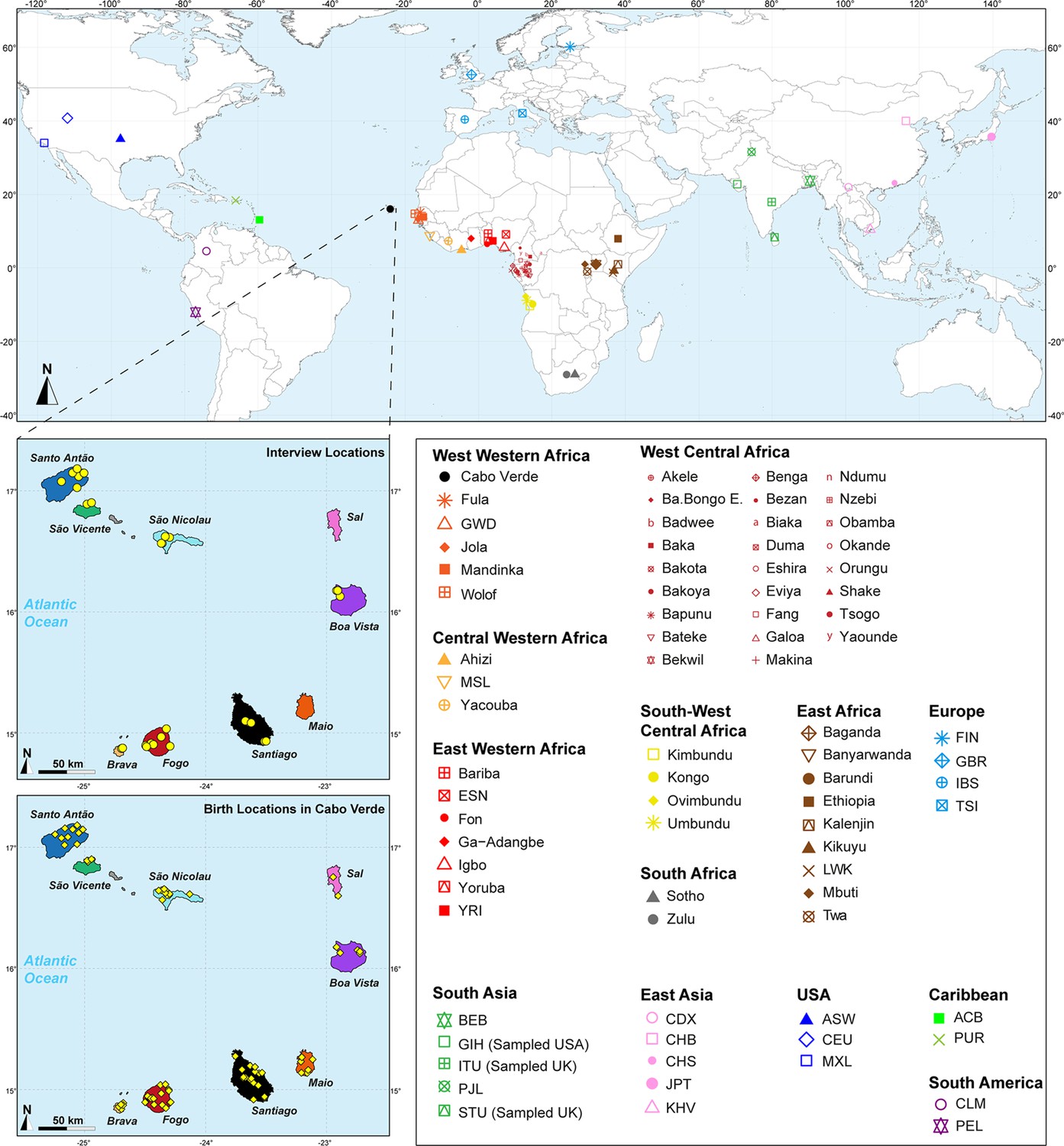
Sampling location of 233 unrelated Cabo Verdean individuals, merged with data on 4924 individuals from 77 worldwide populations.
Birth-location of 225 individuals within Cabo Verde are indicated in the bottom map-panel, and birth locations outside Cabo Verde for 6 individuals are indicated in Figure 1—source data 1. Linguistic and familial anthropology interview, and genetic sampling for Cabo Verde participants were conducted during six separate interdisciplinary fieldworks between 2010 and 2018. Further details about populations are provided in Figure 1—source data 1.
-
Figure 1—source data 1
Population table corresponding to the map in Figure 1 and sample inclusion in all analysis.
- https://cdn.elifesciences.org/articles/79827/elife-79827-fig1-data1-v3.xlsx
Figure 2 with 5 supplements
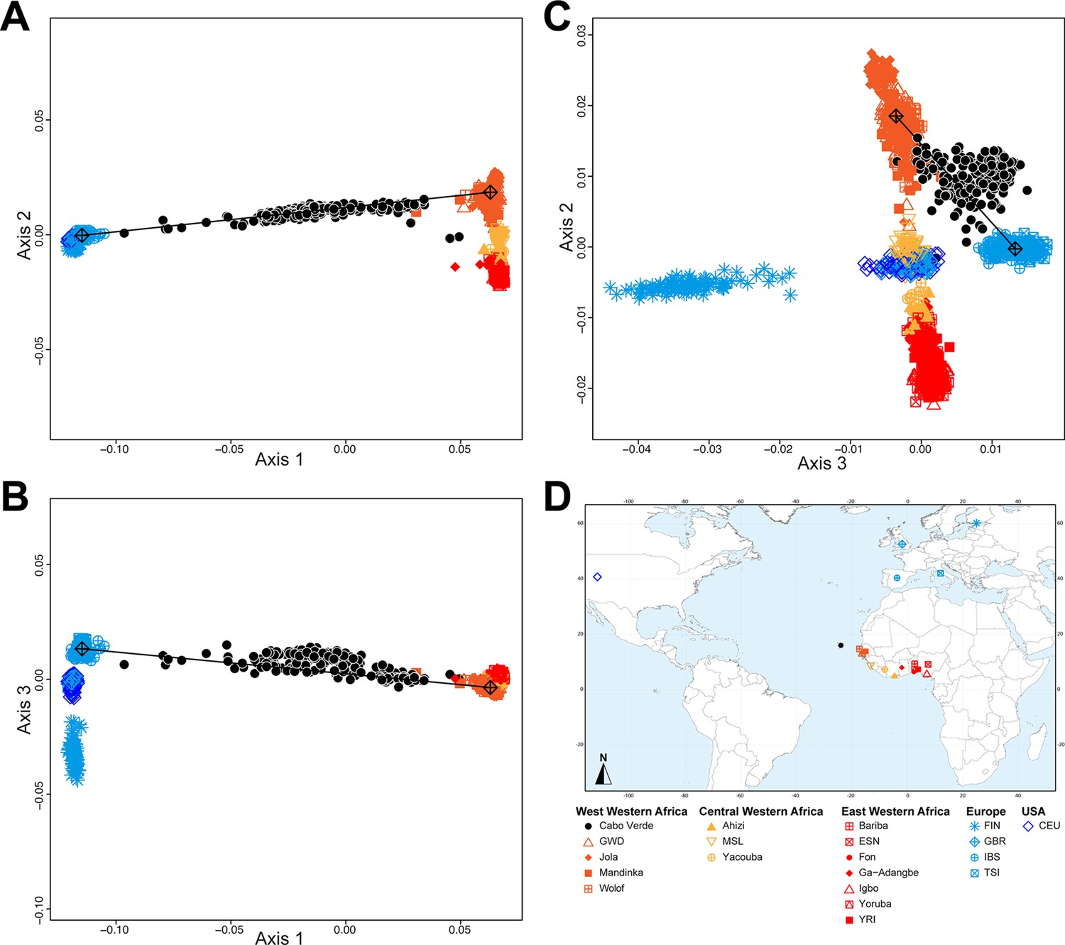
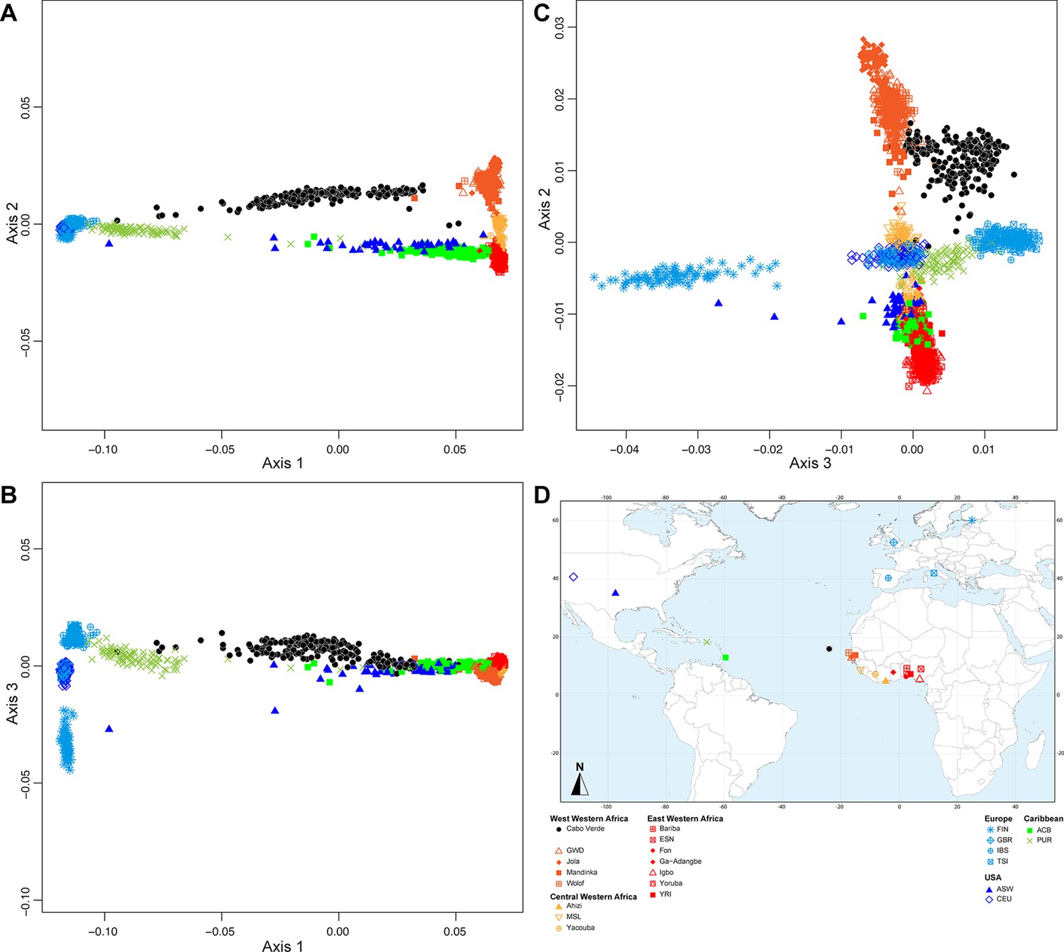
Multidimensional scaling projections of pairwise allele sharing dissimilarities in Cabo Verdeans and continental African and European populations.
(A–C) Three-dimensional MDS projection of ASD computed among 233 unrelated Cabo Verdeans and other continental African and European populations using 445,705 autosomal SNPs. Cabo Verdean patterns in panels A–C can be compared to results obtained considering instead the USA African-Americans ASW, the Barbadians-ACB, and the Puerto Ricans-PUR in the same African and European contexts and presented in Figure 2—figure supplement 1. We computed the Spearman correlation between the matrix of inter-individual three-dimensional Euclidean distances computed from the first three axes of the MDS projection and the original ASD matrix, to evaluate the precision of the dimensionality reduction. We find significant (p<2.2 × 10⁻¹⁶) Spearman ρ=0.9635 for the Cabo Verde analysis (A–C). See Figure 1—source data 1 for the populations used in these analyses. Sample locations and symbols are provided in panel D.
Figure 2—figure supplement 1
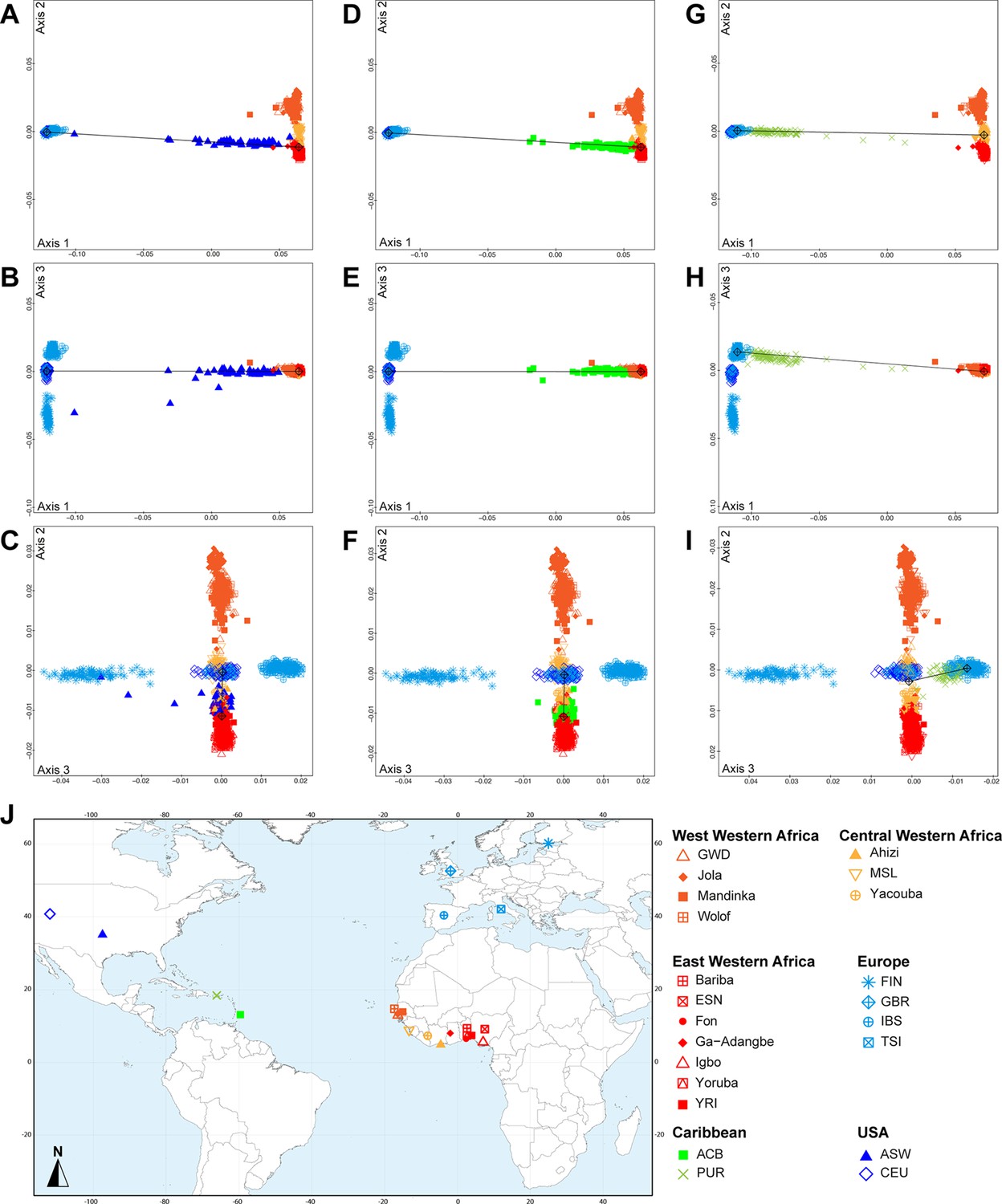
Multidimensional scaling three-dimensional projection of allele sharing pairwise dissimilarities, for the closest subsets of West African and European populations to the African American ASW, Barbadian ACB, and Puerto Rican PUR populations, separately.
Three-dimensional MDS projection of ASD computed using 445,705 autosomal SNPs among continental African and European populations and, respectively, the USA African-American ASW (panels A-C), the Barbadians-ACB (panels D-F), or the Puerto Ricans-PUR (panels G-I), in the same European and African contexts as explored in Figure 2 for Cabo Verdeans in the main text. We computed the Spearman correlation between Euclidean distances on the 3D-MDS projections and the original ASD matrix to evaluate the precision of the dimensionality reduction. We find Spearman ρ=0.9383 (p<2.2 × 10⁻¹⁶) for the ASW (A-C); 0.9306 (p<2.2 × 10⁻¹⁶) for the ACB (D-F); and 0.9437 (p<2.2 × 10⁻¹⁶) for the PUR (G-I). Each individual is represented by a single point. Sample locations and symbols are given in panel J (Figure 1—source data 1).
Figure 2—animation 1
3D animated MDS of pairwise allele sharing dissimilarities in Cabo Verdeans and continental African and European populations.
Figure 2—animation 2
3D animated MDS of pairwise allele sharing dissimilarities in Barbadian ACB and continental African and European populations.
Figure 2—animation 3
3D animated MDS of pairwise allele sharing dissimilarities in Puerto Rican PUR and continental African and European populations.
Figure 2—animation 4
3D animated MDS of pairwise allele sharing dissimilarities in Afro American ASW and continental African and European populations.
Figure 3 with 2 supplements
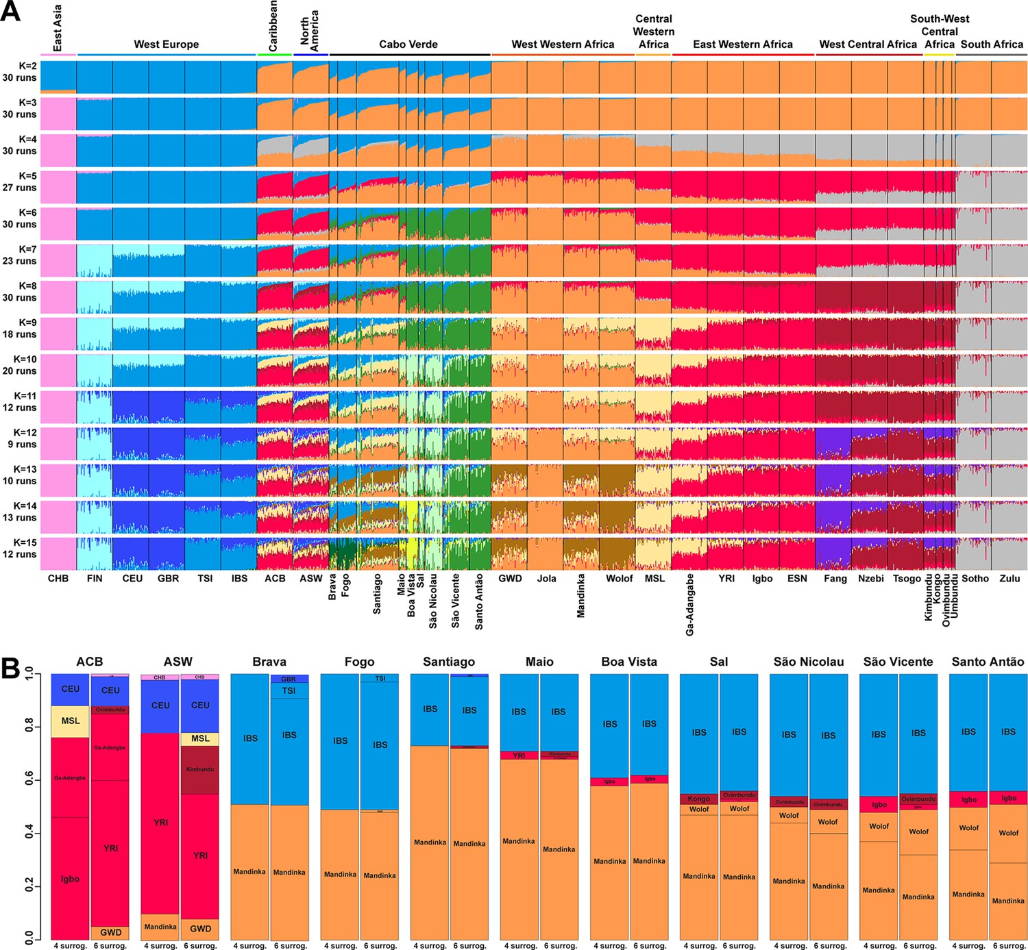
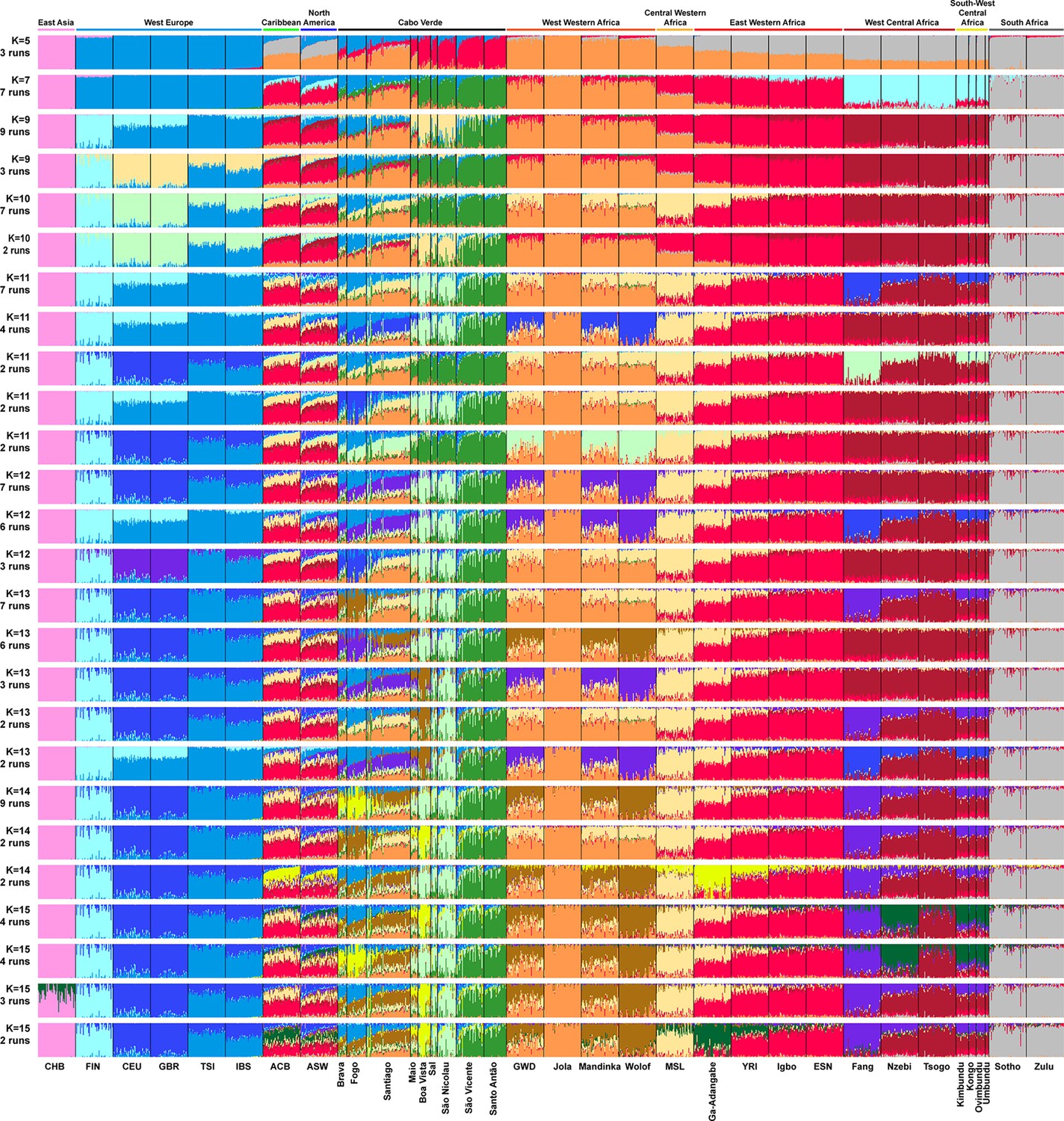
Individual genetic structure and haplotypic local ancestry inference among Cabo Verdean, Barbadian-ACB and African-American ASW populations.
(A) Unsupervised ADMIXTURE analyses using randomly resampled individual sets for populations originally containing more than 50 individuals (Figure 1—source data 1). 225 unrelated Cabo Verdean-born individuals in the analysis are grouped by birth island. Numbers of runs highly resembling one another using CLUMPP are indicated below each K-value. All other modes are presented in Appendix 3—figure 1. (B) SOURCEFIND results for each eleven target admixed populations (ASW, ACB, each of the nine Cabo Verde birth islands), considering respectively 4 or 6 possible source surrogate populations (abbreviated ‘surrog.’) among the 24 possible European, African, and East Asian populations considered in the ADMIXTURE analyses. The cumulated average African admixture levels in each admixed population was highly consistent between SOURCEFIND estimates and ADMIXTURE results at K=2 (Spearman ρ=0.98861, p<2 × 10⁻⁸ and 0.99772, p<8 × 10–12, for 4 or 6 surrogates, respectively). Furthermore, individual admixture levels estimated using an ASD-MDS-based approach (Material and Methods and Appendix 1—figure 2), were highly consistent with individual admixture estimates based on ADMIXTURE results at K=2 (ρ=0.99725; p<2.2 × 10⁻¹⁶ for Cabo Verde; ρ=0.99568; p<2.2 × 10⁻¹⁶ for ASW; ρ=0.99366; p<2.2 × 10⁻¹⁶ for ACB).
Figure 3—figure supplement 1
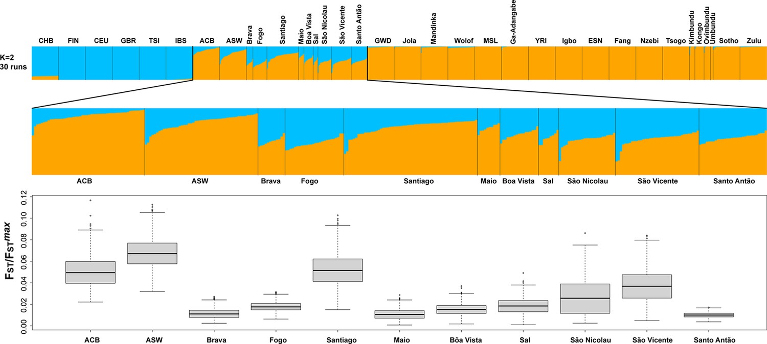
Population Fst/Fstmax values for the ASW, ACB, and each Cabo Verdean birth-island separately considering the ADMIXTURE mode result at K=2 in Figure 3A.
Fst/Fstmax values were computed using FSTruct (Morrison et al., 2022) with 1000 bootstrap replicates per population. All population pairwise distributions of bootstrap Fst/Fstmax values were significantly different from one another after Bonferroni correction (Wilcoxon two-sided rank sum test p<3.96 × 10⁻⁸), except the following pairwise comparisons: ACB-Santiago, Brava-Maio, Fogo-Sal, and Maio-Santo Antão.
Figure 3—figure supplement 2
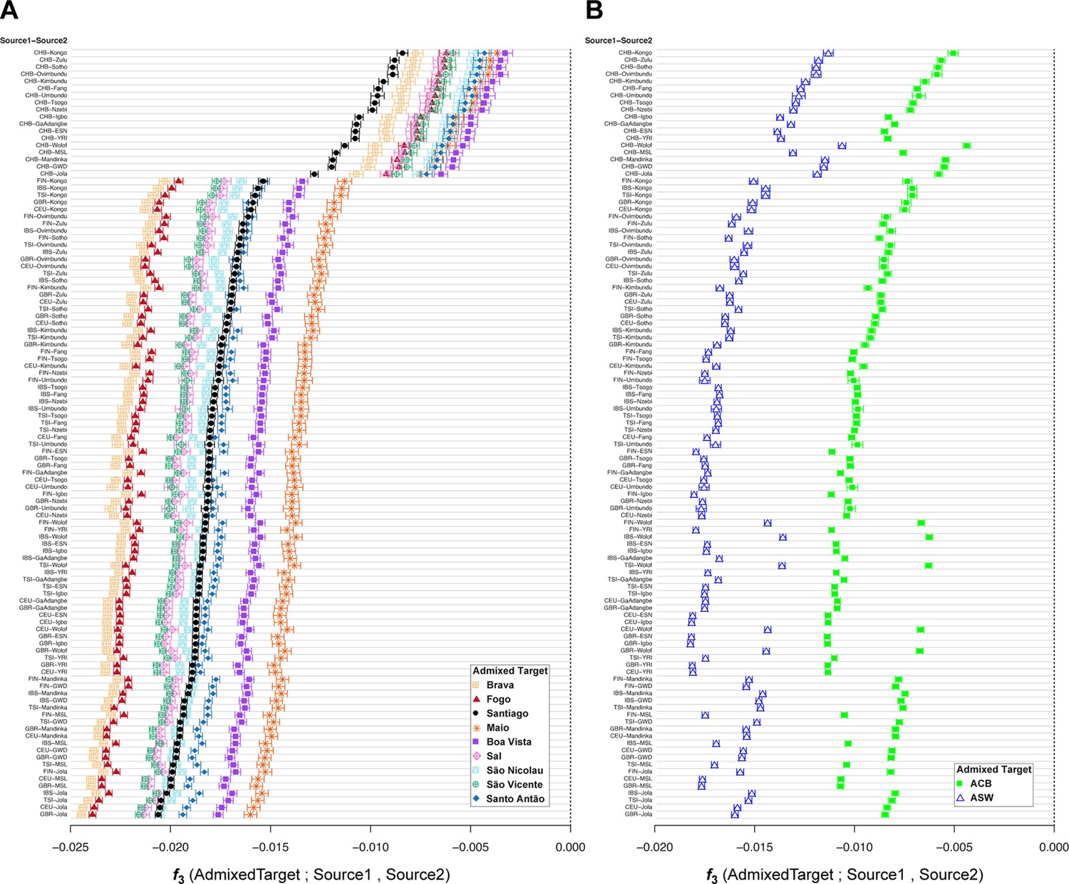
f3-admixture tests of admixture for each Cabo Verdean birth-island, the Barbadian-ACB, and the African-American ASW populations related to the TAST.
As mentioned in the main text of the article, we calculated f3-admixture (Patterson et al., 2012) considering as admixture targets each Cabo Verdean birth-island (panel A), the ASW (panel B), and the ACB (panel B) separately, with, as admixture sources, all 108 possible pairs of one continental European population (Source 1) and one continental African population (Source 2), or the East Asian CHB (Source 1) and one continental African population (Source2), using the same individuals, population groupings, and genotyping dataset as in the previous ADMIXTURE analyses (Figure 1—source data 1). Results for each pair of possible sources are plotted in diminishing values of f3-admixture obtained specifically with Cabo Verde individuals born on Santiago as targets. Target population symbols are indicated in the legend at the bottom-right of each panel.
Figure 4 with 2 supplements
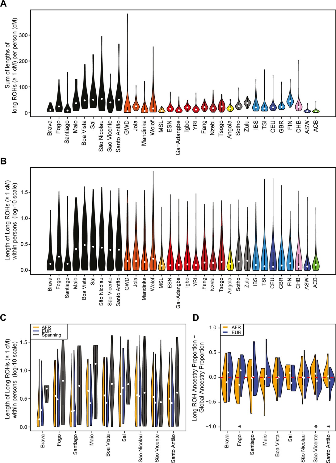
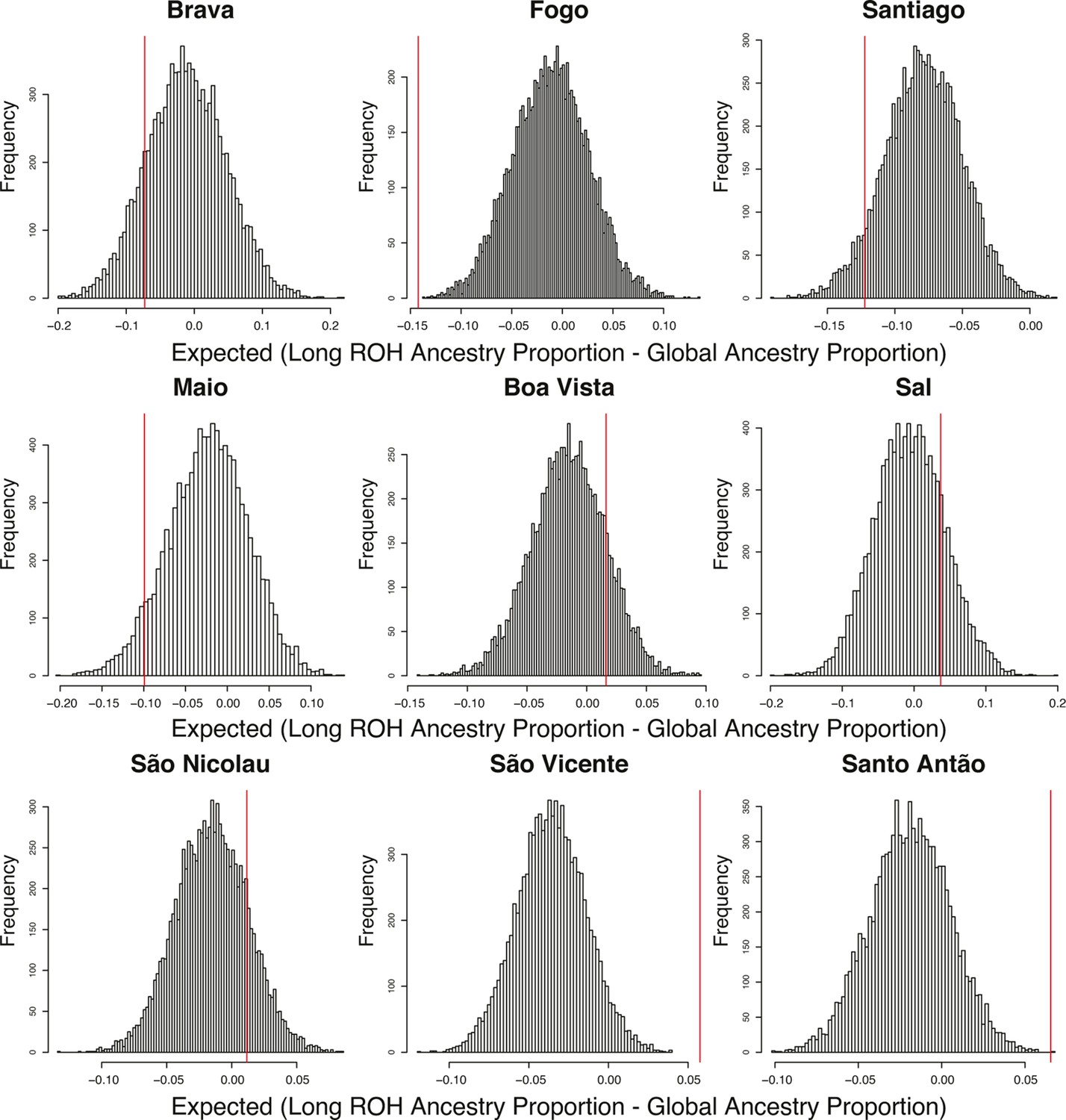
Distributions of long ROHs (≥ 1 cM) in Cabo Verde.
(A) The distribution of the sum of long-ROH (≥1 cM) lengths per person for each Cabo Verdean birth-island and other populations. (B) The length distribution (log-10 scale) of individual long-ROHs identified within samples for each Cabo Verdean birth-island and other populations (e.g. for a distribution with mass at 1.0, this suggests individual ROHs of length 10 cM were identified among samples from that group). (C) The length distribution of ancestry-specific and ancestry-spanning individual long-ROHs for each Cabo Verdean birth-island. (D) The distribution of differences between individuals’ long-ROH ancestry proportion and their global ancestry proportion, for African and European ancestries separately and for each Cabo Verdean birth-island. * indicates significantly (α < 1%) different proportions of ancestry-specific long-ROH, based on non-parametric permutation tests, see Material and Methods, Figure 4—source data 2, and Figure 4—figure supplement 2.
-
Figure 4—source data 1
Mean proportion of total length of ROH that are classified as long (cM ≥1) for each Cabo Verdean island of birth.
- https://cdn.elifesciences.org/articles/79827/elife-79827-fig4-data1-v3.xlsx
-
Figure 4—source data 2
Permutation tests’ p-values for over/under representation of ancestry in long ROH (cM ≥1) for each Cabo Verdean island of birth.
- https://cdn.elifesciences.org/articles/79827/elife-79827-fig4-data2-v3.xlsx
-
Figure 4—source data 3
Mean proportion of total length of long ROH (cM ≥1) that have heterozygous ancestry (AFR and EUR), for each Cabo Verdean island of birth.
- https://cdn.elifesciences.org/articles/79827/elife-79827-fig4-data3-v3.xlsx
Figure 4—figure supplement 1
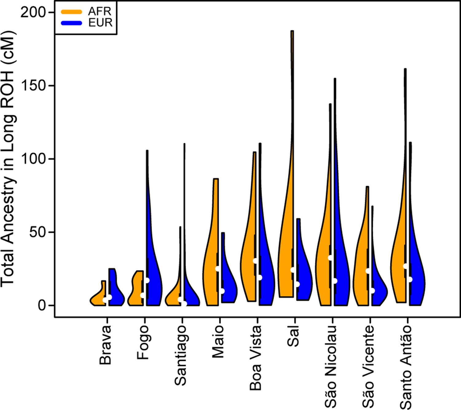
The distribution of total ancestry in long ROH per individual for each Cabo Verdean birth-island.
Figure 4—figure supplement 2
Permutation distributions for over/under representation of ancestry in long ROH (≥1 cM) for each Cabo Verdean island of birth.
As mentioned in Material and Methods, for each individual in each island, we randomly permuted the location of all long ROH (ensuring that no permuted ROH overlap), re-computed the local AFR ancestry proportion falling within these permuted ROH, and then subtracted the global ancestry proportion. We then take the mean of this difference across all individuals for each island and repeat the process 10,000 times. As there is negligible ASN ancestry across these individuals, the AFR and EUR proportions essentially add to 1, and therefore we consider an over/under representation of AFR ancestry in long ROH to be equivalent to an under/over representation of EUR ancestry in long ROH. Observed values in the real data set are provided as a red vertical line for each island of birth separately. Permutation p-values are reported in Figure 4—source data 2.
Figure 5
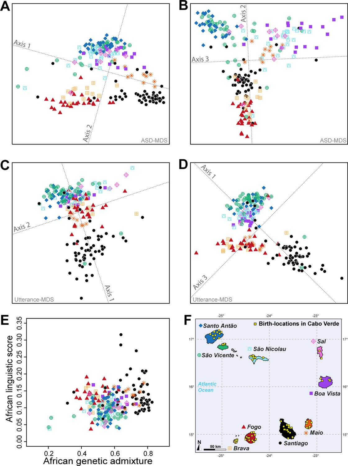
Utterance and genetic diversity and admixture within Cabo Verde.
(A–B) 3D MDS projection of Allele Sharing Dissimilarities computed among 225 unrelated Cabo-Verde-born individuals using 1,899,878 autosomal SNPs. Three-dimensional Euclidean distances between pairs of individuals in this MDS significantly correlated with ASD (Spearman ρ=0.6863; p<2.2 × 10⁻¹⁶). (C–D) 3D MDS projection of individual pairwise Euclidean distances between uttered linguistic items frequencies based on the 4831 unique uttered items obtained from semi-spontaneous discourses. Three-dimensional Euclidean distances between pairs of individuals in this MDS significantly correlated with the utterance-frequencies distances (Spearman ρ=0.8647; p<2.2 × 10⁻¹⁶). (E) Spearman correlation ρ=0.2070 (p=0.0018) between individual African utterance scores and individual genetic African admixture rates obtained with ADMIXTURE at K=2. (F) Birth-locations of 225 individuals in Cabo Verde. Symbols for individuals’ birth-island in panels A–E are shown in panel F. Panel A–D were Procrustes-transformed according to individual actual birth-places’ geographical locations in panel F (Wang et al., 2010).
Figure 6
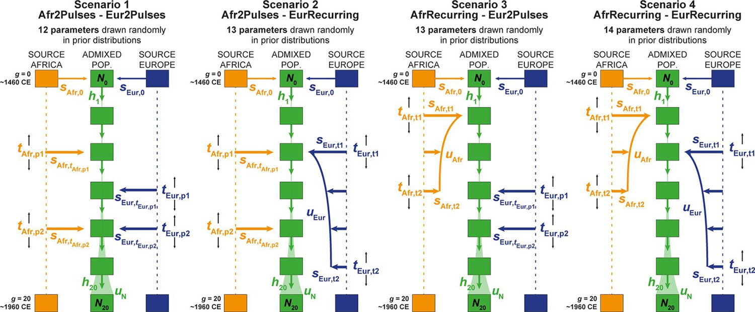
Four competing scenarios for the genetic admixture histories of each Cabo Verde island.
For all scenarios, the duration of the admixture process is set to 20 generations after the initial founding admixture event occurring at generation 0, which corresponds roughly to the initial peopling of Cabo Verde in the 1460s, considering 25 years per generation and sampled individuals born on average between the 1960s and 1980s. Scenario 1 Afr2Pulses-Eur2Pulses: after the initial founding pulse of admixture, the admixed population receives two separate introgression pulses from the African and European sources, respectively. Scenario 2 Afr2Pulses-EurRecurring: after the initial founding pulse of admixture, the admixed population receives two separate introgression pulses from the African source, and a period of monotonically constant or decreasing recurring introgression from the European source. Scenario 3 AfrRecurring-Eur2Pulses: after the initial founding pulse of admixture, the admixed population receives a period of monotonically constant or decreasing recurring introgression from the African source, and two separate introgression pulses from the European source. Scenario 4 AfrRecurring-EurRecurring: after the initial founding pulse of admixture, the admixed population receives a period of monotonically constant or decreasing recurring introgression from the African source, and, separately, a period of monotonically constant or decreasing recurring introgression from the European source. For all scenarios, we consider demographic models corresponding to either a constant reproductive population size Ng between the founding event and the present, or, instead, a linear or hyperbolic increase between N0 and N20, depending on the values of N0, N20, and uN used for each simulation respectively. Time for admixture pulses or time for the onset and offset of admixture periods are schematically represented as tSource,g. We define (Verdu and Rosenberg, 2011), sAfr,g, sEur,g, and hg as the proportion of parents of individuals in the admixed population at generation g coming from, respectively, the African source population, the European one, and the admixed population itself at the previous generation. Thus, for g=0, sAfr,0 + sEur,0 = 1, and for each value of g in [1,20], sAfr,g + sEur,g+ hg = 1. The number of ‘free’ scenario-parameters drawn randomly in prior distributions set by the user for simulations and subsequent Approximate Bayesian Computation inferences is indicated below the name of each scenario respectively. See Table 2 for parameter prior distributions, and Material and Methods for detailed descriptions of scenario-parameters.
Figure 7 with 3 supplements
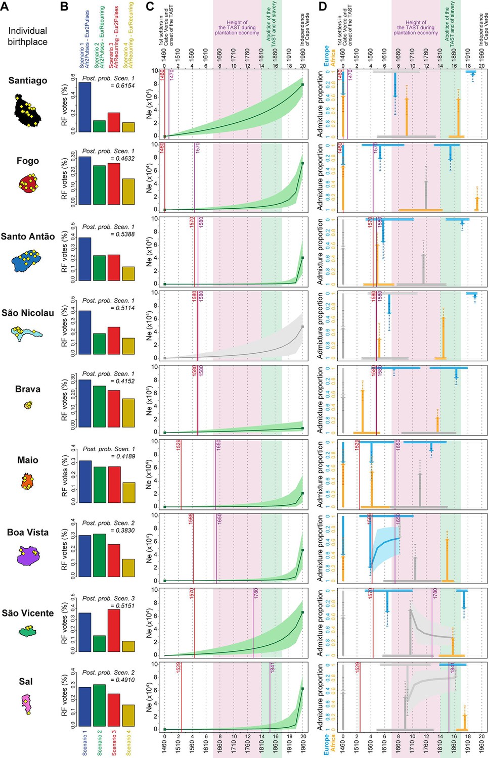
Genetic admixture histories of Cabo Verde islands inferred with MetHis-Approximate Bayesian Computation.
Elements of the peopling-history of Cabo Verde islands are synthesized in Figure 7—source data 1, stemming from historical work cited therein. Islands are ordered from top to bottom in the chronological order of the first historical census perennially above 100 individuals within an island, indicated with the purple vertical lines. First historical records of the administrative, political, and religious, settlement of an island, are indicated with the red vertical lines. (A) Within-island birth-places of 225 Cabo-Verde-born individuals. (B) MetHis-Random Forest-ABC scenario-choice vote results for each island separately in histogram format. Posterior probabilities of correctly identifying a scenario if correct are indicated for the winning scenario as ‘Post. prob. Scen.’, above each histogram. (C) MetHis-Neural Network-ABC posterior parameter distributions with 50% Credibility Intervals for the reproductive population size history of each birth-island separately. (D) Synthesis of MetHis-NN-ABC posterior parameter median point-estimates and associated 50% CI, for the admixture history of each island under the winning scenario identified with RF-ABC in panel B. European admixture history appears in blue, African admixture history in orange. Horizontal bars indicate 50% CI for the admixture time parameters, vertical arrows correspond to median admixture intensity estimates with 50% CI in doted lines. For (C) and (D), posterior parameter distributions showing limited departure from their respective priors and large CI are greyed, as they were largely unidentifiable in our ABC procedures. Detailed parameter posterior distributions, 95% CI, and cross-validation errors are provided in Figure 7—figure supplements 1–3 and Appendix 5—Tables 1–9. Detailed results description for each island are provided in Appendix 5. (C–D) The period between the 1630s and the abolition of the TAST in the 1810s, when most enslaved-Africans were deported from Africa by European empires concomitantly to the expansion of the plantation economy (Eltis and Richardson, 2015; Fortes-Lima and Verdu, 2021), is indicated in light-pink. The period between the abolition of the TAST in the 1810s and the abolition of slavery enacted between 1856 and 1878 throughout the Portuguese empire is indicated in light-green (Carreira, 2000). The independence of Cabo Verde occurred in 1975.
-
Figure 7—source data 1
Historical landmark chronology for the peopling history of Cabo Verde as provided by previous historical work, respectively for each island.
- https://cdn.elifesciences.org/articles/79827/elife-79827-fig7-data1-v3.xlsx
Figure 7—figure supplement 1
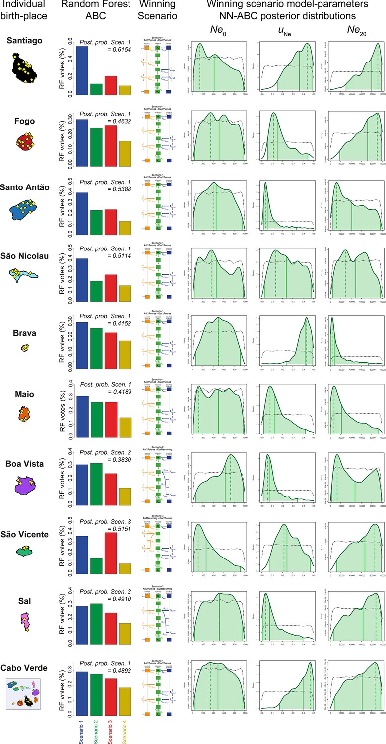
Reproductive-size posterior parameter distributions and associated priors obtained with Neural Network ABC inference for each island separately.
We considered, for each island separately, and for all 225 Cabo Verde-born individuals grouped in a single random mating population separately, Neural Network tolerance levels and number of neurons in the hidden layer, for each island and for Cabo Verde as a whole, separately, are chosen based on posterior parameter cross-validation error minimization procedures conducted on 1000 random simulations used in-turn, as pseudo observed data (see Appendix 1, and Appendix 1—table 1). For each island and for Cabo Verde as a whole, separately, posterior parameter distributions correspond to the solid lines and corresponding priors correspond to the doted black lines. Density distributions are based on the logit transformation of parameter values (see Appendix 1) using an Epanechnikov kernel between the corresponding prior bounds. See Results, Discussion, and Appendix 5 for descriptions and discussions of the results. Synthesis in Figure 7.
Figure 7—figure supplement 2
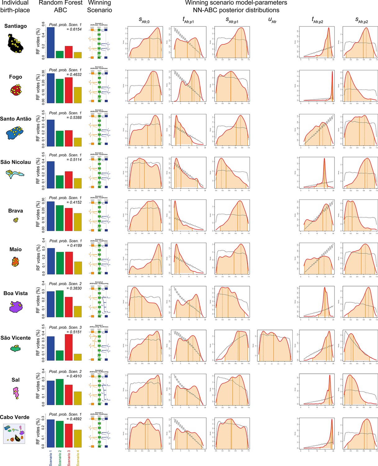
African admixture histories posterior parameter distributions and associated priors obtained with Neural Network ABC inference for each island separately.
We considered, for each island separately, and for all 225 Cabo Verde-born individuals grouped in a single random mating population separately, Neural Network tolerance levels and number of neurons in the hidden layer, for each island and for Cabo Verde as a whole, separately, are chosen based on posterior parameter cross-validation error minimization procedures conducted on 1000 random simulations used in-turn, as pseudo observed data (see Appendix 1, and Appendix 1—table 1). For each island and for Cabo Verde as a whole, separately, posterior parameter distributions correspond to the solid lines and corresponding priors correspond to the doted black lines. Density distributions are based on the logit transformation of parameter values (see Appendix 1) using an Epanechnikov kernel between the corresponding prior bounds. See Results, Discussion, and Appendix 5 for descriptions and discussions of the results. Synthesis in Figure 7.
Figure 7—figure supplement 3
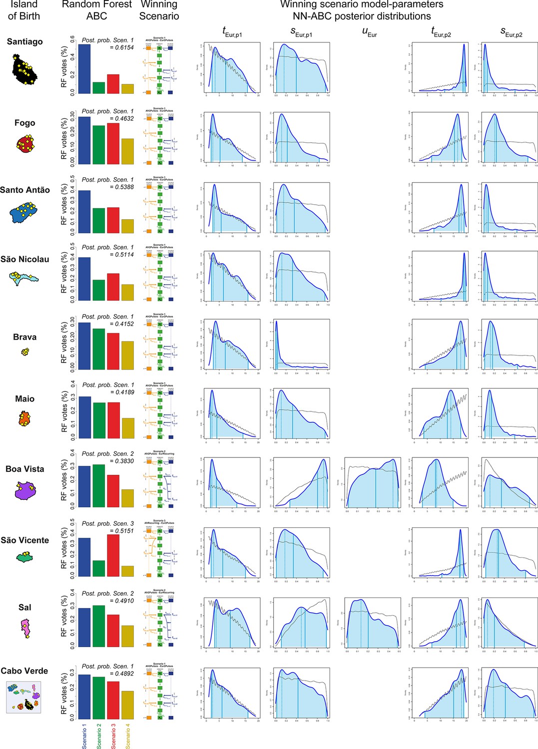
European admixture histories posterior parameter distributions and associated priors obtained with Neural Network ABC inference for each island separately.
We considered, for each island separately, and for all 225 Cabo Verde-born individuals grouped in a single random mating population separately, 100,000 simulations computed under the winning scenario obtained with RF-ABC scenario-choice procedures and provided on the left of the figure. Neural Network tolerance levels and number of neurons in the hidden layer, for each island and for Cabo Verde as a whole, separately, are chosen based on posterior parameter cross-validation error minimization procedures conducted on 1000 random simulations used in-turn, as pseudo observed data (see Appendix 1, and Appendix 1—table 1). For each island and for Cabo Verde as a whole, posterior parameter distributions correspond to the solid lines and corresponding priors correspond to the doted black lines. Density distributions are based on the logit transformation of parameter values (see Appendix 1) using an Epanechnikov kernel between the corresponding prior bounds. See Results, Discussion, and Appendix 5 for descriptions and discussions of the results. Synthesis in Figure 7.
Appendix 1—figure 1
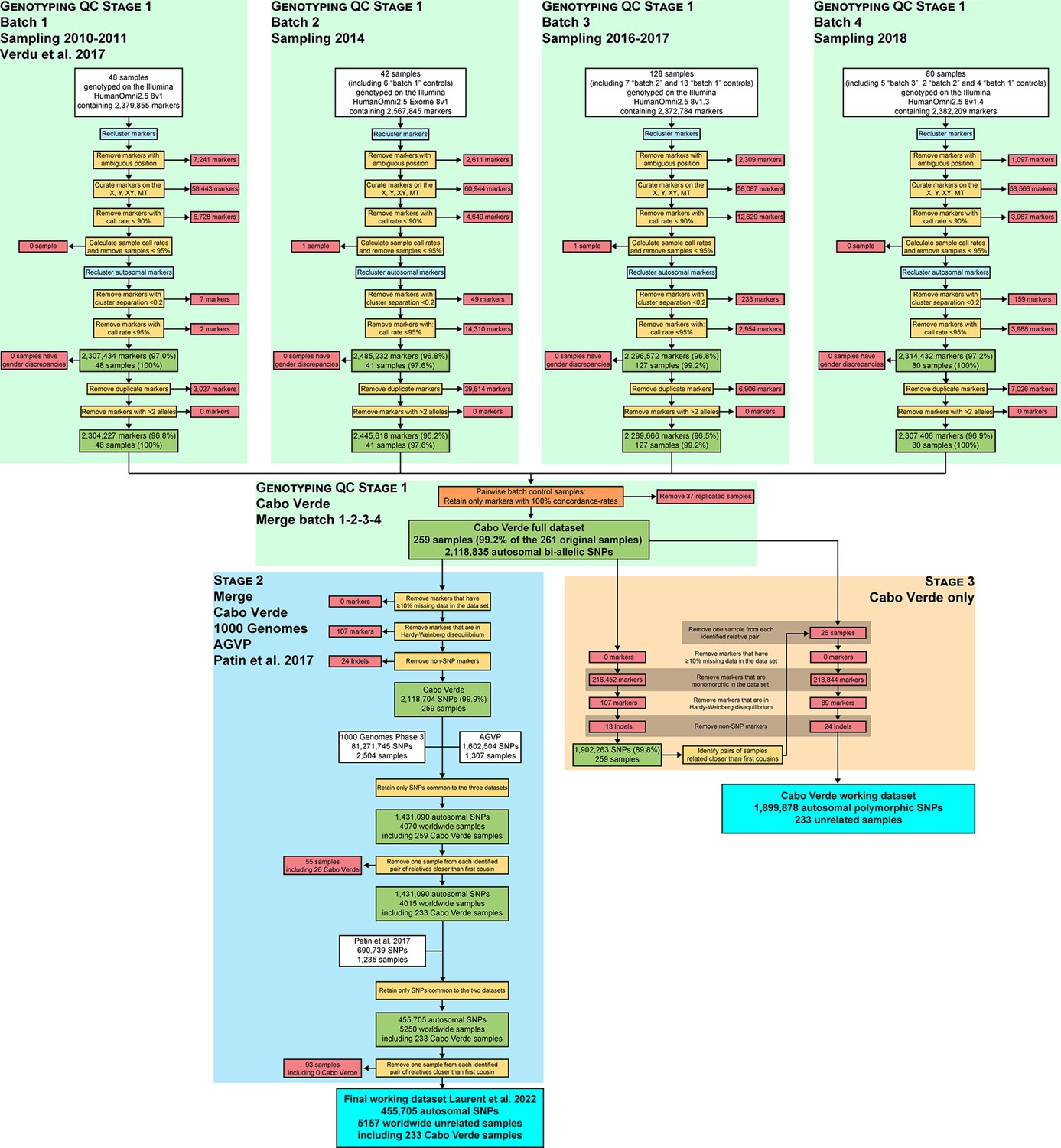
Quality-control and datasets merging procedures.
Quality controls at the genotyping call level (Stage 1) were conducted with Illumina’s GenomeStudio software Genotyping Module. Cabo Verde original DNA samples have been collected during six separate field-trips between 2010 and 2018, genotyped in four batches using four different versions of the Illumina Omni2.5Million Beadchip genotyping array. The resulting dataset was merged with 2,504 worldwide samples from the 1000 Genomes Project Phase 3 Auton et al., 2015; with 1,307 continental African samples from the African Genome Variation Project (EGA accession number EGAD00001000959, Gurdasani et al., 2015); and with 1,235 African samples from Patin et al., 2017 (EGA accession number EGAS00001002078). We retained only autosomal SNPs common to all datasets, and excluded one individual for each pair of individuals related at the 2nd degree (at least one grand-parent in common) as inferred with KING (Manichaikul et al., 2010), following previous procedures (Verdu et al., 2017).
Appendix 1—figure 2
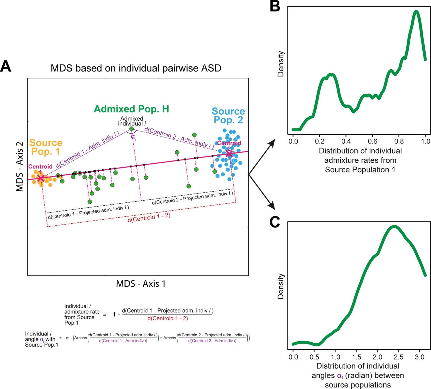
Schematic representation of the ASD-MDS estimates of individual admixture proportions and angles, also used as summary statistics for ABC inference and implemented in MetHis summary-statistic calculation tools.
All the panels of the figure are schematic.
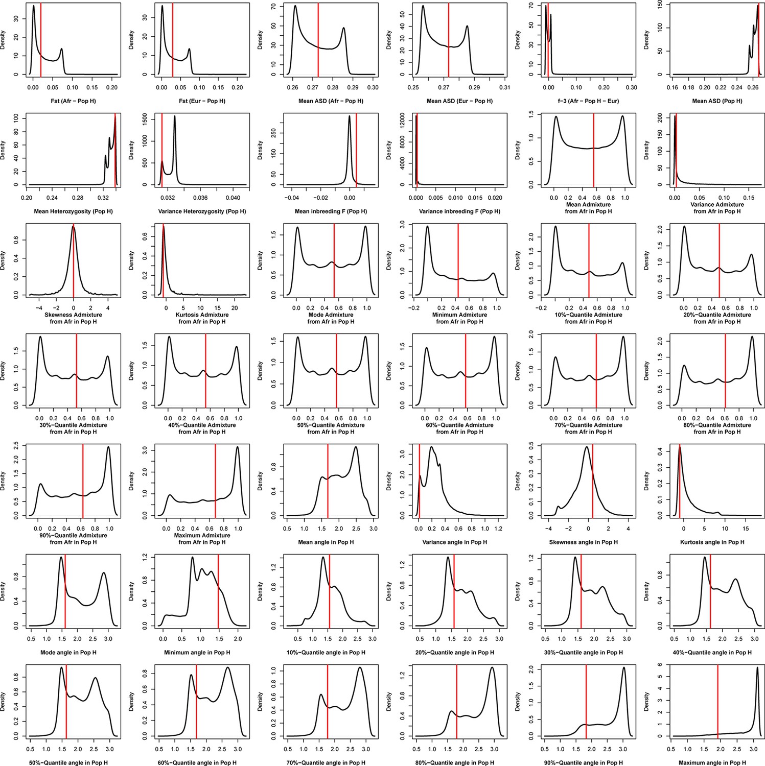
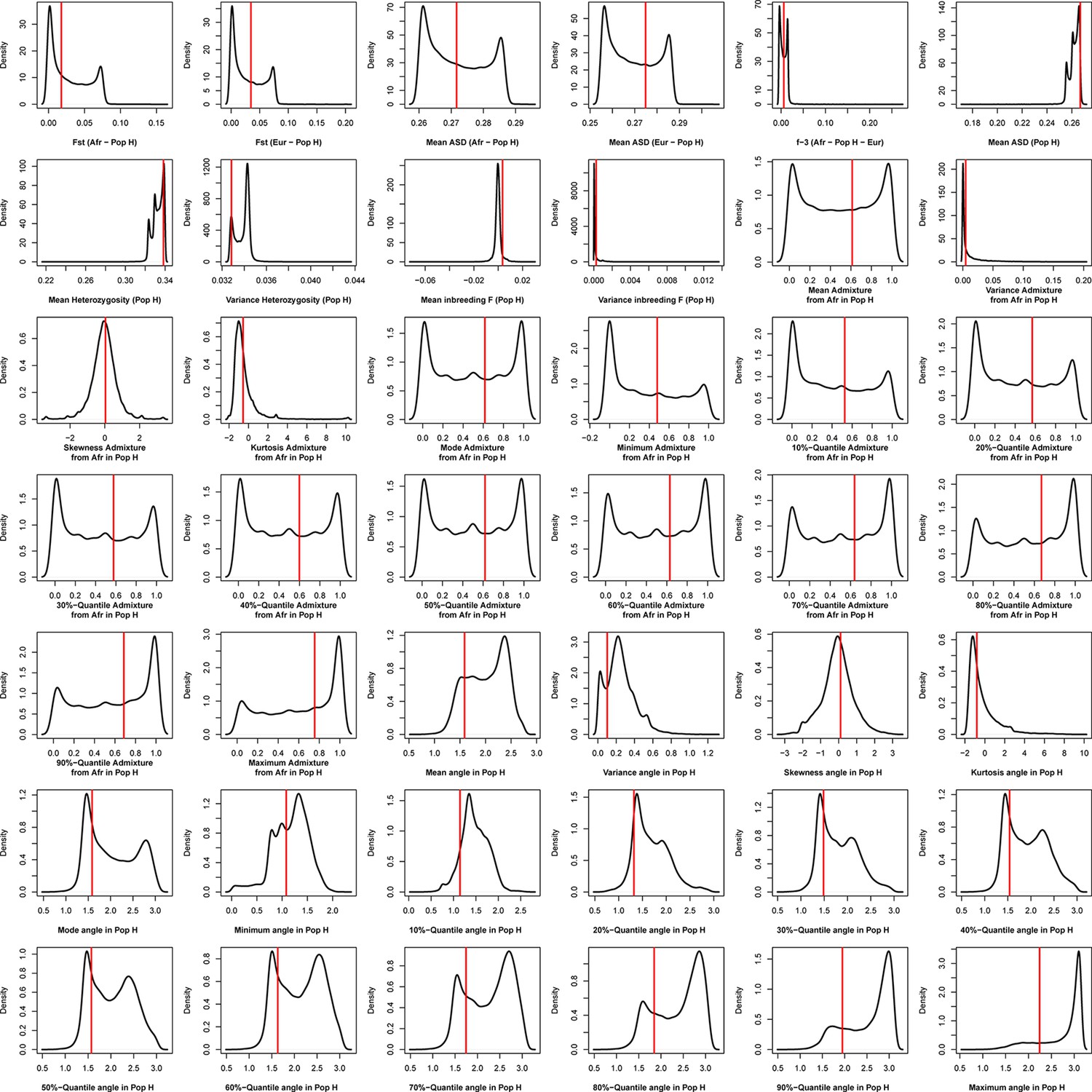
Appendix 1—figure 3 with 10 supplements
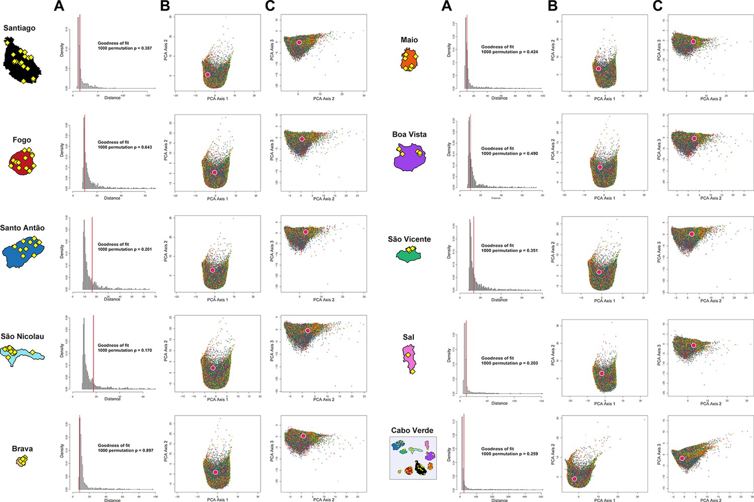
ABC Prior-checking for MetHis simulations for each island separately.
10,000 simulations are conducted under each four competing scenarios of historical admixture considered in Random-Forest ABC scenario-choice (see Figure 6). (A) Goodness-of-Fit tests: we use as goodness-of-fit statistic the median of the distance between one target vector of 42 summary-statistics and the vectors of 42 statistics obtained for the 1% simulations in the 40,000 simulations reference table that are closest to the target (as identified by simple rejection Pritchard et al., 1999). Results obtained with the observed data as target are indicated in the vertical red line. Null-distribution of the goodness-of-fit statistics as histograms are obtained by considering as target in-turn 1000 random simulations as pseudo-observed data, for each island and for the 225 Cabo Verde-born individuals grouped in a single random-mating population, separately. (B) First two axes of a principal component analysis performed on the 42 summary-statistics obtained for 40,000 simulations per island (10,000 simulations for each of four competing-scenarios). Each point corresponds to a single simulation colored per scenario: simulations under Scenario 1 are in blue; Scenario 2 in green; Scenario 3 in red; and Scenario 4 in yellow (Figures 6–7). The pink white-circled dot corresponds to the vector of summary-statistics from the observed dataset. (C) Axes 1 and 3 of the same PCA projection as in panel B.
Appendix 1—figure 3—figure supplement 1
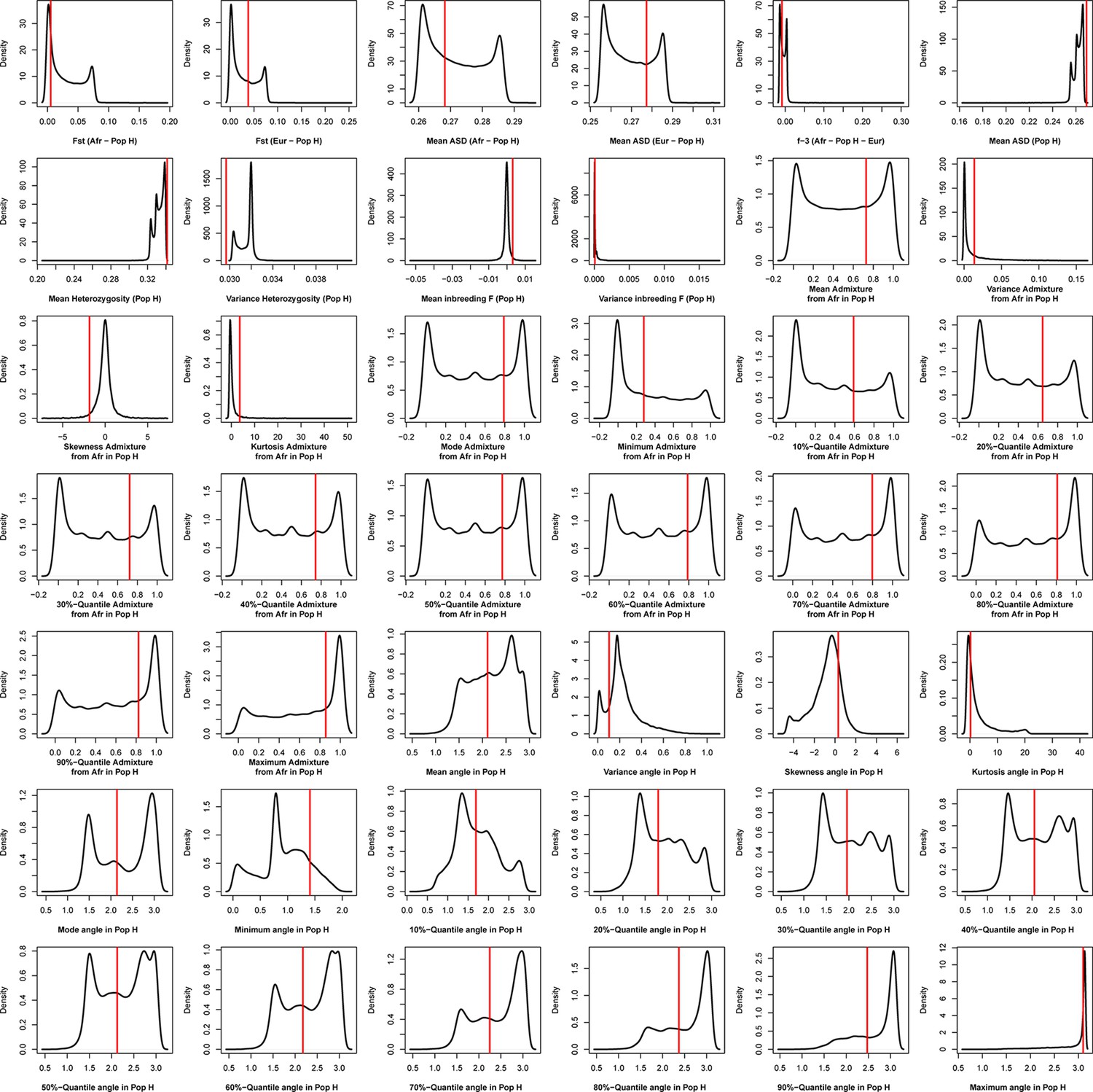
Density distributions (black line) of each of 42 summary-statistics obtained from 40,000 simulations, 10,000 under each of four competing scenarios for Santiago, compared to the observed statistic obtained in this island (red vertical line).
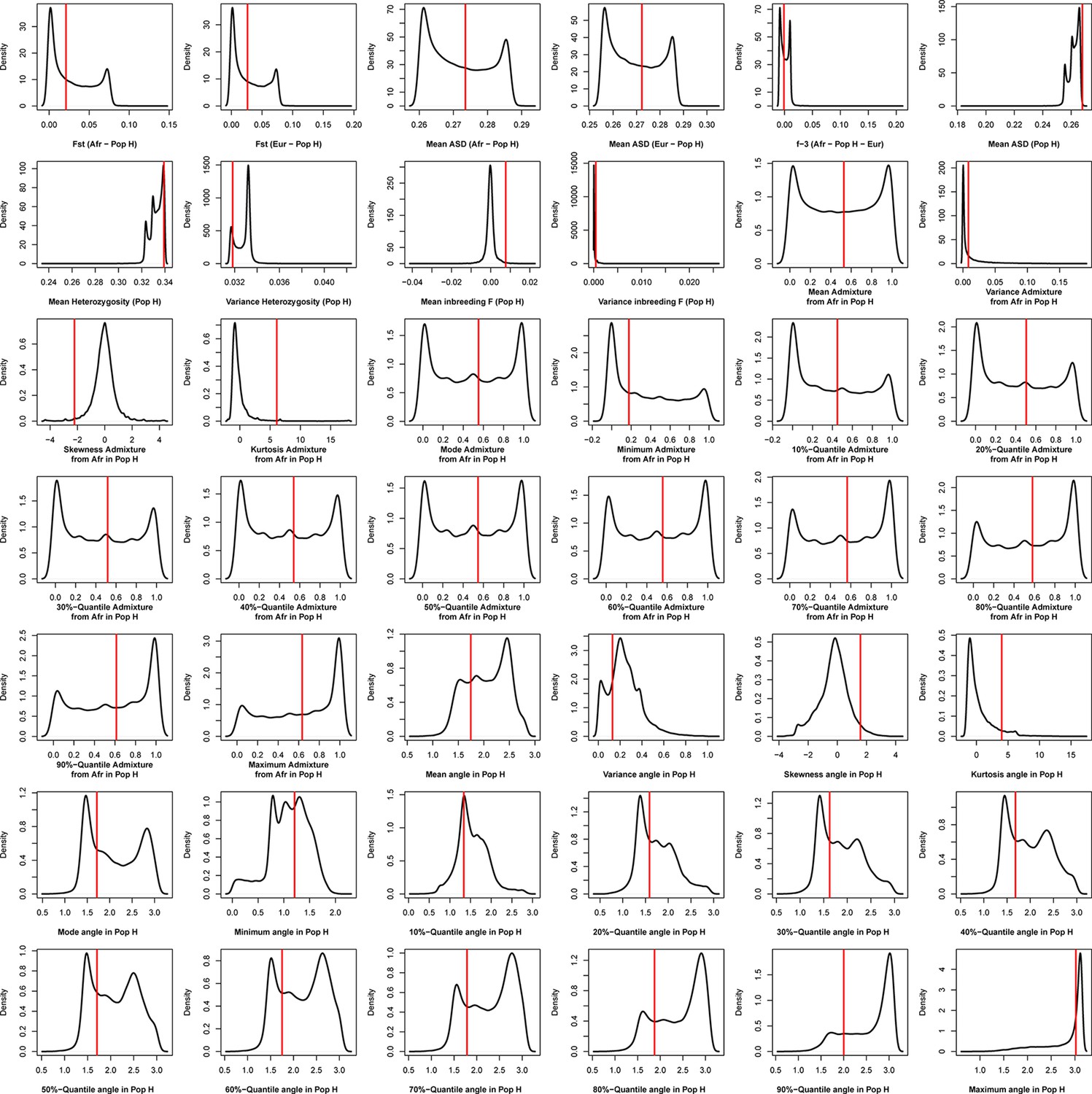
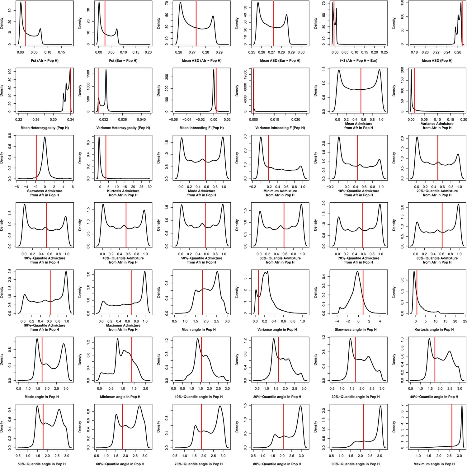
Appendix 1—figure 3—figure supplement 2
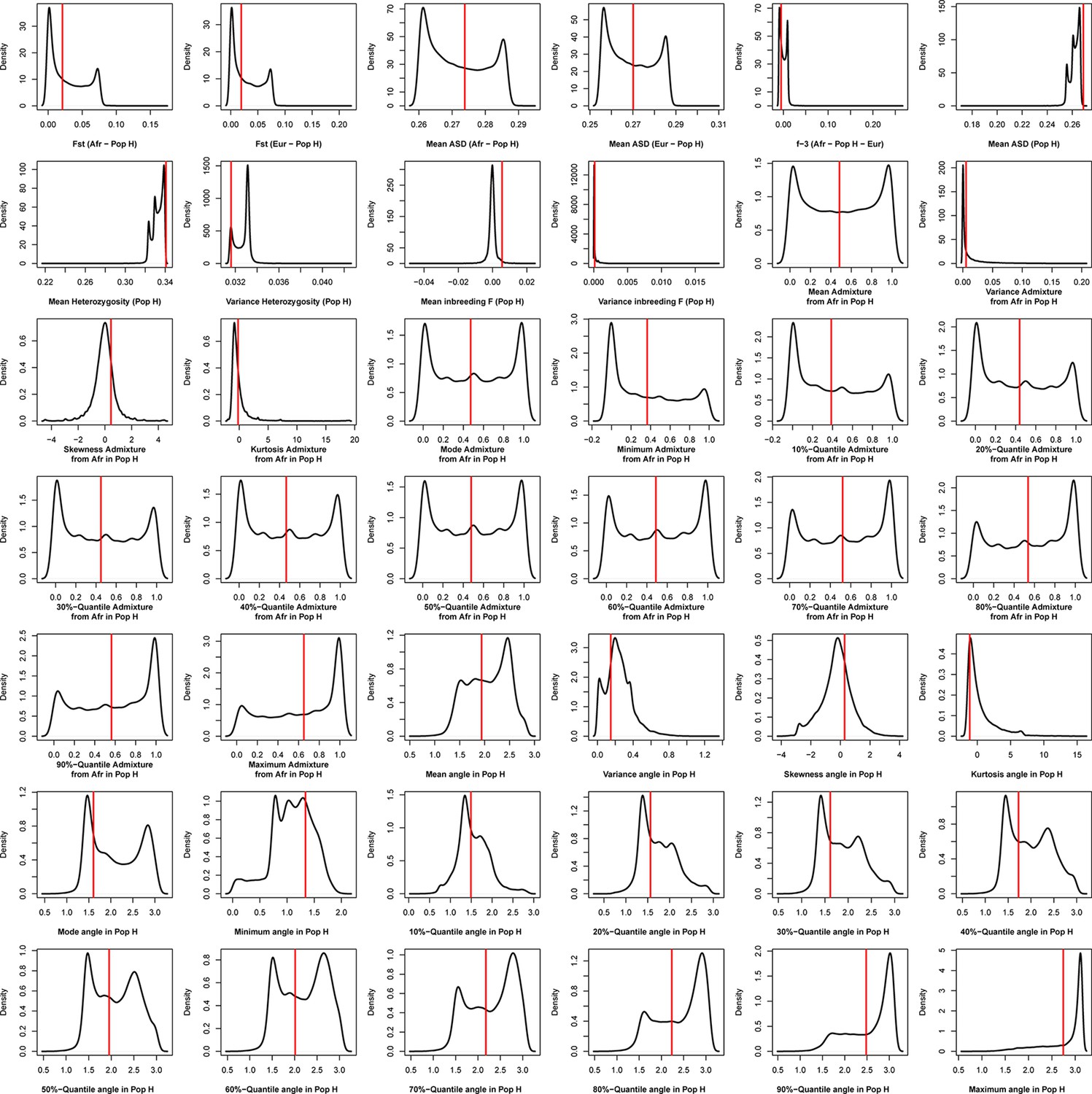
Density distributions (black line) of each of 42 summary-statistics obtained from 40,000 simulations, 10,000 under each of four competing scenarios for Fogo, compared to the observed statistic obtained in this island (red vertical line).
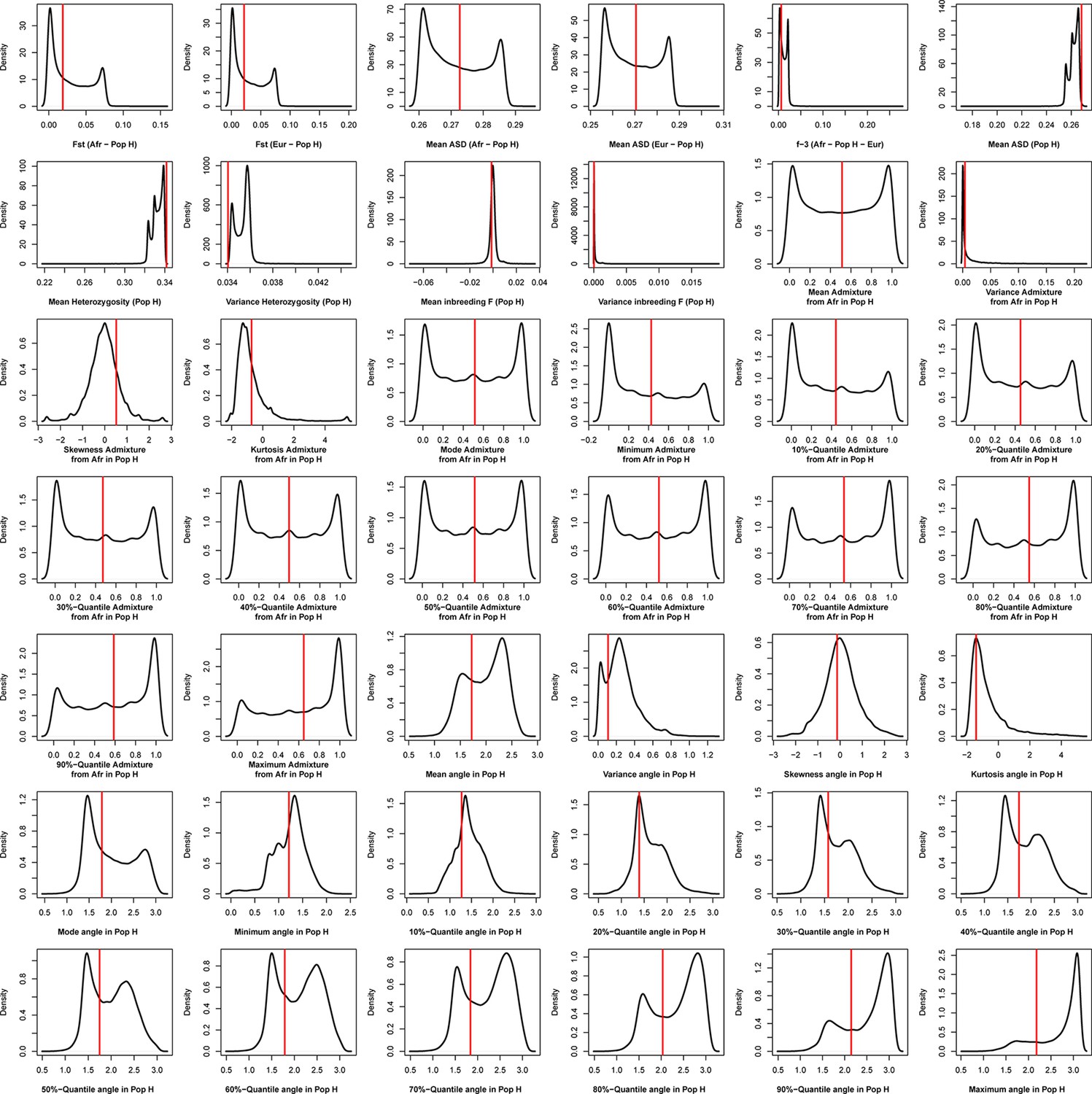
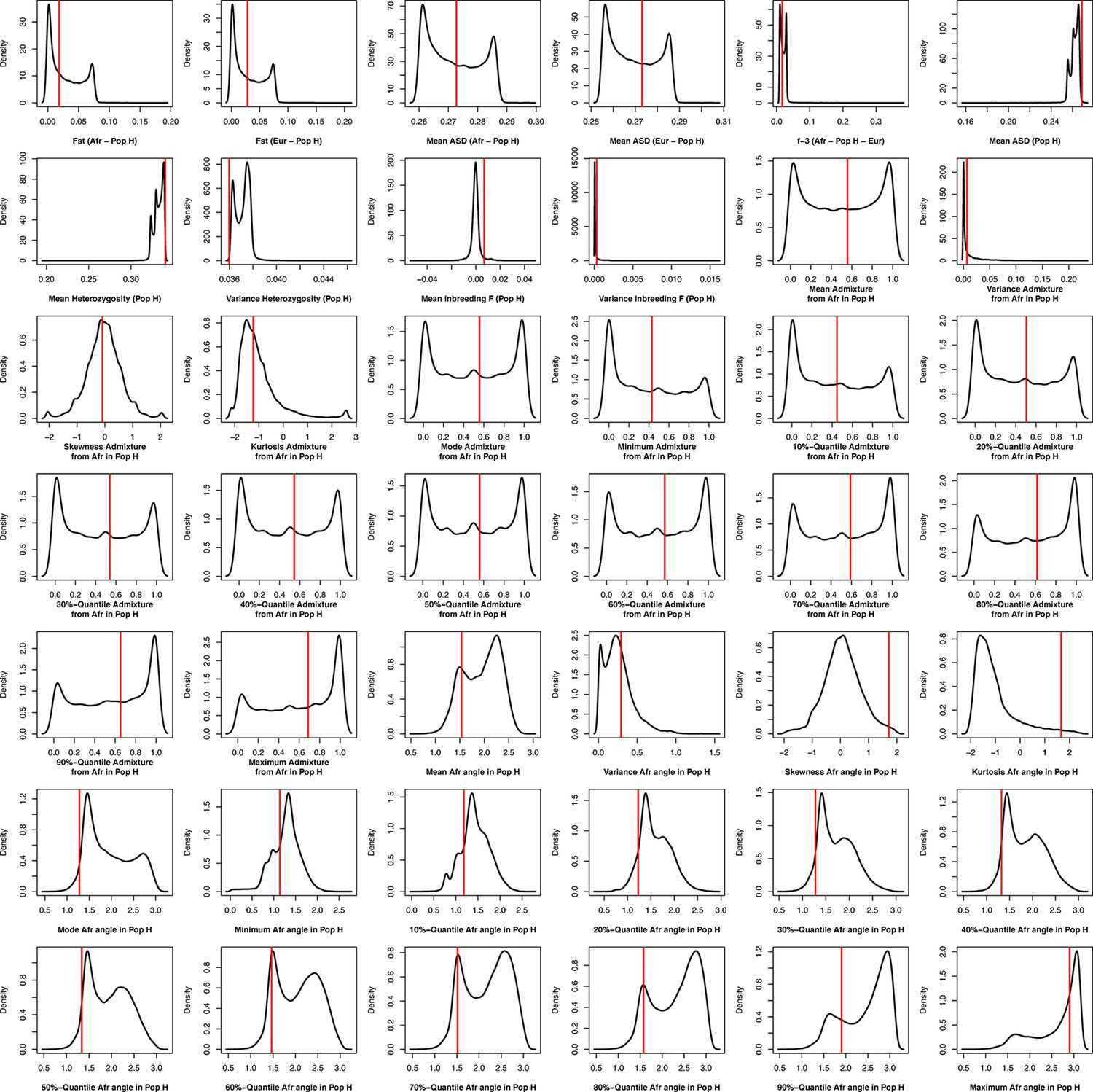
Appendix 1—figure 3—figure supplement 3
Density distributions (black line) of each of 42 summary-statistics obtained from 40,000 simulations, 10,000 under each of four competing scenarios for Santo Antão, compared to the observed statistic obtained in this island (red vertical line).The four scenarios are synthetically described in Figure 6 and the 42 summary-statistics in Table 3.
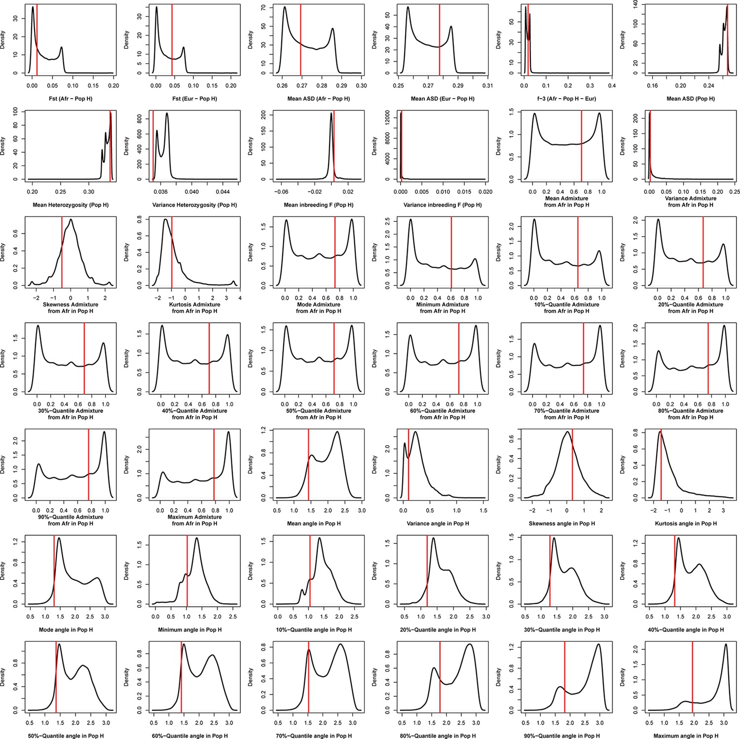
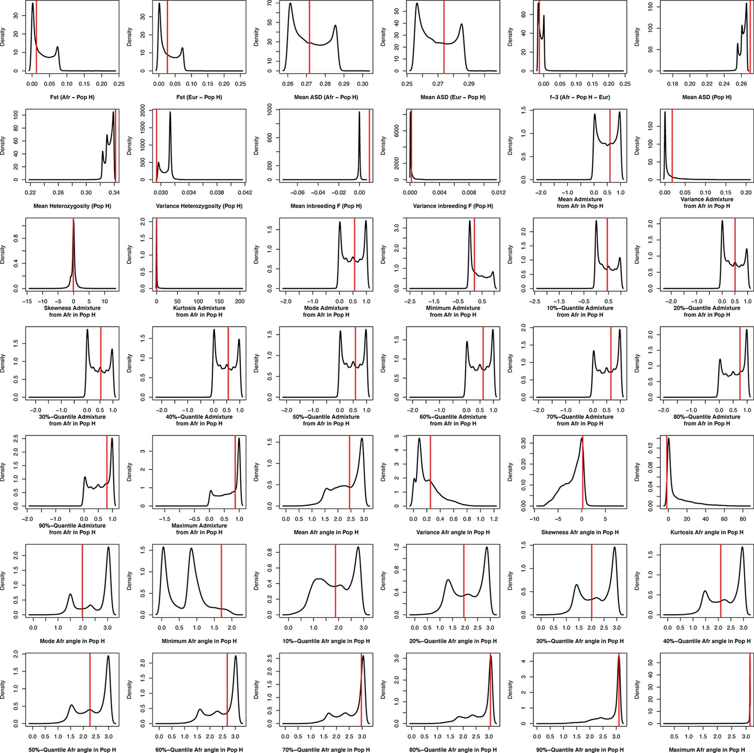
Appendix 1—figure 3—figure supplement 4
Density distributions (black line) of each of 42 summary-statistics obtained from 40,000 simulations, 10,000 under each of four competing scenarios for São Nicolau, compared to the observed statistic obtained in this island (red vertical line).
Appendix 1—figure 3—figure supplement 5
Density distributions (black line) of each of 42 summary-statistics obtained from 40,000 simulations, 10,000 under each of four competing scenarios for Brava, compared to the observed statistic obtained in this island (red vertical line).
Appendix 1—figure 3—figure supplement 6
Density distributions (black line) of each of 42 summary-statistics obtained from 40,000 simulations, 10,000 under each of four competing scenarios for Maio, compared to the observed statistic obtained in this island (red vertical line).
Appendix 1—figure 3—figure supplement 7
Density distributions (black line) of each of 42 summary-statistics obtained from 40,000 simulations, 10,000 under each of four competing scenarios for Boa Vista, compared to the observed statistic obtained in this island (red vertical line).
Appendix 1—figure 3—figure supplement 8
Density distributions (black line) of each of 42 summary-statistics obtained from 40,000 simulations, 10,000 under each of four competing scenarios for São Vicente, compared to the observed statistic obtained in this island (red vertical line).
Appendix 1—figure 3—figure supplement 9
Density distributions (black line) of each of 42 summary-statistics obtained from 40,000 simulations, 10,000 under each of four competing scenarios for Sal, compared to the observed statistic obtained in this island (red vertical line).
Appendix 1—figure 3—figure supplement 10
Density distributions (black line) of each of 42 summary-statistics obtained from 40,000 simulations, 10,000 under each of four competing scenarios for the 225 Cabo Verde-born individuals grouped in a single random-mating population, compared to the observed statistic obtained in this dataset (red vertical line).
Appendix 1—figure 4
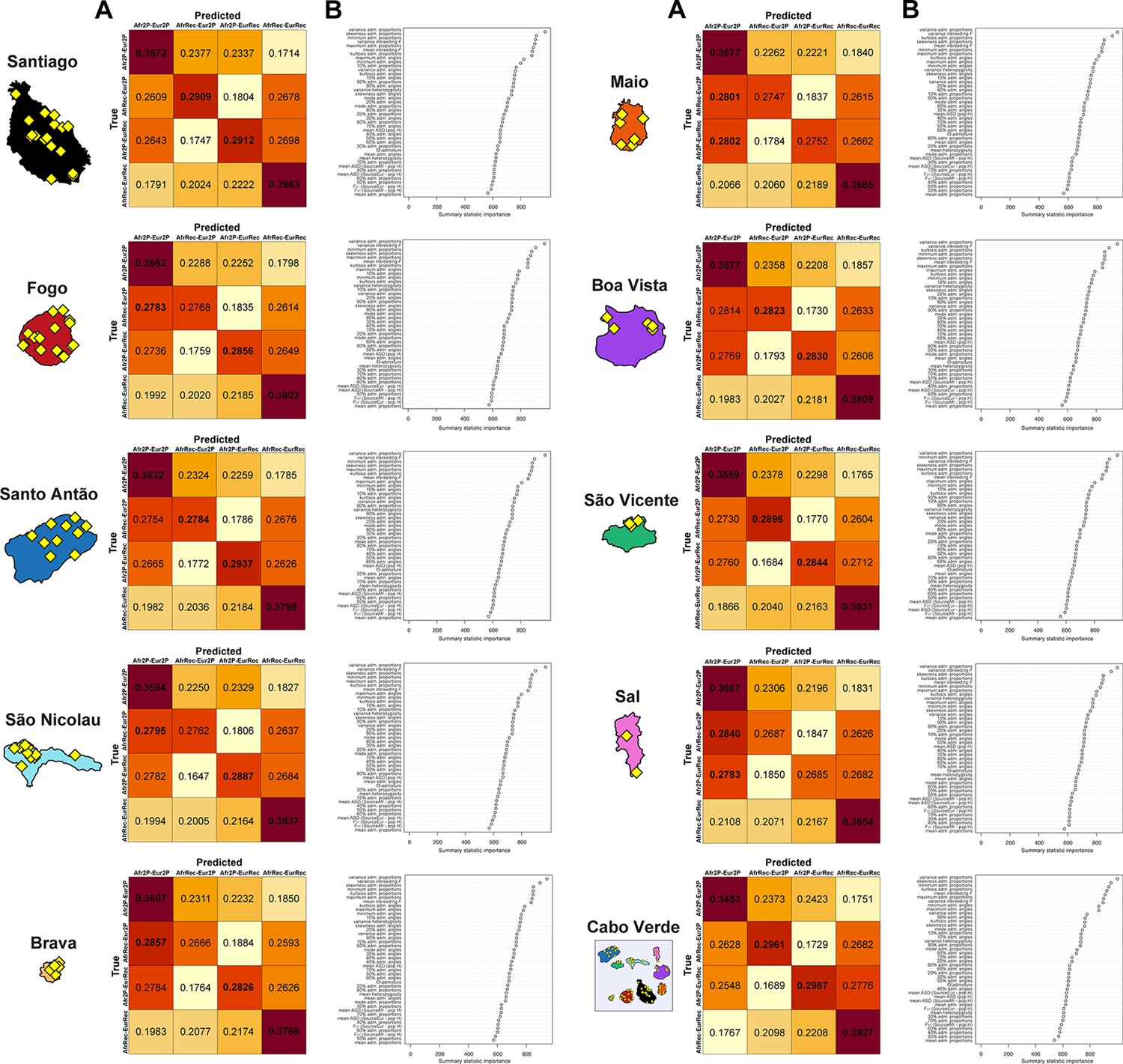
Random-Forest ABC scenario-choice cross validation results and summary-statistics’ importance.
We considered four competing scenarios as described in Genetic admixture histories in Cabo Verde inferred with MetHis-ABC and in Figure 6, with associated prior parameter distributions in Table 2 and 42 summary-statistics described in Table 3, for each Cabo Verdean birth-island and the 225 Cabo Verde-born individuals grouped in a single random mating population, separately. Cross-validation results are obtained by conducting RF scenario-choices using, in-turn, each 40,000 simulations (10,000 per competing scenario) as pseudo-observed data and the remaining 39,999 simulations as the reference table. We considered 1,000 trees in the random-forest for each analysis. Cross-validation results and associated summary-statistics’ importance for the RF decisions are obtained from the function abcrf in the R package abcrf.
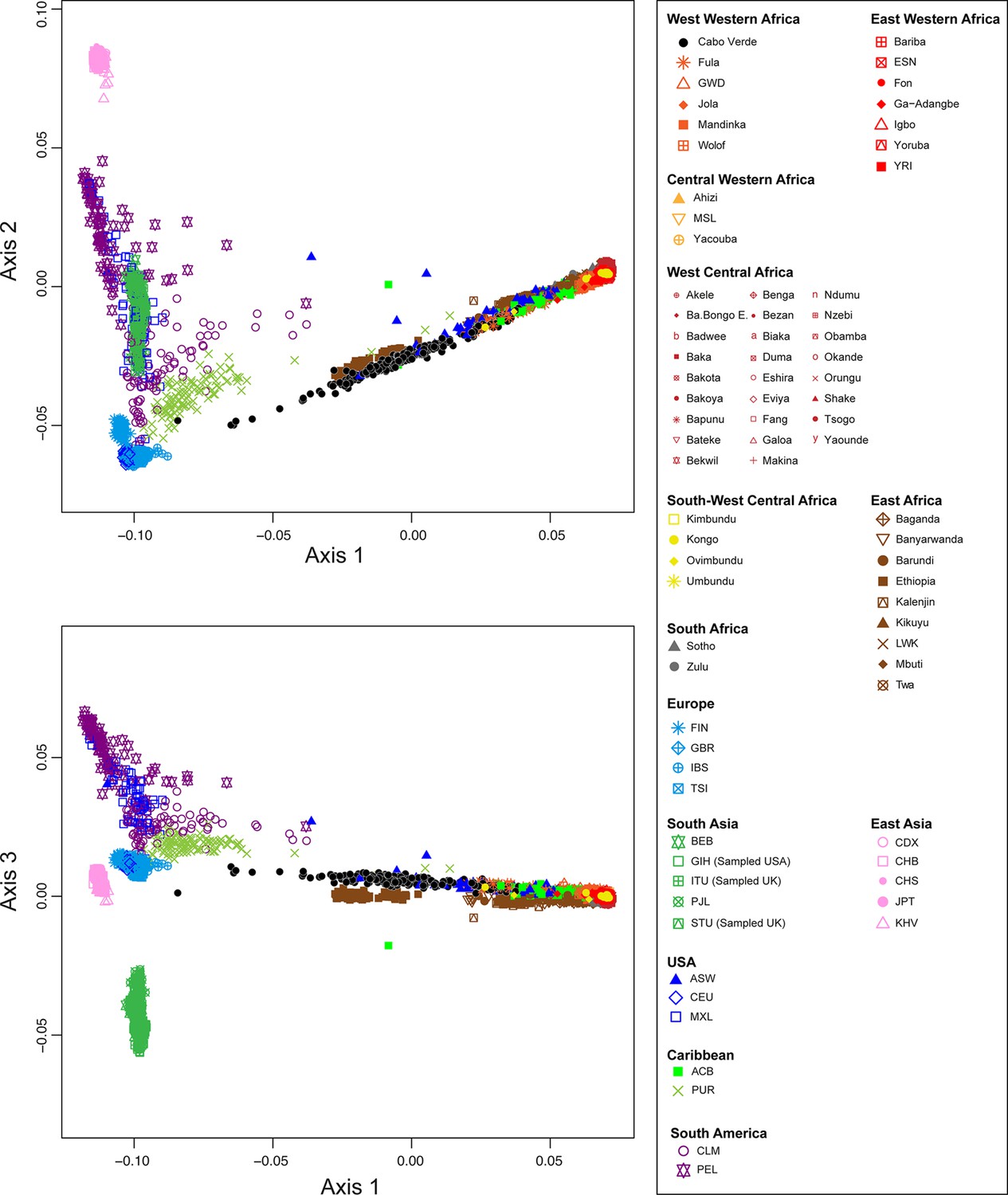
Appendix 2—figure 1 with 1 supplement
Multidimensional scaling three-dimensional projection of allele sharing pairwise dissimilarities, for all worldwide populations in our dataset.
Each individual in the plot is represented by a single point. See Figure 1—source data 1 for the population list used and Figure 1 for sample locations and symbols. (A) Axis 1 and 2; (B) Axis 1 and 3. 3D animated plot is provided in.gif format. We evaluate the Spearman correlation between 3D MDS projections and the original ASD pairwise matrix to evaluate the precision of the dimensionality reduction along the first three axes of the MDS. We find significant Spearman ρ of 0.9796 (p<2.2 × 10⁻¹⁶).
Appendix 2—figure 1—animation 1
3D animated MDS of pairwise allele sharing dissimilarities for all worldwide populations in our dataset.
Appendix 2—figure 2 with 1 supplement
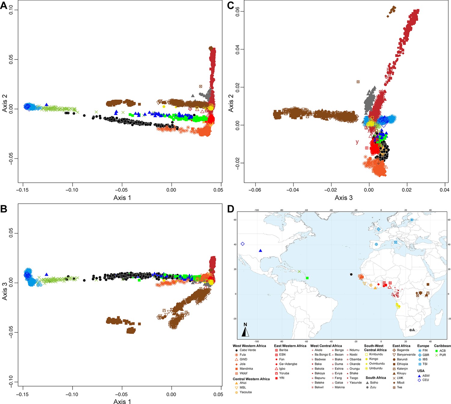
Multidimensional scaling three-dimensional projection of allele sharing pairwise dissimilarities, for all of the African, European and other admixed populations related to the TAST.
Each individual is represented by a single point. We removed all Asian and South American samples compared to the sample set employed in Appendix 2—figure 1, and recomputed the MDS based on this reduced sample set. See Figure 1—source data 1 for the population list used in these analyses. The sample map used in these analyses is extracted from Figure 1 and provided in panel D. (A) Axis 1 and 2; (B) Axis 2 and 3; (C) Axis 1 and 3. 3D animated plot is provided in.gif format. We evaluate the Spearman correlation between 3D MDS projections and the original ASD pairwise matrix to evaluate the precision of the dimensionality reduction along the first three axes of the MDS. We find Spearman ρ of 0.9392 (p<2.2 × 10⁻¹⁶).
Appendix 2—figure 2—animation 1
3D animated MDS of pairwise allele sharing dissimilarities for all of the African, European and other admixed populations related to the TAST.
Appendix 2—figure 3 with 1 supplement
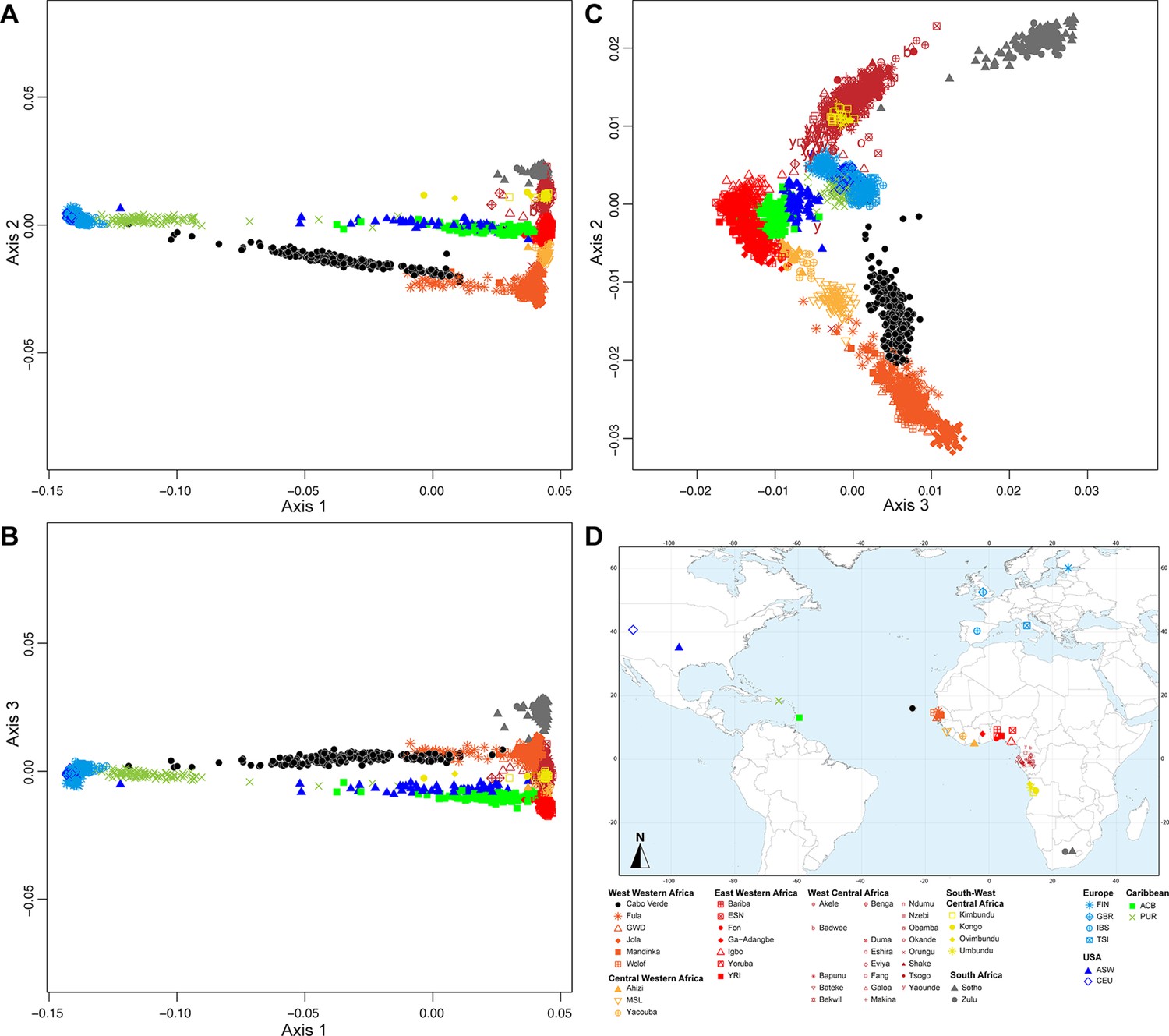
Multidimensional scaling three-dimensional projection of allele sharing pairwise dissimilarities, for a subset of African, European and other admixed populations related to the TAST.
Each individual is represented by a single point. We removed all East African and Central African hunter-gatherer samples (Baka, Bezan, Ba.Bongo, Ba.Koya, Ba.Twa, Bi.Aka, Mbuti) compared to the sample set employed in Appendix 2—figure 2, and recomputed the MDS based on this reduced sample set. See Figure 1—source data 1 for the population list used in these analyses. Sample map used in these analyses is extracted from Figure 1 and provided in panel D. (A) Axis 1 and 2; (B) Axis 2 and 3; (C) Axis 1 and 3. 3D animated plot is provided in.gif format. We evaluate the Spearman correlation between 3D MDS projections and the original ASD pairwise matrix to evaluate the precision of the dimensionality reduction along the first three axes of the MDS. We find Spearman ρ of 0.9450 (p<2.2 × 10⁻¹⁶).
Appendix 2—figure 3—animation 1
3D animated MDS of pairwise allele sharing dissimilarities for a subset of African, European and other admixed populations related to the TAST.
Appendix 2—figure 4 with 1 supplement
Multidimensional scaling three-dimensional projection of allele sharing pairwise dissimilarities, for the closest subsets of West African, European and other admixed populations related to the TAST.
Each individual is represented by a single point. We removed all West and South-West Central African samples, as well as South African samples, compared to the sample set employed in Appendix 2—figure 3, and recomputed the MDS based on this reduced sample set. See Figure 1—source data 1 for the population list used in these analyses. Sample map used in these analyses is extracted from Figure 1 and provided in panel D. (A) Axis 1 and 2; (B) Axis 2 and 3; (C) Axis 1 and 3. 3D animated plot is provided in.gif format. We evaluate the Spearman correlation between 3D MDS projections and the original ASD pairwise matrix to evaluate the precision of the dimensionality reduction along the first three axes of the MDS. We find Spearman ρ of 0.9636 (p<2.2 × 10⁻¹⁶).
Appendix 2—figure 4—animation 1
3D animated MDS of pairwise allele sharing dissimilarities for the closest subsets of West African, European and other admixed populations related to the TAST.
Appendix 3—figure 1
Alternative ADMIXTURE mode results for the individual genetic structure among Cabo Verdean, Barbadian-ACB and African-American ASW populations related to the TAST.
ADMIXTURE (Alexander et al., 2009) analyses using resampled individual sets for the population sets originally containing more than 50 individuals (Figure 1—source data 1). 225 unrelated Cabo Verdean-born individuals are grouped by island of birth (Figure 1—source data 1). All analyses considered 102,543 independent autosomal SNPs, for values of K between 2 and 15. 30 independent ADMIXTURE runs were performed for each value of K, and groups of runs (>2) providing similar results (all pairwise SSC >99.9%) were averaged in a single ‘mode’ result using CLUMPP (Jakobsson and Rosenberg, 2007), and plotted with DISTRUCT (Rosenberg, 2003). Number of runs in the presented modes are indicated below the value of K. All other modes are presented in Figure 3.
Appendix 4—figure 1
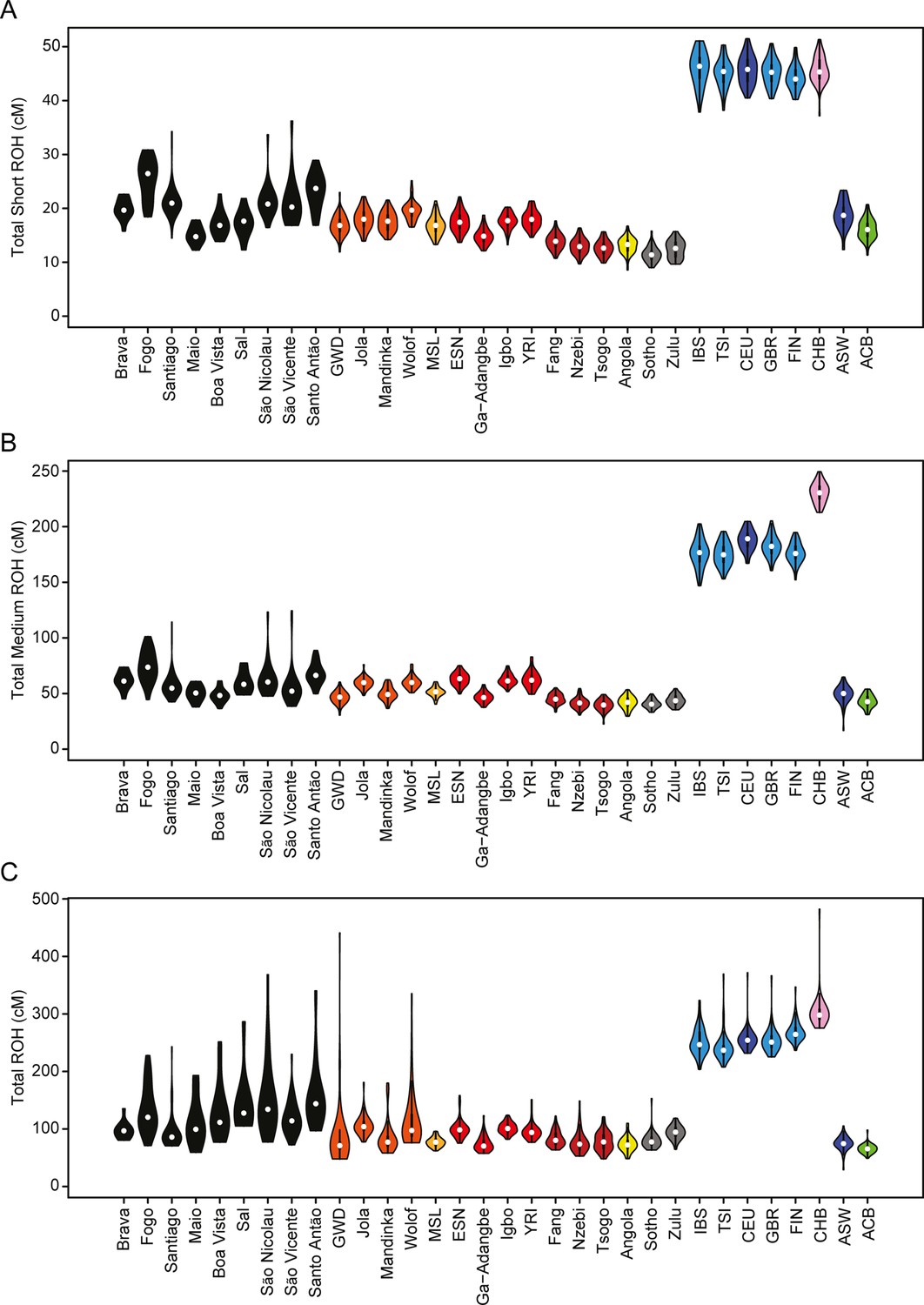
The distribution of (A) short, (B) medium, and (C) all ROH per individual, for each Cabo Verdean birth-island and other worldwide populations.
Appendix 4—figure 2
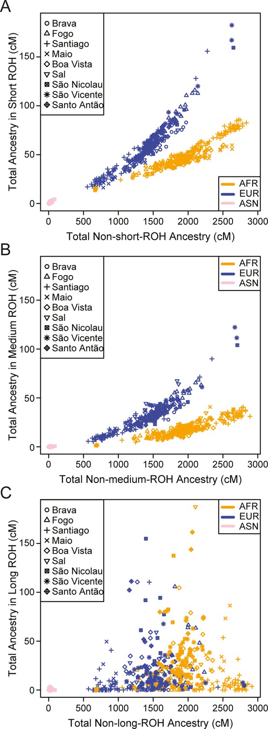
Individual total ancestry contained in (A) short, (B) medium, and (C) long ROH versus total ancestry not in that class ROH, for each Cabo Verdean birth-island and other worldwide populations.
Tables
Table 1
Mantel and partial-Mantel correlations between utterance frequency differences and covariables, and between genetic ASD and the same covariables, in 225 genetically unrelated Cabo Verde-born Kriolu-speaking individuals.
| Genetic ASD - 1,899,978 SNPs | Utterance-frequency Euclidean distances - 4831 uttered items | ||||||
|---|---|---|---|---|---|---|---|
| Mantel variable | Partial-Mantel control | n | Geographic scale | Spearman rho | 10,000 Mantel two-sided permutation p | Spearman rho | 10,000 Mantel two-sided permutation p |
| abs(Age difference) | -- | 225 | within and between islands | 0.1303 | <2.10–4 | 0.2215 | <2.10–4 |
| abs(Age difference) | log(Birth-loc. dist.) | 225 | within and between islands | 0.1348 | <2.10–4 | 0.2294 | <2.10–4 |
| log(Birth-loc. dist.) | -- | 225 | within and between islands | 0.2916 | <2.10–4 | 0.2794 | <2.10–4 |
| log(Birth-loc. dist.) | abs(Age difference) | 225 | within and between islands | 0.2935 | <2.10–4 | 0.2855 | <2.10–4 |
| abs(Education duration difference) | -- | 186 | within and between islands | 0.0168 | 0.2730 | 0.0962 | 0.0024 |
| abs(Education duration difference) | log(Birth-loc. dist.) | 186 | within and between islands | –0.0023 | 0.4900 | 0.0834 | 0.0071 |
| abs(Education duration difference) | -- | 185 | within and between islands | 0.0159 | 0.2825 | 0.1001 | 0.0014 |
| abs(Education duration difference) | log(Residence dist.) | 185 | within and between islands | –0.0041 | 0.4651 | 0.0824 | 0.0068 |
| log(Residence dist.) | -- | 224 | within and between islands | 0.1658 | <2.10–4 | 0.2145 | <2.10–4 |
| log(Residence dist.) | log(Birth-loc. dist.) | 224 | within and between islands | –0.0488 | 0.0005 | 0.0306 | 0.0682 |
| log(Birth-loc. dist.) | -- | 224 | within and between islands | 0.2889 | <2.10–4 | 0.2800 | <2.10–4 |
| log(Birth-loc. dist.) | log(Residence dist.) | 224 | within and between islands | 0.2445 | <2.10–4 | 0.1863 | <2.10–4 |
| log(Father Birth-loc. dist.) | -- | 222 | within and between islands | 0.2424 | <2.10–4 | 0.1704 | <2.10–4 |
| log(Father Birth-loc. dist.) | log(Birth-loc. dist.) | 222 | within and between islands | 0.0846 | 0.0014 | 0.0066 | 0.3915 |
| log(Mother Birth-loc. dist.) | -- | 224 | within and between islands | 0.2619 | <2.10–4 | 0.2634 | <2.10–4 |
| log(Mother Birth-loc. dist.) | log(Birth-loc. dist.) | 224 | within and between islands | 0.0748 | 0.0057 | 0.0853 | 0.0071 |
| abs(Age difference) | -- | 225 | within islands only | 0.2124 | 0.0006 | 0.2727 | <2.10–4 |
| abs(Age difference) | log(Birth-loc. dist.) | 225 | within islands only | 0.1648 | 0.0041 | 0.2546 | <2.10–4 |
| log(Birth-loc. dist.) | -- | 225 | within islands only | 0.3460 | <2.10–4 | 0.1412 | 0.0401 |
| log(Birth-loc. dist.) | abs(Age difference) | 225 | within islands only | 0.3212 | <2.10–4 | 0.0990 | 0.1030 |
| abs(Education duration difference) | -- | 186 | within islands only | –0.0370 | 0.3077 | 0.1287 | 0.0440 |
| abs(Education duration difference) | log(Birth-loc. dist.) | 186 | within islands only | –0.0537 | 0.2330 | 0.1239 | 0.0496 |
| abs(Education duration difference) | -- | 185 | within islands only | –0.0382 | 0.3037 | 0.1421 | 0.0292 |
| abs(Education duration difference) | log(Residence dist.) | 185 | within islands only | –0.0491 | 0.2566 | 0.1202 | 0.0546 |
| log(Residence dist.) | -- | 224 | within islands only | –0.0667 | 0.1907 | 0.0982 | 0.0911 |
| log(Residence dist.) | log(Birth-loc. dist.) | 224 | within islands only | –0.0549 | 0.2319 | 0.1063 | 0.0704 |
| log(Birth-loc. dist.) | -- | 224 | within islands only | 0.3465 | <2.10–4 | 0.1537 | 0.0282 |
| log(Birth-loc. dist.) | log(Residence dist.) | 224 | within islands only | 0.3446 | <2.10–4 | 0.1589 | 0.0230 |
| log(Father Birth-loc. dist.) | -- | 222 | within islands only | 0.2660 | 0.0006 | 0.0160 | 0.4123 |
| log(Father Birth-loc. dist.) | log(Birth-loc. dist.) | 222 | within islands only | 0.2187 | 0.0045 | –0.0111 | 0.4546 |
| log(Mother Birth-loc. dist.) | -- | 224 | within islands only | 0.2240 | 0.0034 | 0.1283 | 0.0423 |
| log(Mother Birth-loc. dist.) | log(Birth-loc. dist.) | 224 | within islands only | 0.1563 | 0.0303 | 0.1000 | 0.0925 |
-
Table 1—source data 1
Mantel correlations among individual birth-places, residence-places, maternal and paternal birth places, age, and academic education duration.
- https://cdn.elifesciences.org/articles/79827/elife-79827-table1-data1-v3.xlsx
Table 2
Prior distributions for the parameters of four competing scenarios for the admixture history of Cabo Verde islands.
Parameters are presented in Figure 6 and described in Material and Methods.
| Description | Scenario | Model parameter | Prior | Conditions |
|---|---|---|---|---|
| African admixture-pulse times | 1, 2 | tAfr,p1 | Uniform [1 , 20] in discrete generations, a range corresponding to between ~1485 and~1960 in years CE | tAfr,p1 >tAfr,p2 |
| tAfr,p2 | ||||
| European admixture-pulse times | 1, 3 | tEur,p1 | Uniform [1 , 20] in discrete generations, a range corresponding to between ~1485 and~1960 in years CE | tEur,p1 >tEur,p2 |
| tEur,p2 | ||||
| African admixture period start and end times | 2, 4 | tAfr,t1 | Uniform [1 , 20] in discrete generations, a range corresponding to between ~1485 and~1960 in years CE | tAfr,t1 >tAfr,t2 |
| tAfr,t2 | ||||
| European admixture period start and end times | 3, 4 | tEur,t1 | Uniform [1 , 20] in discrete generations, a range corresponding to between ~1485 and~1960 in years CE | tEur,t1 >tEur,t2 |
| tEur,t2 | ||||
| African admixture-pulse intensities | 1, 2 | sAfr,tAfr,p1 | Uniform [0, 1] | sAfr,g + sEur,g = 1 – hg, with hg in [0,1] |
| sAfr,tAfr,p2 | ||||
| European admixture-pulse intensities | 1, 3 | sEur,tEur,p1 | Uniform [0, 1] | |
| sEur,tEur,p2 | ||||
| African admixture period intensity parameters | 2, 4 | sAfr,tAfr,t1 | Uniform [0, 1] | sAfr,tAfr,t1 ≥sAfr,tAfr,t2 |
| sAfr,tAfr,t2 | Uniform [0, 1] | sAfr,g + sEur,g = 1 – hg, with hg in [0,1] | ||
| uAfr | Uniform [0, 0.5] | |||
| European admixture period intensity parameters | 3, 4 | sEur,tEur,t1 | Uniform [0, 1] | sEur,tEur,t1 ≥sEur,tEur,t2 |
| sEur,tEur,t2 | Uniform [0, 1] | sAfr,g + sEur,g = 1 – hg, with hg in [0,1] | ||
| uEur | Uniform [0, 0.5] | |||
| Admixture pulse at the foundation | 1, 2, 3, 4 | sAfr,0 | Uniform [0, 1] | sEur,0 = 1 – sAfr,0 |
| Founding reproductive population size | 1, 2, 3, 4 | N0 | Uniform [10, 1000] | N0 ≤ N20 |
| Current reproductive population size | 1, 2, 3, 4 | N20 | Uniform [100, 100,000] | |
| Steepness of the reproductive population size increase | 1, 2, 3, 4 | uN | Uniform [0, 0.5] | |
Table 3
Summary-statistics used for MetHis-machine-learning ABC inferences.
All 42 statistics were computed using the summary-statistics computation tool embedded in MetHis (Fortes‐Lima et al., 2021).
| Summary Statistics for ABC inference | Nunber of statistics | Reference | |
|---|---|---|---|
| within population | Mean ASD within population H | 1 | Bowcock et al., 1994 |
| Mean Heterozygosity (SNP by SNP) within population H | 1 | Nei, 1978 | |
| Variance Heterozygosity (SNP by SNP) within population H | 1 | Nei, 1978 | |
| Mean inbreeding F within population H | 1 | Danecek et al., 2011 | |
| Variance inbreeding F within population H | 1 | Danecek et al., 2011 | |
| admixture pattern | Mode ASD-MDS African admixture proportions in population H | 1 | Fortes‐Lima et al., 2021; Verdu and Rosenberg, 2011 |
| Mean ASD-MDS African admixture proportions in population H | 1 | Fortes‐Lima et al., 2021; Verdu and Rosenberg, 2011 | |
| Variance ASD-MDS African admixture proportions in population H | 1 | Fortes‐Lima et al., 2021; Verdu and Rosenberg, 2011 | |
| Skewness ASD-MDS African admixture proportions in population H | 1 | Fortes‐Lima et al., 2021; Verdu and Rosenberg, 2011 | |
| Kurtosis ASD-MDS African admixture proportions in population H | 1 | Fortes‐Lima et al., 2021; Verdu and Rosenberg, 2011 | |
| Min ASD-MDS African admixture proportions in population H | 1 | Fortes‐Lima et al., 2021; Verdu and Rosenberg, 2011 | |
| Max ASD-MDS African admixture proportions in population H | 1 | Fortes‐Lima et al., 2021; Verdu and Rosenberg, 2011 | |
| Deciles of ASD-MDS African admixture proportions in population H | 9 | Fortes‐Lima et al., 2021; Verdu and Rosenberg, 2011 | |
| Mode ASD-MDS ‘African-European angles’ in population H | 1 | This study; Appendix 1—figure 2 | |
| Mean ASD-MDS ‘African-European angles’ in population H | 1 | This study; Appendix 1—figure 2 | |
| Variance ASD-MDS ‘African-European angles’ in population H | 1 | This study; Appendix 1—figure 2 | |
| Skewness ASD-MDS ‘African-European angles’ in population H | 1 | This study; Appendix 1—figure 2 | |
| Kurtosis ASD-MDS ‘African-European angles’ in population H | 1 | This study; Appendix 1—figure 2 | |
| Min ASD-MDS ‘African-European angles’ in population H | 1 | This study; Appendix 1—figure 2 | |
| Max ASD-MDS ‘African-European angles’ in population H | 1 | This study; Appendix 1—figure 2 | |
| Deciles of ASD-MDS ‘African-European angles’ in population H | 9 | This study; Appendix 1—figure 2 | |
| between populations | Fst (African Source - Population H) | 1 | Weir and Cockerham, 1984 |
| Fst (European Source - Population H) | 1 | Weir and Cockerham, 1984 | |
| Mean ASD (African Source - Population H) | 1 | Bowcock et al., 1994 | |
| Mean ASD (European Source - Population H) | 1 | Bowcock et al., 1994 | |
| f3 (Population H; European Source, African Source) | 1 | Patterson et al., 2012 | |
Appendix 1—table 1
Average parameter posterior random cross-validation error across all model parameters as a function of the number of neurons in the hidden layer and the rejection tolerance level (number of simulations retained for training the Neural-Network) under the winning scenario for each island respectively.
For each island separately, and for the 225 Cabo Verde-born individuals grouped as a single “Cabo Verde” population, we considered, 1,000 random simulations in-turn as pseudo-observed data to estimate posterior parameter distributions and 100,000 total simulations in the reference table. For each cross-validation procedure, we considered between 5 and 11 neurons in the hidden layer (“NN-HL”) for the winning scenarios with 12 original parameters, and between 5 and 12 NN-HL for the winning scenarios with 13 original parameters. We considered three different tolerance levels of 0.01, 0.03, and 0.1 (“Tol.”) corresponding, respectively, to 1,000, 3,000, and 10,000 simulations, in turn closest to each one of the 1,000 cross-validation pseudo-observed simulation retained for training the NN. The median values of posterior parameter distributions were used as point estimates for the calculation of the error of each parameter (Csilléry et al., 2012). For each birth-island and Cabo Verde as a whole, and corresponding winning scenario, separately, we considered, for further posterior parameter estimation using the observed “real” data, only the pair of tolerance level and number of hidden neurons that minimized the average error on posterior parameter estimations across all parameters (indicated in bold in the table).
| Individual birth-island | SANTIAGO | FOGO | SANTO ANTAO | SAO NICOLAU | BRAVA | MAIO | BOA VISTA | SAO VICENTE | SAL | CABO VERDE | |
|---|---|---|---|---|---|---|---|---|---|---|---|
| Winning scenario | Scenario 1: Afr2pulses-Eur2pulses | Scenario 1: Afr2pulses-Eur2pulses | Scenario 1: Afr2pulses-Eur2pulses | Scenario 1: Afr2pulses-Eur2pulses | Scenario 1: Afr2pulses-Eur2pulses | Scenario 1: Afr2pulses-Eur2pulses | Scenario 2: Afr2pulses-EurReccurring | Scenario 3: AfrReccurring-Eur2pulses | Scenario 2: Afr2pulses-EurReccurring | Scenario 1: Afr2pulses-Eur2pulses | |
| Number of scenario parameters | 12 | 12 | 12 | 12 | 12 | 12 | 13 | 13 | 13 | 12 | |
| NN-HL=5 | Tol.=0.01 | 0.79264 | 0.79943 | 0.80170 | 0.79380 | 0.81251 | 0.83232 | 0.79972 | 0.77795 | 0.82888 | 0.79532 |
| NN-HL=5 | Tol.=0.03 | 0.80866 | 0.81252 | 0.81257 | 0.80711 | 0.81703 | 0.83470 | 0.79708 | 0.80208 | 0.81783 | 0.83438 |
| NN-HL=5 | Tol.=0.1 | 0.84002 | 0.84001 | 0.84662 | 0.84970 | 0.84526 | 0.85366 | 0.83374 | 0.82312 | 0.83264 | 0.85271 |
| NN-HL=6 | Tol.=0.01 | 0.77139 | 0.80186 | 0.79800 | 0.80765 | 0.81085 | 0.82516 | 0.78239 | 0.77743 | 0.81601 | 0.82118 |
| NN-HL=6 | Tol.=0.03 | 0.79501 | 0.81397 | 0.80533 | 0.80483 | 0.83318 | 0.83673 | 0.80492 | 0.80127 | 0.81325 | 0.82982 |
| NN-HL=6 | Tol.=0.1 | 0.84684 | 0.84072 | 0.84028 | 0.84484 | 0.85753 | 0.85428 | 0.82136 | 0.81617 | 0.83773 | 0.84745 |
| NN-HL=7 | Tol.=0.01 | 0.78525 | 0.79836 | 0.79075 | 0.81595 | 0.82657 | 0.82662 | 0.79304 | 0.77898 | 0.80415 | 0.80413 |
| NN-HL=7 | Tol.=0.03 | 0.80899 | 0.81151 | 0.81000 | 0.81035 | 0.83069 | 0.83474 | 0.80060 | 0.79491 | 0.81855 | 0.83622 |
| NN-HL=7 | Tol.=0.1 | 0.85600 | 0.84844 | 0.83704 | 0.84737 | 0.85071 | 0.85582 | 0.81083 | 0.81619 | 0.83779 | 0.85601 |
| NN-HL=8 | Tol.=0.01 | 0.78512 | 0.79805 | 0.79127 | 0.80886 | 0.82241 | 0.83397 | 0.77998 | 0.78077 | 0.80992 | 0.80783 |
| NN-HL=8 | Tol.=0.03 | 0.80595 | 0.81077 | 0.81353 | 0.82455 | 0.82334 | 0.83718 | 0.79490 | 0.78639 | 0.80666 | 0.83396 |
| NN-HL=8 | Tol.=0.1 | 0.83938 | 0.84904 | 0.83681 | 0.85231 | 0.84982 | 0.84614 | 0.83499 | 0.81671 | 0.82696 | 0.84774 |
| NN-HL=9 | Tol.=0.01 | 0.77910 | 0.79899 | 0.81027 | 0.80103 | 0.81898 | 0.82483 | 0.79744 | 0.78619 | 0.81770 | 0.80542 |
| NN-HL=9 | Tol.=0.03 | 0.81192 | 0.81046 | 0.81474 | 0.81642 | 0.82593 | 0.82631 | 0.80830 | 0.78640 | 0.82212 | 0.84165 |
| NN-HL=9 | Tol.=0.1 | 0.84379 | 0.84721 | 0.83676 | 0.84813 | 0.85218 | 0.85223 | 0.83254 | 0.81696 | 0.81723 | 0.85381 |
| NN-HL=10 | Tol.=0.01 | 0.78593 | 0.79615 | 0.80275 | 0.79444 | 0.80692 | 0.82095 | 0.80121 | 0.77644 | 0.81801 | 0.80485 |
| NN-HL=10 | Tol.=0.03 | 0.80159 | 0.80818 | 0.81143 | 0.80949 | 0.82496 | 0.82787 | 0.79994 | 0.78673 | 0.81565 | 0.82157 |
| NN-HL=10 | Tol.=0.1 | 0.85245 | 0.84242 | 0.84222 | 0.83444 | 0.85410 | 0.85424 | 0.83049 | 0.81742 | 0.84950 | 0.84183 |
| NN-HL=11 | Tol.=0.01 | 0.79994 | 0.81073 | 0.78479 | 0.78709 | 0.82527 | 0.84091 | 0.79414 | 0.77365 | 0.79984 | 0.80239 |
| NN-HL=11 | Tol.=0.03 | 0.82611 | 0.80802 | 0.80825 | 0.81653 | 0.82511 | 0.82334 | 0.80234 | 0.80333 | 0.81750 | 0.82959 |
| NN-HL=11 | Tol.=0.1 | 0.84914 | 0.83930 | 0.84011 | 0.84941 | 0.85471 | 0.85756 | 0.82120 | 0.81919 | 0.83044 | 0.85282 |
| NN-HL=12 | Tol.=0.01 | na | na | na | na | na | na | 0.79915 | 0.78138 | 0.81418 | na |
| NN-HL=12 | Tol.=0.03 | na | na | na | na | na | na | 0.79959 | 0.79306 | 0.81551 | na |
| NN-HL=12 | Tol.=0.1 | na | na | na | na | na | na | 0.81731 | 0.82090 | 0.82284 | na |
Appendix 5—table 1
SantiagoNN-ABC posterior parameter estimations for Santiago island, cross-validation posterior parameter errors, and cross-validation 95% Credibility Interval accuracies.
Cross-validation errors and 95% CI accuracies are based on 1000 NN-ABC posterior parameter inferences using, in turn, each one of the 1000 simulations closest to the observed data used as pseudo-observed data, and the remaining 99,999 simulations as the reference table. Error calculations are based on the mode and, separately, the median point estimate for each 1000 pseudo-observed simulations posterior parameter estimation, compared to the known parameter used for simulation. We considered six neurons in the hidden layer and a tolerance level of 0.01 (1000 simulations) for all posterior parameter estimation in this analysis as identified in Appendix 1—table 1. Plotted distributions for posterior parameter estimations can be found in Figure 7—figure supplements 1–3.
| SANTIAGO | Parameter posterior estimation | 1,000 cross-validation errors | |||||
|---|---|---|---|---|---|---|---|
| Afr2P-Eur2P scenario parameters | Mode | Median | 50% Credibility Interval | 95% Credibility Interval | Mode mean absolute error | Median mean absolute error | 95% CI length accuracy |
| Ne.0 | 142 | 431 | [194 - 692] | [28 - 974] | 305 | 255 | 0.059 |
| Ne.20 | 92109 | 80077 | [63220–91349] | [30408–98975] | 25426 | 21558 | 0.045 |
| u.Ne | 0.440 | 0.365 | [0.284–0.438] | [0.150–0.494] | 0.113 | 0.096 | 0.042 |
| sAfr,0 | 0.8816 | 0.6365 | [0.3884–0.8415] | [0.0538–0.9858] | 0.3147 | 0.2507 | 0.056 |
| tAfr,p1 | 13.9 | 9.2 | [4.9–13.4] | [1.7–16.8] | 5.3 | 4.2 | 0.101 |
| sAfr,tAfr,p1 | 0.7844 | 0.5986 | [0.3421–0.7861] | [0.0420–0.9479] | 0.2618 | 0.2204 | 0.054 |
| tAfr,p2 | 17.2 | 16.6 | [15.2–17.5] | [10.0–18.9] | 1.8 | 1.6 | 0.199 |
| sAfr,tAfr,p2 | 0.6837 | 0.5913 | [0.3894–0.7241] | [0.0642–0.9038] | 0.1597 | 0.1458 | 0.052 |
| tEur,p1 | 3.4 | 7.5 | [4.3–11.1] | [2.3–15.9] | 4.0 | 3.1 | 0.161 |
| sEur,tEur,p1 | 0.1617 | 0.3969 | [0.1957–0.6606] | [0.0185–0.9564] | 0.3042 | 0.2439 | 0.056 |
| tEur,p2 | 19.1 | 18.7 | [17.7–19.2] | [11.7–19.6] | 3.0 | 2.9 | 0.115 |
| sEur,tEur,p2 | 0.0258 | 0.0684 | [0.0250–0.1501] | [0.0028–0.6021] | 0.2749 | 0.2254 | 0.057 |
Appendix 5—table 2
Fogo NN-ABC posterior parameter estimations for Fogo island, cross-validation posterior parameter errors, and cross-validation 95% Credibility Interval accuracies.
Cross-validation errors and 95% CI accuracies are based on 1000 NN-ABC posterior parameter inferences using, in turn, each one of the 1000 simulations closest to the observed data used as pseudo-observed data, and the remaining 99,999 simulations as the reference table. Error calculations are based on the mode and, separately, the median point estimate for each 1000 pseudo-observed simulations posterior parameter estimation, compared to the known parameter used for simulation. We considered 10 neurons in the hidden layer and a tolerance level of 0.01 (1000 simulations) for all posterior parameter estimation in this analysis as identified in Appendix 1—table 1. Plotted distributions for posterior parameter estimations can be found in Figure 7—figure supplements 1–3.
| FOGO | Parameter posterior estimation | 1000 cross-validation errors | |||||
|---|---|---|---|---|---|---|---|
| Afr2P-Eur2P scenario parameters | Mode | Median | 50% Credibility Interval | 95% Credibility Interval | Mode mean absolute error | Median mean absolute error | 95% CI length accuracy |
| Ne.0 | 349 | 511 | [274 - 737] | [44 - 969] | 295 | 253 | 0.063 |
| Ne.20 | 90370 | 72023 | [50948–87248] | [18011–98846] | 27142 | 22749 | 0.057 |
| u.Ne | 0.115 | 0.150 | [0.104–0.230] | [0.055–0.447] | 0.085 | 0.081 | 0.074 |
| sAfr,0 | 0.7407 | 0.6831 | [0.5218–0.8152] | [0.1679–0.9600] | 0.2936 | 0.2432 | 0.069 |
| tAfr,p1 | 13.3 | 12.0 | [8.1–14.4] | [4.7–16.9] | 4.2 | 3.3 | 0.157 |
| sAfr,tAfr,p1 | 0.4667 | 0.4549 | [0.2286–0.6721] | [0.0251–0.9555] | 0.2498 | 0.2315 | 0.056 |
| tAfr,p2 | 19.5 | 19.3 | [18.9–19.5] | [15.6–19.8] | 2.6 | 2.5 | 0.100 |
| sAfr,tAfr,p2 | 0.1174 | 0.2034 | [0.1051–0.3560] | [0.0120–0.8225] | 0.2032 | 0.1891 | 0.060 |
| tEur,p1 | 2.5 | 5.3 | [2.7–8.8] | [1.9–13.9] | 3.6 | 3.0 | 0.216 |
| sEur,tEur,p1 | 0.1149 | 0.2234 | [0.1146–0.3943] | [0.0223–0.8383] | 0.2804 | 0.2371 | 0.062 |
| tEur,p2 | 16.7 | 15.5 | [13.1–16.8] | [6.7–18.2] | 3.2 | 3.0 | 0.070 |
| sEur,tEur,p2 | 0.2101 | 0.2428 | [0.1393–0.3966] | [0.0157–0.8485] | 0.1751 | 0.1686 | 0.060 |
Appendix 5—table 3
Santo AntãoNN-ABC posterior parameter estimations for Santo Antão island, cross-validation posterior parameter errors, and cross-validation 95% Credibility Interval accuracies.
Cross-validation errors and 95% CI accuracies are based on 1000 NN-ABC posterior parameter inferences using, in turn, each one of the 1000 simulations closest to the observed data used as pseudo-observed data, and the remaining 99,999 simulations as the reference table. Error calculations are based on the mode and, separately, the median point estimate for each 1000 pseudo-observed simulations posterior parameter estimation, compared to the known parameter used for simulation. We considered 11 neurons in the hidden layer and a tolerance level of 0.01 (1000 simulations) for all posterior parameter estimation in this analysis as identified in Appendix 1—table 1. Plotted distributions for posterior parameter estimations can be found in Figure 7—figure supplements 1–3.
| SANTO ANTAO | Parameter posterior estimation | 1,000 cross-validation errors | |||||
|---|---|---|---|---|---|---|---|
| Afr2P-Eur2P scenario parameters | Mode | Median | 50% Credibility Interval | 95% Credibility Interval | Mode mean absolute error | Median mean absolute error | 95% CI length accuracy |
| Ne.0 | 411 | 469 | [254 - 706] | [26 - 964] | 254 | 228 | 0.071 |
| Ne.20 | 12056 | 41256 | [17145–69559] | [3570–96855] | 32106 | 25308 | 0.051 |
| u.Ne | 0.035 | 0.053 | [0.033–0.093] | [0.015–0.334] | 0.072 | 0.067 | 0.056 |
| sAfr,0 | 0.8047 | 0.5681 | [0.2995–0.7964] | [0.0260–0.9839] | 0.3029 | 0.2586 | 0.068 |
| tAfr,p1 | 2.4 | 4.9 | [2.9–7.4] | [1.9–11.9] | 3.3 | 2.6 | 0.164 |
| sAfr,tAfr,p1 | 0.7574 | 0.6255 | [0.3644–0.7916] | [0.0451–0.9749] | 0.2512 | 0.2283 | 0.055 |
| tAfr,p2 | 13.6 | 11.6 | [7.7–14.9] | [3.0–18.5] | 2.8 | 2.7 | 0.072 |
| sAfr,tAfr,p2 | 0.6294 | 0.4716 | [0.2596–0.6733] | [0.0338–0.9233] | 0.2435 | 0.2150 | 0.049 |
| tEur,p1 | 3.2 | 5.8 | [3.2–10.2] | [2.6–15.6] | 2.6 | 2.4 | 0.265 |
| sEur,tEur,p1 | 0.1542 | 0.3592 | [0.1709–0.6051] | [0.0216–0.9522] | 0.2767 | 0.2347 | 0.059 |
| tEur,p2 | 18.1 | 17.2 | [14.8–18.2] | [7.6–19.1] | 3.2 | 3.0 | 0.074 |
| sEur,tEur,p2 | 0.0467 | 0.0847 | [0.0416–0.1656] | [0.0056–0.6382] | 0.1868 | 0.1763 | 0.059 |
Appendix 5—table 4
São NicolauNN-ABC posterior parameter estimations for São Nicolau island, cross-validation posterior parameter errors, and cross-validation 95% Credibility Interval accuracies.
Cross-validation errors and 95% CI accuracies are based on 1000 NN-ABC posterior parameter inferences using, in turn, each one of the 1000 simulations closest to the observed data used as pseudo-observed data, and the remaining 99,999 simulations as the reference table. Error calculations are based on the mode and, separately, the median point estimate for each 1000 pseudo-observed simulations posterior parameter estimation, compared to the known parameter used for simulation. We considered 11 neurons in the hidden layer and a tolerance level of 0.01 (1000 simulations) for all posterior parameter estimation in this analysis as identified in Appendix 1—table 1. Plotted distributions for posterior parameter estimations can be found in Figure 7—figure supplements 1–3.
| SAO NICOLAU | Parameter posterior estimation | 1000 cross-validation errors | |||||
|---|---|---|---|---|---|---|---|
| Afr2P-Eur2P scenario parameters | Mode | Median | 50% Credibility Interval | 95% Credibility Interval | Mode mean absolute error | Median mean absolute error | 95% CI length accuracy |
| Ne.0 | 360 | 457 | [238 - 734] | [34 - 979] | 309 | 255 | 0.059 |
| Ne.20 | 28767 | 48793 | [25155–70475] | [3686–96753] | 27,502 | 23,452 | 0.055 |
| u.Ne | 0.135 | 0.238 | [0.133–0.358] | [0.025–0.483] | 0.132 | 0.113 | 0.057 |
| sAfr,0 | 0.3249 | 0.4730 | [0.2491–0.7393] | [0.0327–0.9752] | 0.3017 | 0.2461 | 0.051 |
| tAfr,p1 | 2.4 | 5.2 | [2.7–9.5] | [1.3–15.5] | 5.9 | 4.5 | 0.145 |
| sAfr,tAfr,p1 | 0.1695 | 0.3133 | [0.1584–0.5404] | [0.0171–0.9262] | 0.2897 | 0.2363 | 0.069 |
| tAfr,p2 | 14.6 | 14.5 | [13.2–14.9] | [8.3–16.4] | 1.5 | 1.4 | 0.522 |
| sAfr,tAfr,p2 | 0.7132 | 0.6398 | [0.4900–0.7736] | [0.0877–0.9380] | 0.1044 | 0.0981 | 0.055 |
| tEur,p1 | 2.7 | 6.7 | [3.5–10.8] | [2.0–16.1] | 4.6 | 3.5 | 0.139 |
| sEur,tEur,p1 | 0.1193 | 0.3240 | [0.1547–0.5711] | [0.0145–0.9460] | 0.2806 | 0.2394 | 0.048 |
| tEur,p2 | 19.2 | 19.0 | [17.7–19.4] | [10.3–19.8] | 3.3 | 2.9 | 0.199 |
| sEur,tEur,p2 | 0.0297 | 0.0731 | [0.0295–0.1465] | [0.0038–0.6642] | 0.2419 | 0.2067 | 0.065 |
Appendix 5—table 5
Brava NN-ABC posterior parameter estimations for Brava island, cross-validation posterior parameter errors, and cross-validation 95% Credibility Interval accuracies.
Cross-validation errors and 95% CI accuracies are based on 1000 NN-ABC posterior parameter inferences using, in turn, each one of the 1000 simulations closest to the observed data used as pseudo-observed data, and the remaining 99,999 simulations as the reference table. Error calculations are based on the mode and, separately, the median point estimate for each 1000 pseudo-observed simulations posterior parameter estimation, compared to the known parameter used for simulation. We considered 10 neurons in the hidden layer and a tolerance level of 0.01 (1000 simulations) for all posterior parameter estimation in this analysis as identified in Appendix 1—table 1. Plotted distributions for posterior parameter estimations can be found in Figure 7—figure supplements 1–3.
| BRAVA | Parameter posterior estimation | 1000 cross-validation errors | |||||
|---|---|---|---|---|---|---|---|
| Afr2P-Eur2P scenario parameters | Mode | Median | 50% Credibility Interval | 95% Credibility Interval | Mode mean absolute error | Median mean absolute error | 95% CI length accuracy |
| Ne.0 | 495 | 501 | [309 - 696] | [63 - 919] | 308 | 254 | 0.068 |
| Ne.20 | 3278 | 7337 | [2908–17935] | [647–73114] | 31523 | 24989 | 0.056 |
| u.Ne | 0.435 | 0.420 | [0.374–0.455] | [0.243–0.494] | 0.077 | 0.073 | 0.050 |
| sAfr,0 | 0.7337 | 0.5666 | [0.3452–0.7698] | [0.0497–0.9737] | 0.2836 | 0.2405 | 0.059 |
| tAfr,p1 | 1.6 | 2.8 | [1.5–5.3] | [1.1–12.2] | 3.9 | 3.1 | 0.159 |
| sAfr,tAfr,p1 | 0.7403 | 0.6688 | [0.4987–0.7995] | [0.1353–0.9685] | 0.2418 | 0.2232 | 0.060 |
| tAfr,p2 | 15.7 | 13.6 | [8.4–16.3] | [2.4–19.2] | 2.8 | 2.7 | 0.069 |
| sAfr,tAfr,p2 | 0.1261 | 0.2473 | [0.1272–0.3647] | [0.0191–0.8266] | 0.2118 | 0.1905 | 0.058 |
| tEur,p1 | 3.6 | 7.3 | [4.1–11.1] | [2.8–16.1] | 3.4 | 2.9 | 0.204 |
| sEur,tEur,p1 | 0.0157 | 0.0352 | [0.0116–0.1161] | [0.0007–0.7239] | 0.2658 | 0.2338 | 0.064 |
| tEur,p2 | 17.9 | 16.3 | [12.5–18.0] | [4.2–19.3] | 3.3 | 3.1 | 0.054 |
| sEur,tEur,p2 | 0.1281 | 0.1697 | [0.1054–0.2554] | [0.0188–0.6504] | 0.1844 | 0.1716 | 0.057 |
Appendix 5—table 6
MaioNN-ABC posterior parameter estimations for Maio island, cross-validation posterior parameter errors, and cross-validation 95% Credibility Interval accuracies.
Cross-validation errors and 95% CI accuracies are based on 1000 NN-ABC posterior parameter inferences using, in turn, each one of the 1000 simulations closest to the observed data used as pseudo-observed data, and the remaining 99,999 simulations as the reference table. Error calculations are based on the mode and, separately, the median point estimate for each 1000 pseudo-observed simulations posterior parameter estimation, compared to the known parameter used for simulation. We considered 10 neurons in the hidden layer and a tolerance level of 0.01 (1000 simulations) for all posterior parameter estimation in this analysis as identified in Appendix 1—table 1. Plotted distributions for posterior parameter estimations can be found in Figure 7—figure supplements 1–3.
| MAIO | Parameter posterior estimation | 1000 cross-validation errors | |||||
|---|---|---|---|---|---|---|---|
| Afr2P-Eur2P scenario parameters | Mode | Median | 50% Credibility Interval | 95% Credibility Interval | Mode mean absolute error | Median mean absolute error | 95% CI length accuracy |
| Ne.0 | 122 | 500 | [241 - 746] | [29 - 980] | 276 | 240 | 0.059 |
| Ne.20 | 7159 | 21454 | [7388–49176] | [914–93656] | 30301 | 25378 | 0.072 |
| u.Ne | 0.080 | 0.121 | [0.071–0.210] | [0.017–0.421] | 0.082 | 0.078 | 0.064 |
| sAfr,0 | 0.9135 | 0.6757 | [0.3486–0.8841] | [0.0177–0.9941] | 0.3150 | 0.2509 | 0.061 |
| tAfr,p1 | 2.4 | 4.2 | [2.5–6.8] | [1.5–12.8] | 4.1 | 3.2 | 0.126 |
| sAfr,tAfr,p1 | 0.7703 | 0.5589 | [0.2768–0.7758] | [0.0346–0.9769] | 0.2630 | 0.2350 | 0.051 |
| tAfr,p2 | 14.4 | 11.1 | [6.6–15.1] | [2.4–18.8] | 2.5 | 2.4 | 0.112 |
| sAfr,tAfr,p2 | 0.6543 | 0.5276 | [0.2918–0.7126] | [0.0452–0.9393] | 0.2168 | 0.1937 | 0.052 |
| tEur,p1 | 2.3 | 4.1 | [2.2–7.4] | [1.7–14.2] | 3.2 | 2.8 | 0.219 |
| sEur,tEur,p1 | 0.1075 | 0.3260 | [0.1376–0.5818] | [0.0117–0.9497] | 0.3014 | 0.2415 | 0.068 |
| tEur,p2 | 14.1 | 12.7 | [8.7–14.9] | [3.7–17.9] | 3.3 | 3.1 | 0.048 |
| sEur,tEur,p2 | 0.1134 | 0.1472 | [0.0957–0.2301] | [0.0233–0.5957] | 0.2145 | 0.1899 | 0.057 |
Appendix 5—table 7
Boa Vista NN-ABC posterior parameter estimations for Boa Vista island, cross-validation posterior parameter errors, and cross-validation 95% Credibility Interval accuracies.
Cross-validation errors and 95% CI accuracies are based on 1000 NN-ABC posterior parameter inferences using, in turn, each one of the 1000 simulations closest to the observed data used as pseudo-observed data, and the remaining 99,999 simulations as the reference table. Error calculations are based on the mode and, separately, the median point estimate for each 1000 pseudo-observed simulations posterior parameter estimation, compared to the known parameter used for simulation. We considered 8 neurons in the hidden layer and a tolerance level of 0.01 (1000 simulations) for all posterior parameter estimation in this analysis as identified in Appendix 1—table 1. Plotted distributions for posterior parameter estimations can be found in Figure 7—figure supplements 1–3.
| BOA VISTA | Parameter posterior estimation | 1,000 cross-validation errors | |||||
|---|---|---|---|---|---|---|---|
| Afr2P-Eur Rec. scenario parameters | Mode | Median | 50% Credibility Interval | 95% Credibility Interval | Mode mean absolute error | Median mean absolute error | 95% CI length accuracy |
| Ne.0 | 731 | 627 | [357 - 793] | [57 - 977] | 263 | 230 | 0.049 |
| Ne.20 | 13128 | 47744 | [20486–76777] | [2657–98587] | 30386 | 25219 | 0.074 |
| u.Ne | 0.056 | 0.079 | [0.051–0.125] | [0.014–0.346] | 0.067 | 0.066 | 0.059 |
| sAfr,0 | 0.1706 | 0.3917 | [0.1814–0.6678] | [0.0188–0.9677] | 0.3186 | 0.2517 | 0.061 |
| tAfr,p1 | 14.6 | 10.4 | [5.8–14.2] | [2.4–16.8] | 4.6 | 3.7 | 0.137 |
| sAfr,tAfr,p1 | 0.2027 | 0.3760 | [0.1998–0.5640] | [0.0261–0.8771] | 0.2494 | 0.2213 | 0.056 |
| tAfr,p2 | 14.8 | 15.0 | [14.2–16.0] | [11.0–17.4] | 1.7 | 1.7 | 0.113 |
| sAfr,tAfr,p2 | 0.7516 | 0.6553 | [0.4758–0.7671] | [0.1262–0.8949] | 0.1962 | 0.1801 | 0.048 |
| tEur,p1 | 2.2 | 3.9 | [2.3–6.6] | [1.7–11.8] | 3.7 | 3.1 | 0.192 |
| tEur,p2 | 8.6 | 8.2 | [6.0–10.2] | [3.1–14.9] | 3.3 | 3.2 | 0.090 |
| sEur,tEur,p1 | 0.9219 | 0.8057 | [0.6300–0.9141] | [0.2736–0.9907] | 0.2723 | 0.2319 | 0.076 |
| sEur,tEur,p2 | 0.120 | 0.340 | [0.1643–0.5832] | [0.021–0.880] | 0.1721 | 0.1579 | 0.071 |
| u.sEur | 0.4444 | 0.2783 | [0.151–0.398] | [0.0160–0.4907] | 0.151 | 0.128 | 0.065 |
Appendix 5—table 8
São Vicente NN-ABC posterior parameter estimations for São Vicente island, cross-validation posterior parameter errors, and cross-validation 95% Credibility Interval accuracies.
Cross-validation errors and 95% CI accuracies are based on 1000 NN-ABC posterior parameter inferences using, in turn, each one of the 1000 simulations closest to the observed data used as pseudo-observed data, and the remaining 99,999 simulations as the reference table. Error calculations are based on the mode and, separately, the median point estimate for each 1000 pseudo-observed simulations posterior parameter estimation, compared to the known parameter used for simulation. We considered 11 neurons in the hidden layer and a tolerance level of 0.01 (1000 simulations) for all posterior parameter estimation in this analysis as identified in Appendix 1—table 1. Plotted distributions for posterior parameter estimations can be found in Figure 7—figure supplements 1–3.
| SAO VICENTE | Parameter posterior estimation | 1,000 cross-validation errors | |||||
|---|---|---|---|---|---|---|---|
| Afr Rec.-Eur2P scenario parameters | Mode | Median | 50% Credibility Interval | 95% Credibility Interval | Mode mean absolute error | Median mean absolute error | 95% CI length accuracy |
| Ne.0 | 109 | 262 | [115 - 486] | [19 - 918] | 288 | 243 | 0.061 |
| Ne.20 | 85838 | 66715 | [42741–84818] | [12159–98375] | 29947 | 23721 | 0.048 |
| u.Ne | 0.215 | 0.244 | [0.174–0.338] | [0.072–0.469] | 0.094 | 0.084 | 0.049 |
| sAfr,0 | 0.8596 | 0.5983 | [0.3334–0.8142] | [0.0529–0.9835] | 0.3231 | 0.2499 | 0.063 |
| tAfr,p1 | 12.6 | 9.7 | [5.7–13.1] | [2.5–16.9] | 3.9 | 3.4 | 0.153 |
| tAfr,p2 | 17.5 | 15.8 | [13.8–17.6] | [7.4–19.1] | 2.8 | 2.7 | 0.235 |
| sAfr,tAfr,p1 | 0.6796 | 0.7168 | [0.5698–0.8525] | [0.2806–0.9795] | 0.2031 | 0.1774 | 0.079 |
| sAfr,tAfr,p2 | 0.2149 | 0.2786 | [0.1561–0.4266] | [0.0256–0.7820] | 0.1538 | 0.1457 | 0.063 |
| u.sAfr | 0.072 | 0.228 | [0.111–0.360] | [0.015–0.484] | 0.161 | 0.126 | 0.056 |
| tEur,p1 | 2.8 | 6.4 | [3.1–10.0] | [1.9–15.1] | 4.1 | 3.3 | 0.214 |
| sEur,tEur,p1 | 0.1772 | 0.3403 | [0.1733–0.5442] | [0.0149–0.9133] | 0.2448 | 0.2126 | 0.055 |
| tEur,p2 | 17.7 | 17.4 | [16.3–18.0] | [10.6–18.9] | 2.0 | 2.1 | 0.143 |
| sEur,tEur,p2 | 0.2596 | 0.2840 | [0.1732–0.4177] | [0.0397–0.8044] | 0.1585 | 0.1498 | 0.059 |
Appendix 5—table 9
Sal NN-ABC posterior parameter estimations for Sal island, cross-validation posterior parameter errors, and cross-validation 95% Credibility Interval accuracies.
Cross-validation errors and 95% CI accuracies are based on 1000 NN-ABC posterior parameter inferences using, in turn, each one of the 1000 simulations closest to the observed data used as pseudo-observed data, and the remaining 99,999 simulations as the reference table. Error calculations are based on the mode and, separately, the median point estimate for each 1000 pseudo-observed simulations posterior parameter estimation, compared to the known parameter used for simulation. We considered 11 neurons in the hidden layer and a tolerance level of 0.01 (1000 simulations) for all posterior parameter estimation in this analysis as identified in Appendix 1—table 1. Plotted distributions for posterior parameter estimations can be found in Figure 7—figure supplements 1–3.
| SAL | Parameter posterior estimation | 1000 cross-validation errors | |||||
|---|---|---|---|---|---|---|---|
| Afr2P-EurRec. scenario parameters | Mode | Median | 50% Credibility Interval | 95% Credibility Interval | Mode mean absolute error | Median mean absolute error | 95% CI length accuracy |
| Ne.0 | 525 | 518 | [285 - 745] | [41 - 966] | 306 | 250 | 0.061 |
| Ne.20 | 88248 | 63289 | [36457–82778] | [5689–98181] | 30007 | 24554 | 0.058 |
| u.Ne | 0.038 | 0.076 | [0.035–0.155] | [0.005–0.399] | 0.112 | 0.102 | 0.056 |
| sAfr,0 | 0.8853 | 0.5820 | [0.3164–0.8077] | [0.0247–0.9820] | 0.3039 | 0.2508 | 0.060 |
| tAfr,p1 | 3.2 | 9.0 | [4.8–13.1] | [1.8–16.8] | 4.9 | 4.1 | 0.122 |
| sAfr,tAfr,p1 | 0.7261 | 0.5166 | [0.2893–0.7374] | [0.0302–0.9626] | 0.2667 | 0.2275 | 0.063 |
| tAfr,p2 | 17.9 | 17.6 | [16.3–18.0] | [12.5–19.0] | 1.3 | 1.2 | 0.212 |
| sAfr,tAfr,p2 | 0.1780 | 0.2401 | [0.1374–0.3655] | [0.0197–0.6590] | 0.1588 | 0.1462 | 0.071 |
| tEur,p1 | 3.9 | 9.3 | [5.3–12.6] | [3.3–16.8] | 4.2 | 3.4 | 0.180 |
| tEur,p2 | 17.8 | 16.2 | [13.9–17.8] | [6.8–19.4] | 3.7 | 3.5 | 0.102 |
| sEur,tEur,p1 | 0.4931 | 0.5657 | [0.3810–0.7810] | [0.1100–0.9754] | 0.2585 | 0.2183 | 0.072 |
| sEur,tEur,p2 | 0.0730 | 0.2061 | [0.0842–0.4034] | [0.0113–0.7804] | 0.1926 | 0.1734 | 0.076 |
| u.sEur | 0.137 | 0.207 | [0.102–0.346] | [0.011–0.486] | 0.156 | 0.128 | 0.061 |
Appendix 5—table 10
Cabo Verde NN-ABC posterior parameter estimations for 225 Cabo Verde-born individuals considered as a single random-mating population, cross-validation posterior parameter errors, and cross-validation 95% Credibility Interval accuracies.
Cross-validation errors and 95% CI accuracies are based on 1000 NN-ABC posterior parameter inferences using, in turn, each one of the 1000 simulations closest to the observed data used as pseudo-observed data, and the remaining 99,999 simulations as the reference table. Error calculations are based on the mode and, separately, the median point estimate for each 1000 pseudo-observed simulations posterior parameter estimation, compared to the known parameter used for simulation. We considered five neurons in the hidden layer and a tolerance level of 0.01 (1000 simulations) for all posterior parameter estimation in this analysis as identified in Appendix 1—table 1. Plotted distributions for posterior parameter estimations can be found in Figure 7—figure supplements 1–3.
| CABO VERDE | Parameter posterior estimation | 1000 cross-validation errors | |||||
|---|---|---|---|---|---|---|---|
| Afr2P-Eur2P scenario parameters | Mode | Median | 50% Credibility Interval | 95% Credibility Interval | Mode mean absolute error | Median mean absolute error | 95% CI length accuracy |
| Ne.0 | 343 | 490 | [267 - 726] | [34 - 968] | 296 | 238 | 0.058 |
| Ne.20 | 86901 | 61995 | [36958–82637] | [8050–98176] | 26496 | 23321 | 0.047 |
| u.Ne | 0.469 | 0.400 | [0.310–0.463] | [0.172–0.497] | 0.118 | 0.107 | 0.041 |
| sAfr,0 | 0.5801 | 0.5015 | [0.2560–0.7308] | [0.0271–0.9794] | 0.3000 | 0.2464 | 0.057 |
| tAfr,p1 | 3.1 | 9.0 | [5.0–13.0] | [2.0–18.0] | 5.7 | 4.2 | 0.090 |
| sAfr,tAfr,p1 | 0.4597 | 0.4831 | [0.2575–0.7249] | [0.0263–0.9644] | 0.2556 | 0.2310 | 0.049 |
| tAfr,p2 | 19.2 | 18.6 | [17.2–19.3] | [11.9–19.3] | 1.3 | 1.2 | 0.153 |
| sAfr,tAfr,p2 | 0.7056 | 0.6224 | [0.4317–0.7576] | [0.1164–0.9303] | 0.1483 | 0.1379 | 0.037 |
| tEur,p1 | 2.4 | 6.1 | [3.0–9.3] | [2.0–16.1] | 4.4 | 3.4 | 0.146 |
| sEur,tEur,p1 | 0.1193 | 0.4300 | [0.2038–0.7022] | [0.0216–0.9718] | 0.3006 | 0.2487 | 0.056 |
| tEur,p2 | 18.2 | 15.1 | [11.2–17.9] | [4.1–19.0] | 3.1 | 2.7 | 0.086 |
| sEur,tEur,p2 | 0.1882 | 0.4150 | [0.2029–0.6780] | [0.0313–0.9647] | 0.2471 | 0.2115 | 0.051 |
Additional files
Download links
A two-part list of links to download the article, or parts of the article, in various formats.
Downloads (link to download the article as PDF)
Open citations (links to open the citations from this article in various online reference manager services)
Cite this article (links to download the citations from this article in formats compatible with various reference manager tools)
A genetic and linguistic analysis of the admixture histories of the islands of Cabo Verde
eLife 12:e79827.
https://doi.org/10.7554/eLife.79827


