Evolution of neural activity in circuits bridging sensory and abstract knowledge
- Gatsby Computational Neuroscience Unit, University College London, United Kingdom
- Center for Brain Science, Harvard University, United States
Figures
Figure 1
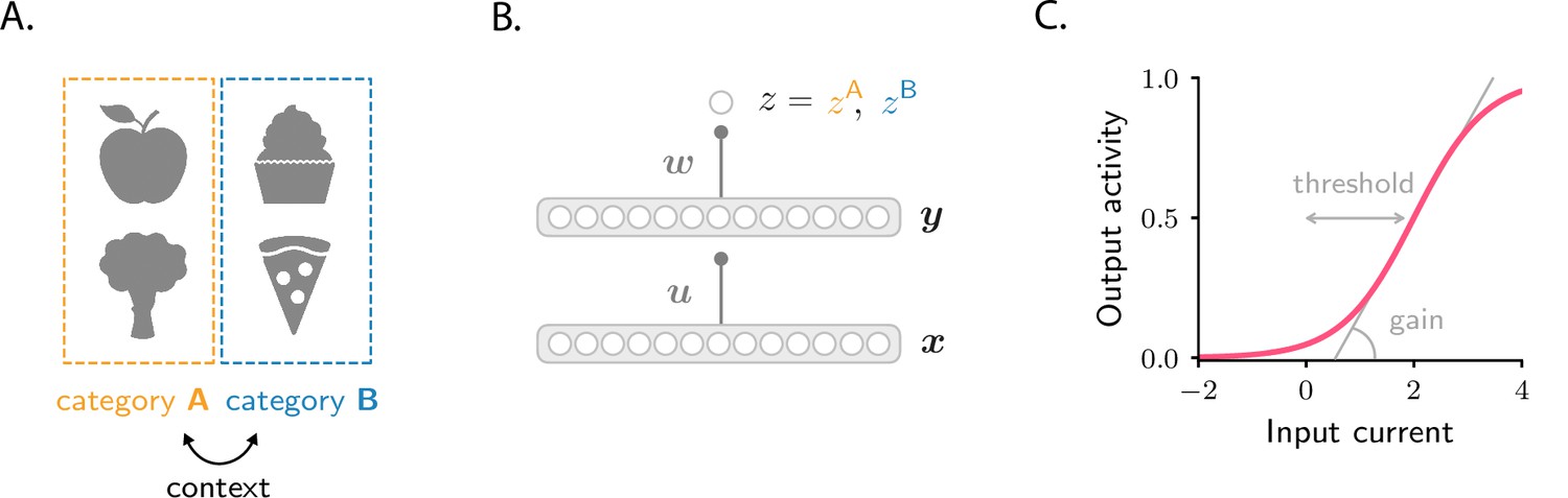
Schematics of tasks and circuit model used in the study.
(A) Illustration of the two categorization tasks. In the simple categorization task, half the stimuli are associated with category A and the other half with category B. In the context-dependent task, associations are reversed across contexts: stimuli associated with category A in context 1 are associated with category B in context 2, and vice versa. (B) The circuit consists of a sensory input layer (), an intermediate layer (), and a readout neuron (). The intermediate () and readout () weights evolve under gradient descent plasticity (Equation 1). (C) The activation functions, and , are taken to be sigmoids characterized by a threshold and a gain. The gain, which controls the sensitivity of activity to input, is the slope of the function at its steepest point; the threshold, which controls activity sparsity, is the distance from the steepest point to zero.
Figure 2 with 4 supplements
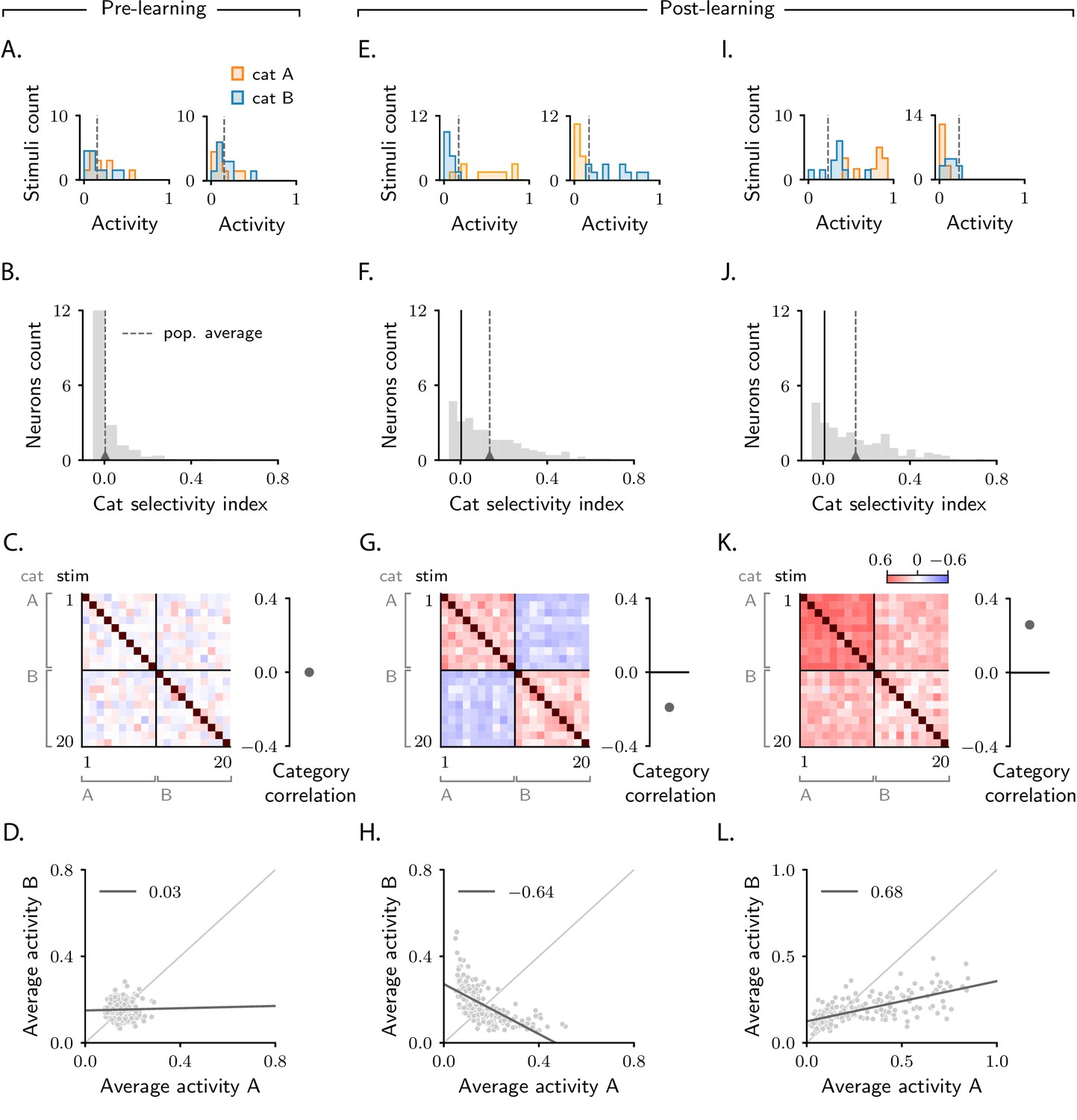
Characterization of activity evolution during the simple categorization task.
Results from simulations. The first column (A–D) shows a naive circuit (pre-learning); the second (E–H) and third (I–L) columns show two trained circuits (post-learning), characterized by different sets of parameters (see below). (A, E, I) Histograms of single-neuron activity in response to stimuli associated with category A (orange) and category B (blue). Left and right show two sample neurons from the intermediate layer. Grey dashed lines indicate the average activity across the population. (B, F, J) Histograms of category selectivity (Equation 2) across the population of neurons in the intermediate layer. Grey dashed lines indicate the average selectivity across the population. In panels F and J, the black vertical lines indicate the initial value of average selectivity. (C, G, K) Signal correlation matrices. Each entry shows the Pearson correlation coefficient, averaged over neurons (Equation 72), between activity elicited by different stimuli. In these examples, we used 20 stimuli. Diagonal entries (brown) are all equal to 1. Category correlation (namely, the average of the correlations within the off-diagonal blocks, which contain stimuli in different categories) is shown on the right of the matrices. In panels G and K, the black horizontal lines near zero indicate the initial values of category correlation. (D, H, L) Population responses to categories A and B. Each dot represents a neuron in the intermediate layer, with horizontal and vertical axes showing the responses to stimuli associated with categories A and B, respectively, averaged over stimuli. Grey line: linear fit, with Pearson correlation coefficient shown in the figure legend. Parameters are summarized in Table 1 (Materials and methods Tables of parameters).
Figure 2—figure supplement 1

Characterization of activity evolution during the simple categorization task; additional results, part I.
(A) Extensive results from simulations. Each point represents a model. We simulated 5000 different models, with parameters drawn randomly and uniformly from the following ranges: the number of stimuli, , between 10 and 30; the learning rates ratio, between 0 and 1; the gain of and between 0.05 and 1; the threshold of and between −2 and 2. Light points refer to the synaptic drive, , and dark ones to the activity, . To quantify category selectivity, we used Equation 56, and then averaged over neurons. To quantify category correlation, we used Equation 71. The vertical bars in the category correlation plots indicate the range of results obtained when quantifying correlation with the alternative definition in Equation 79. Note that selectivity changes are positive, while correlation changes take both positive and negative values. For a few parameter sets, learning convergence was pathological (i.e., the loss displayed strong oscillations over epochs, or did not converge); those cases have been excluded from the analysis. (B) Activity from circuits in Figure 2A–D (left), Figure 2E-H (center), and Figure 2I-L (right) projected on the first three principal components. Before computing the principal components, we subtracted from activity the mean across trials and neurons. Over learning, activity develops two clouds, one for each category, as schematically illustrated in Figure 3A–C. The clustering direction is approximately given by (dashed grey line). The center of the two clouds is indicated by magenta triangles; the center of initial activity is indicated by the black triangle.
Figure 2—figure supplement 2

Characterization of activity evolution during the simple categorization task; additional results, part II.
(A–D) Population response to categories A and B averaged over stimuli. Each dot represents a neuron. Panels A, B and C, D display two sample circuits, different from those displayed in Figure 2. Panels A, C and B, D display, respectively, pre- and post-learning activity. All details and parameters are as in Figure 2I–L, except: in A and B, we set the threshold of to −2; in C and D, we set the threshold of to −1.5. In panel B, in contrast to Figure 2L, the variance of activity in response to B is larger than the variance in response to A. In panel D, as in Figure 2L, the variance of activity in response to A is larger than the variance in response to B. In contrast to Figure 2L, however, the mean activity in response to B is larger than the mean activity in response to A (Materials and methods Asymmetry in category response). Note that, in all cases, category correlation remains positive. (E) Variability across circuits realizations (Materials and methods Characterizing variability): illustration from a sample circuit. Grey lines illustrate activity coordinates, , as a function of learning time, for all sensory inputs. Those were estimated by taking the dot product, and then dividing by (Equation 55 and Equation 53). Note that values corresponding to sensory inputs in the same category do not saturate to identical values; their average is indicated by dashed lines. Pink continuous lines indicate the values of and computed through the theory by neglecting variability (Equation 49). As predicted by Equation 99, the dashed and continuous pink lines do not coincide (Materials and methods Characterizing variability). (F) Activity coordinates and depend on the values of and (i.e., the input current needed by the readout neuron to to produce the target activity). For fixed targets and , those depend on the activation function . Increasing the threshold of can cause and to shift from having opposite sign to having the same sign. This in turn can cause a shift from negative to positive category correlation, see Materials and methods Simple task: category correlation.
Figure 2—figure supplement 3

Learning curves.
Behaviour of the loss function (Equation 9) over learning epochs in four sample networks. (A, B) refer to the simple categorization task; parameters are, respectively, as in Figure 2E–H and Figure 2I–L. (C, D) refer to the context-dependent categorization task; parameters are, respectively, as in Figure 6D-F and G.
Figure 2—figure supplement 4

Simple categorization task with structured inputs and heterogeneity.
Analysis of category correlation for a naive circuit (A), and two trained ones (B, C). Details are, respectively, as in Figure 2C–D, G–H and K–L. (D) Extensive analysis of average category selectivity across circuits and task parameters. Details are as in Figure 3—figure supplement 1 (except that no theory, only simulations, are shown). As in Figure 4C, D, dark and light grey indicate different values for the threshold of the activation function . Dashed lines show results obtained by subsampling pairs of sensory inputs in the category selectivity definition (Equation 56) so that initial selectivity vanishes (see Materials and methods Simple categorization task with structured inputs and heterogeneity for details). (E) Extensive analysis of category correlation across circuit and task parameters. Details as in panel D.
Figure 3 with 2 supplements
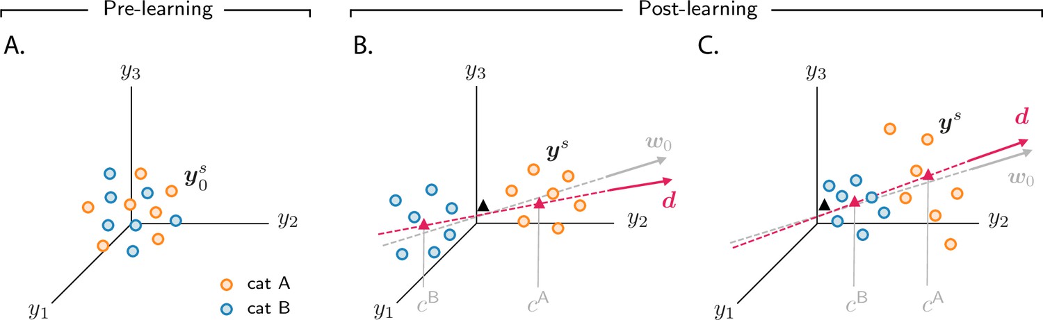
Analysis of activity evolution during the simple categorization task.
Results from mathematical analysis. (A–C) Cartoons illustrating how activity evolves over learning. The three columns are as in Figure 2: pre-learning (first column) and post-learning for two different circuits (second and third columns). Circles show activity in the intermediate layer in response to different stimuli, displayed in a three-dimensional space where axes correspond to the activity of three sample neurons. Orange and blue circles are associated, respectively, with categories A and B. Before learning, activity is unstructured (panel A). After learning (panels B and C), the activity vectors develop a component along the common direction (Equation 3), shown as a magenta line, and form two clouds, one for each category. The centers of those clouds are indicated by magenta triangles; their positions along are given, approximately, by and . The black triangle indicates the center of initial activity. In panel B, and have opposite sign, so the clouds move in opposite directions with respect to initial activity; in panel C, and have the same sign, so the clouds move in the same direction. For illustration purposes, we show a smaller number of stimuli (14, instead of 20) than in Figure 2. Simulated data from the circuits displayed in Figure 2 are shown in Figure 2—figure supplement 1B.
Figure 3—figure supplement 1

Comparison between finite-size networks and approximate mathematical description for the simple categorization task, part I.
Dashed lines show the theoretical predictions; dots show the average over 400 simulations where both the initial connectivity and the sensory inputs were drawn at random. Error bars show the standard deviation across simulations; they thus quantify variability across initializations (Materials and methods Characterizing variability). Yellow: pre-learning; gray: post-learning. (A) Activity coordinates and . Theory was computed from Equation 49. Simulations results were computed by taking the dot product for two activity vectors associated with different categories, and then dividing by (Equation 55 and Equation 53). (B) Average category selectivity. Theory was computed from Equation 66. Simulations results were computed by using Equation 56, and then averaging across neurons. We also plot results for category clustering. Theory (dotted lines) was computed from Equation 69. Simulations results (triangles) were computed by using Equation 67. Note that average selectivity and clustering are not identical for all parameters (although they become close in the limit , as discussed in Materials and methods Simple task: category selectivity). (C) Category correlation. Theory was computed from Equation 74. Simulations results were obtained by applying Equation 71 to simulated data.
Figure 3—figure supplement 2

Comparison between finite-size networks and approximate mathematical description for the simple categorization task, part II.
Details in (A-C) are as in Figure 3—figure supplement 1. We used different parameters (see Table 2), which lead to positive category correlation.
Figure 4
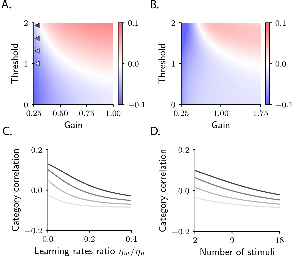
Category correlation depends on circuit and task properties.
(A) Category correlation as a function of the threshold and gain of the readout neuron. Grey arrows indicate the threshold and gain that are used in panels C and D. The learning rate ratio, , is set to 0.4 here and in panels B and D. (B) Category correlation as a function of the threshold and gain of neurons in the intermediate layer; details as in panel A. (C) Category correlation as a function of the learning rate ratio. The threshold and gain of the readout neuron are given by the triangles indicated in panel A, matched by colour. (D) Category correlation as a function of the number of stimuli; same colour code as in panel C. In all panels, correlations were computed from the approximate theoretical expression given in Materials and methods Simple task: category correlation (Equation 74). Parameters are summarized in Table 1 (Materials and methods Tables of parameters).
Figure 5
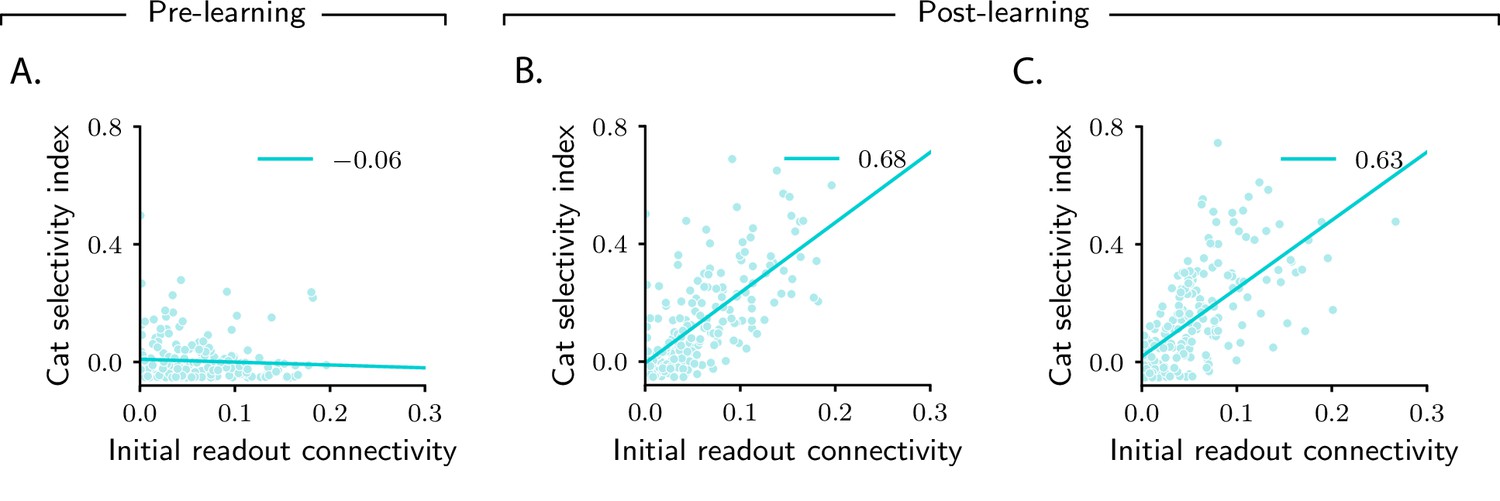
Magnitude of category selectivity depends on connectivity with the readout neuron.
(A–C) Category selectivity as a function of the initial readout connectivity (in absolute value). The three columns are as in Figure 2: pre-learning (first column) and post-learning for two different circuits (second and third columns). Each dot represents a neuron in the intermediate layer. Cyan line: linear fit, with Pearson correlation coefficient shown in the figure legend.
Figure 6 with 3 supplements

Characterization of activity evolution during the context-dependent categorization task.
Results from simulations. The first column (A–C) shows a naive circuit (pre-learning); the second (D–F) and third (G–I) columns show two trained circuits (post-learning), characterized by different sets of parameters. (A, D, G) Histogram of category selectivity (Equation 2) across the population of neurons in the intermediate layer (note that the vertical axis has been expanded for visualization purposes). Grey dashed lines indicate the average selectivity across the population. In panels D and G, the black vertical lines indicate the initial value of the average selectivity. Note that the distribution of category selectivity is different from the distribution observed in the simple task (Figure 2F, J); the distribution is now heavy tailed, with only a fraction of the neurons acquiring strong category selectivity (see also Figure 8B). (B, E, H) Histogram of context selectivity (Materials and methods Context-dependent task: category and context selectivity, Equation 122), details as in A, D, and G. (C, F, I) Correlation matrices. Each entry shows the Pearson correlation coefficient between activity from different trials. There are 8 stimuli and 8 context cues, for a total of 64 trials (i.e., 64 stimulus/context cue combinations). Diagonal entries (brown) are all equal to 1. The inset on the top of panel C shows, as an example, a magnified view of correlations among trials with context cues 1 and 8, across all stimuli (1–8). To the right of the matrices we show the context correlation, defined to be the average of the correlations within the off-diagonal blocks (trials in different contexts). In panels F and I, the black horizontal lines indicate the initial value of context correlation. Parameters are summarized in Table 1 (Materials and methods Tables of parameters).
Figure 6—figure supplement 1

Characterization of activity evolution during the context-dependent categorization task; additional results, part I.
(A) Extensive results from simulations. Each point represents a model. We simulated 5000 different models, with parameters drawn randomly. Details as in Figure 2—figure supplement 1A, except that the number of stimuli and context cues, , ranges between 4 and 20. To quantify context selectivity, we used Equation 122 and Equation 123, and then averaged over neurons. To quantify category selectivity, we used Equation 56, and then averaged over neurons. To quantify context and category correlation, we used, respectively, Equation 127 and Equation 71. The vertical bars in correlation plots indicate the range of results obtained when quantifying correlation with the alternative definitions in Equation 129 and Equation 79; for illustration purposes, the range was cut on the negative semi-axis. For a few parameter sets, learning convergence was pathological (i.e., the loss displayed strong oscillations over epochs, or did not converge); those cases have been excluded from the analysis. Note that, as in Figure 2—figure supplement 1A, selectivity changes are positive, while correlation changes take both positive and negative values. (B) Same as in A, except that changes were computed from theoretical expressions. For context selectivity, we used Equation 122 and Equation 123. For category selectivity, we used Equation 124. For context and category correlation, we used the same equations as in panel A, but evaluated them via the theoretical framework. (C, D) Activity from circuits in Figure 6A–C (left), Figure 6D-F (center) and Figure 6G-I (right) projected on the first three principal components. Details as in Figure 2—figure supplement 1B. Panels C and D display, respectively, results for the synaptic drive and the activity . The center of activity clouds for categories A and B (resp. contexts 1 and 2) is indicated by magenta (resp. pink) triangles; the center of initial activity is indicated by the black triangle.
Figure 6—figure supplement 2

Characterization of activity evolution during the context-dependent categorization task; additional results, part II.
(A, B) Population response to categories A and B, averaged over trials. Each dot represents a neuron. Panels A and B correspond to two sample circuits, characterized by different values of the threshold of the activation function . Note that responses in panel A are approximately symmetric, while those in panel B are strongly asymmetric. (C) Context dependence makes categorization more complex and causes a drop in signal correlations: extensive quantification. We computed changes in correlations for the simple and the context-dependent task across a broad range of models; details as in Figure 6—figure supplement 1B. The top panel displays the mean of correlation changes across models. Note that correlation changes are more negative in the context-dependent task. For the context-dependent task, we computed both the category and context correlation; results are displayed, respectively, in magenta and pink. In the bottom panel, we computed the fraction of models where correlation changes were positive in the simple task, and became negative in the context-dependent one (left), and vice versa (right). Note that the former substantially outnumbered the latter, which confirms that context-dependency shrinks the parameter space where changes in correlations are positive. (D) Schematic representation of the initial synaptic drive, , in the context-dependent task with (XOR). The centers of activity vectors associated with categories A and B are indicated by magenta triangles; note that the two triangles coincide exactly (Materials and methods Analysis of patterns of context and category selectivity). (E) Accuracy of a linear classifier trained to decode category from initial and final synaptic drive, and , and initial and final activity, and . Data are from the model displayed in Figure 6D–F. To train the linear classifier, we used the function svm. SVC with a linear kernel from the package sklearn; the regularization parameter was fixed through the GridSearchCV routine.
Figure 6—figure supplement 3

Characterization of activity evolution during the context-dependent categorization task; additional results, part III.
(A-B) Changes in category (panel A) and context (panel B) selectivity as a function of the components on the category and context directions, and (in absolute value). The latter are defined in Equation 167, Materials and methods Analysis of patterns of context and category selectivity. Each dot represents a neuron. Data are from the same model displayed in Figure 8. Blue line: linear fit, with Pearson correlation coefficient shown in the figure legend. Note that correlations for both panels are high. (C, D) Same analysis as in Figure 8B-C, but for the sample circuit displayed in the third column of Figure 6. (E, F) Analysis of a circuit that includes a second readout neuron, trained to report context. Panel E: circuit architecture; this is identical to the standard model (Figure 1B), except for the presence of the extra readout. All details and parameters are as in Figure 8. To make sure that the learning process associated with the two readouts drives activity changes of similar magnitude in the intermediate layer, the target values for the context readout were taken to be , . Panel F: analysis as in Figure 8B. Note that here, in contrast to Figure 8B, some neurons display a strong increase in selectivity to context, but not category (brown sample neuron).
Figure 7 with 1 supplement
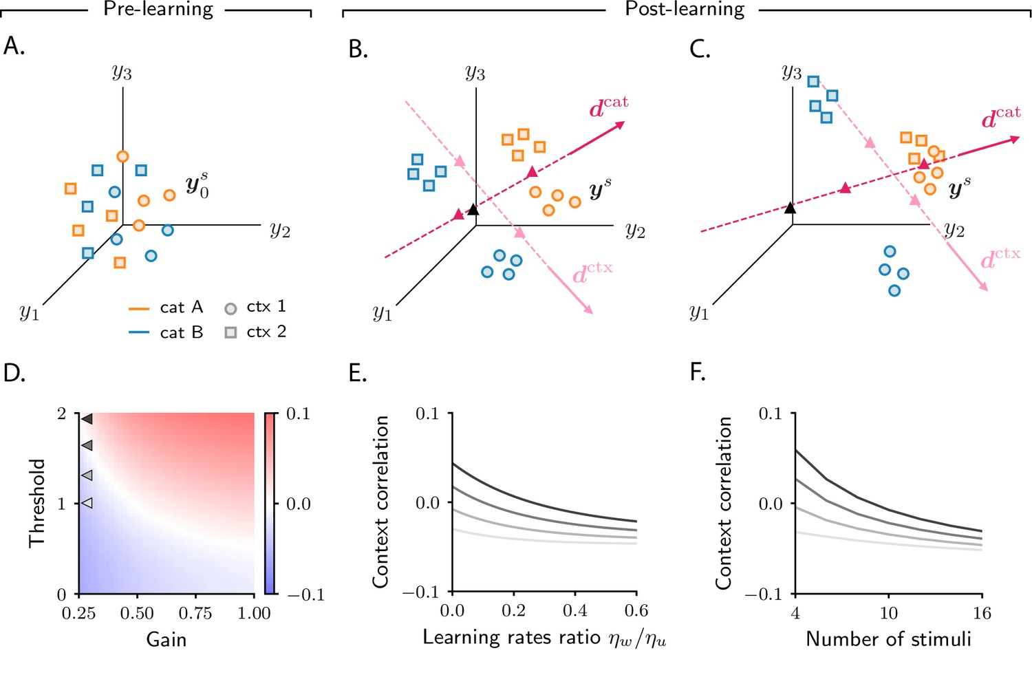
Analysis of activity evolution during the context-dependent categorization task.
Results from mathematical analysis. (A–C) Cartoons illustrating how activity evolves over learning. Orange and blue symbols are associated with categories A and B, respectively; circles and squares are associated with contexts 1 and 2. Before learning, activity is mostly unstructured (panel A). After learning, activity forms four clouds, one for each combination of category and context. The center of the activity vectors associated with categories A and B and contexts 1 and 2 are indicated, respectively, by magenta and pink triangles. The black triangle indicates the center of initial activity. The cartoons in panels A–B–C refer to the three circuits illustrated in the three columns of Figure 6; for illustration purposes, we show a reduced number of stimuli and context cues (4 instead of 8). Simulated data from the circuits displayed in Figure 6 are shown in Figure 6—figure supplement 1D. (D) Change in context correlation over learning as a function of the threshold and gain of the readout neuron. Grey arrows indicate the threshold and gain that are used in panels E and F. (E) Change in context correlation over learning as a function of the ratio of learning rates in the two layers. (F) Change in context correlation over learning as a function of the number of stimuli. Correlations in panels D–F were computed from the approximate theoretical expression given in Materials and methods Context-dependent task: category and context correlation. Parameters are given in Table 1 (Materials and methods Tables of parameters).
Figure 7—figure supplement 1

Comparison between finite-size networks and approximate mathematical description for the context-dependent categorization task.
Details are as in Figure 3—figure supplement 1. In all panels, the top and bottom plots show, respectively, results for the synaptic drive and the activity . (A) Average category selectivity. Theory was computed from Equation 124. Simulations results were computed by using Equation 56, and then averaging across neurons. We also plot results for category clustering (triangles); clustering was computed by applying Equation 124 to simulated data. (B) Average context selectivity. Theory was computed from Equation 125. Simulations results were computed by using Equation 122, and then averaging across neurons. Context clustering was computed from Equation 125. (C) Context correlation. Theory was computed from Equation 127. Simulations results were obtained applying Equation 127 to simulated data. (D–F) Details as in A–C. We used different parameters (see Table 2), which lead to positive changes in context correlation.
Figure 8
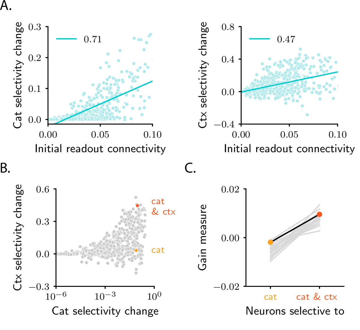
Patterns of pure and mixed selectivity to category and context.
(A) Changes in category selectivity (left) and context selectivity (right) as a function of the initial readout connectivity, (in absolute value). Details as in Figure 5B, C. (B) Changes in context selectivity as a function of changes in category selectivity. Note the logarithmic scale on the -axis; this is required by the heavy-tailed behaviour of category selectivity (Figure 6D, G). We highlighted two sample neurons: one with strong, pure selectivity to category (yellow) and one with strong, mixed selectivity to category and context (orange). (C) Neurons that develop pure and mixed selectivity are characterized by different patterns of initial activity. Here, we plot the gain-based measure of activity defined in Equation 183 for neurons that belong to the former (left), and the latter (right) group. The former group includes neurons for which the change in category selectivity, but not the change in context selectivity, is within the top 15% across the population. The latter group includes neurons for which the change in both category and context selectivity is within the top 15%. Dots show results for the circuit analyzed in panels A and B. Grey lines show results for 20 different circuit realizations; note that the slope is positive for all circuits. All panels in the figure show results for the circuit displayed in the second column of Figure 6; the circuit displayed in the third column yields qualitatively similar results (Figure 6—figure supplement 3C, D).
Tables
Table 1
Table of parameters for figures in the main text.
| Figure | |||||||
|---|---|---|---|---|---|---|---|
| Figures 2, 3 and 5, first and second columns | 200 | 20 | 0.0 | 1.0 | 2.0 | 1.0 | 0.0 |
| Figures 2, 3 and 5, third column | 200 | 20 | 0.0 | 1.0 | 2.0 | 1.0 | 2.0 |
| Figure 4A | 200 | 20 | 0.4 | 2.0 | 2.0 | varies | varies |
| Figure 4B | 200 | 20 | 0.4 | varies | varies | 1.0 | 2.0 |
| Figure 4C | 200 | 20 | varies | 2.0 | 2.0 | 1.0 | varies |
| Figure 4D | 200 | varies | 0.4 | 2.0 | 2.0 | 1.0 | varies |
| Figure 6A–C, first and second columns | 600 | 8 (P = 64) | 0.0 | 1.0 | 0.0 | 1.0 | 0.0 |
| Figure 6A–C, third column | 600 | 8 (P=64) | 0.0 | 1.0 | 0.0 | 1.0 | 4.0 |
| Figure 7D | 600 | 8 (P = 64) | 0.2 | 2.5 | 2.0 | varies | varies |
| Figure 7E | 600 | 8 (P = 64) | varies | 2.5 | 2.0 | 1.0 | varies |
| Figure 7F | 600 | varies | 0.2 | 2.5 | 2.0 | 1.0 | varies |
Table 2
Table of parameters for figure supplements.
| Figure supplement | |||||||
|---|---|---|---|---|---|---|---|
| Figure 2—figure supplement 1A | 200 | varies | varies | varies | varies | varies | varies |
| Figure 2—figure supplement 2E | 200 | 20 | 0.0 | 1.0 | 2.0 | 1.0 | 0.0 |
| Figure 3—figure supplement 1, first column | varies | 20 | 0.0 | 1.0 | 0.0 | 1.0 | 0.0 |
| Figure 3—figure supplement 1, second column | 200 | 20 | varies | 1.0 | 0.0 | 1.0 | 0.0 |
| Figure 3—figure supplement 1, third column | 200 | 20 | 0.0 | 1.0 | varies | 1.0 | 0.0 |
| Figure 3—figure supplement 2, first column | varies | 20 | 0.0 | 1.0 | 0.0 | 1.0 | 2.0 |
| Figure 3—figure supplement 2, second column | 200 | 20 | varies | 1.0 | 0.0 | 1.0 | 2.0 |
| Figure 3—figure supplement 2, third column | 200 | 20 | 0.0 | 1.0 | varies | 1.0 | 2.0 |
| Figure 2—figure supplement 4A, B | 200 | 12 | 0.0 | 1.0 | 2.0 | 1.0 | 0.0 |
| Figure 2—figure supplement 4C | 200 | 12 | 0.0 | 1.0 | 2.0 | 1.0 | 2.0 |
| Figure 2—figure supplement 4D, E, first column | 200 | 12 | 0.1 | 2.0 | varies | 1.0 | varies |
| Figure 2—figure supplement 4D, E, second column | 200 | 12 | varies | 2.0 | 2.0 | 1.0 | varies |
| Figure 2—figure supplement 4D, E, third column | 200 | varies | 0.1 | 2.0 | 2.0 | 1.0 | varies |
| Figure 6—figure supplement 1A, B | 600 | varies | varies | varies | varies | varies | varies |
| Figure 6—figure supplement 2A | 600 | 8 (P = 64) | 0.0 | 1.0 | 3.0 | 1.0 | 0.0 |
| Figure 6—figure supplement 2B | 600 | 8 (P = 64) | 0.0 | 1.0 | 3.0 | 1.0 | 4.0 |
| Figure 6—figure supplement 2C | 600 | varies | varies | varies | varies | varies | varies |
| Figure 7—figure supplement 1A–C | 600 | varies | 0.0 | 1.0 | 0.0 | 1.0 | 0.0 |
| Figure 7—figure supplement 1D–F | 600 | varies | 0.0 | 1.0 | 0.0 | 1.0 | 4.0 |
Additional files
Download links
A two-part list of links to download the article, or parts of the article, in various formats.
Downloads (link to download the article as PDF)
Open citations (links to open the citations from this article in various online reference manager services)
Cite this article (links to download the citations from this article in formats compatible with various reference manager tools)
Evolution of neural activity in circuits bridging sensory and abstract knowledge
eLife 12:e79908.
https://doi.org/10.7554/eLife.79908


