Figures and data in Evolution of cell size control is canalized towards adders or sizers by cell cycle structure and selective pressures

Version of Record: November 11, 2022
Accepted Manuscript: September 30, 2022

Download
A two-part list of links to download the article, or parts of the article, in various formats.
Downloads (link to download the article as PDF)
- Article PDF
Open citations (links to open the citations from this article in various online reference manager services)
- Mendeley
Cite this article (links to download the citations from this article in formats compatible with various reference manager tools)
Felix Proulx-Giraldeau

Jan M Skotheim

Paul François

(2022)
Evolution of cell size control is canalized towards adders or sizers by cell cycle structure and selective pressures

eLife 11:e79919.

https://doi.org/10.7554/eLife.79919
- Download BibTeX
- Download .RIS
Cite
Share
CommentOpen annotations (there are currently 0 annotations on this page).

Figures
Tables
Additional files

17 figures, 8 tables and 1 additional file

Figures

Figure 1

Download asset Open asset

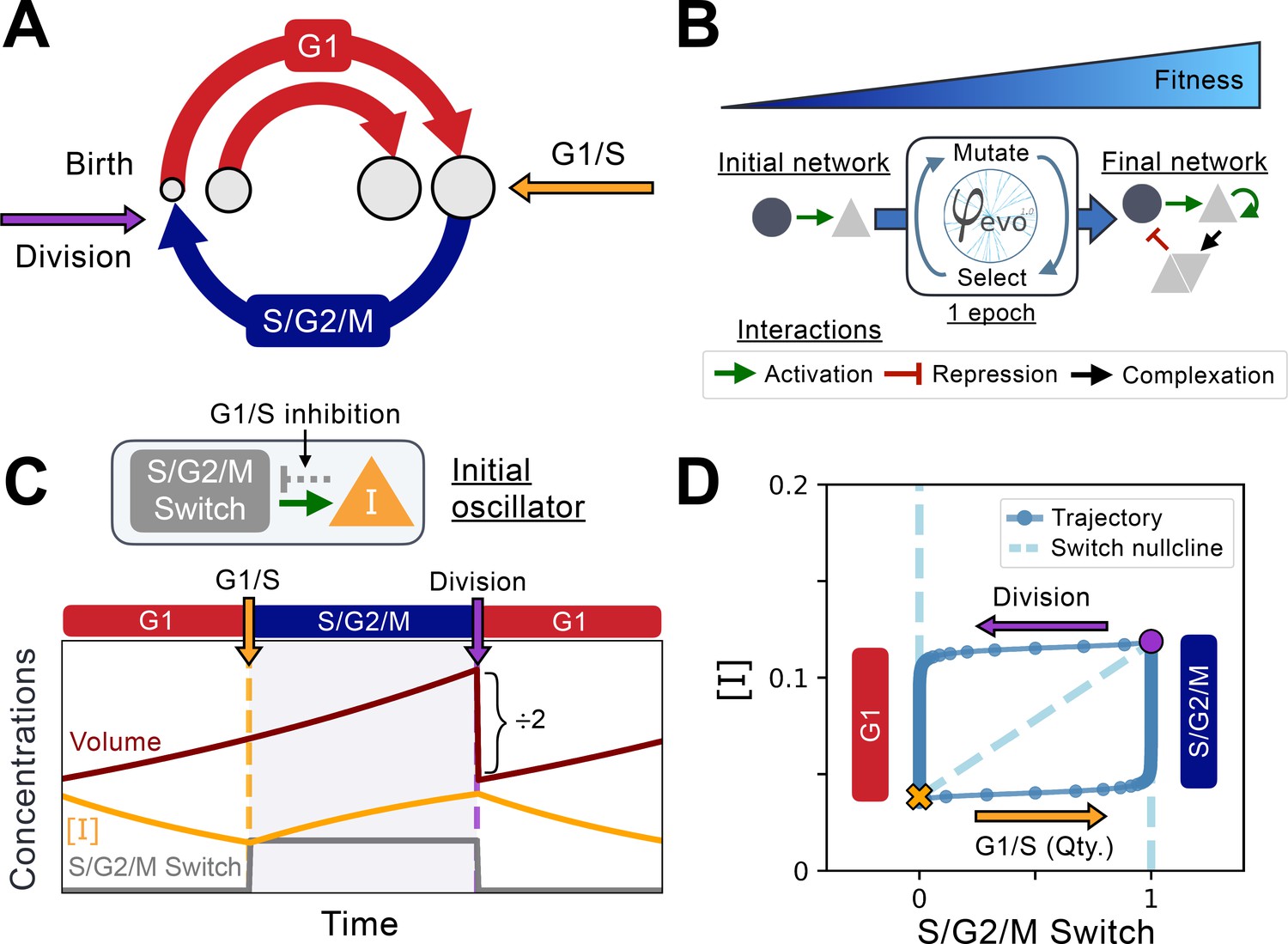
Implementation of the cell cycle seed network and evolution algorithm.

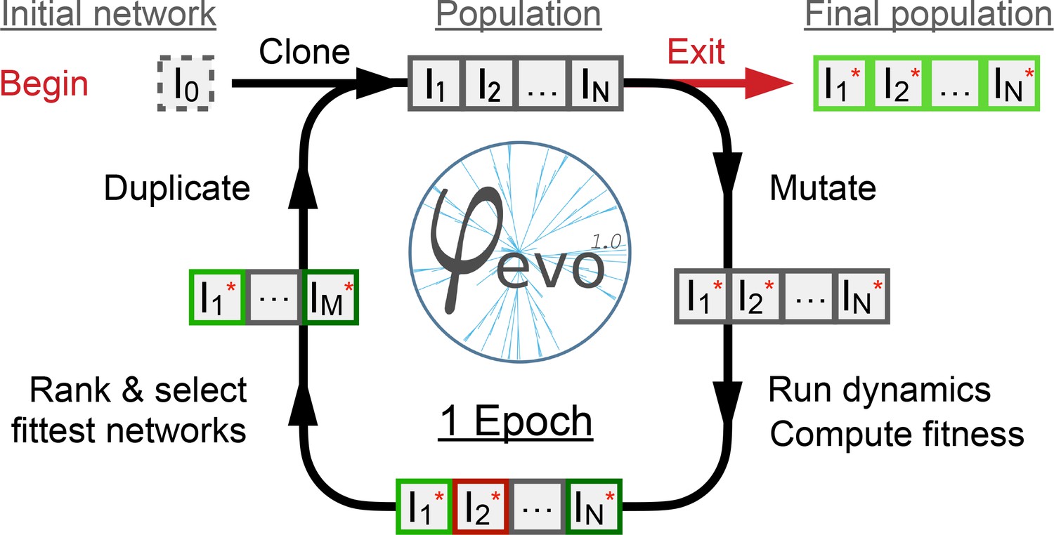
(A) Schematic representation of the coupling between cell size and cell cycle progression. The transition between G1 (red) and S phases of the cell cycle at the G1/S transition (orange) can evolve …

Figure 2

Download asset Open asset

Evolution of feedback-based size control.

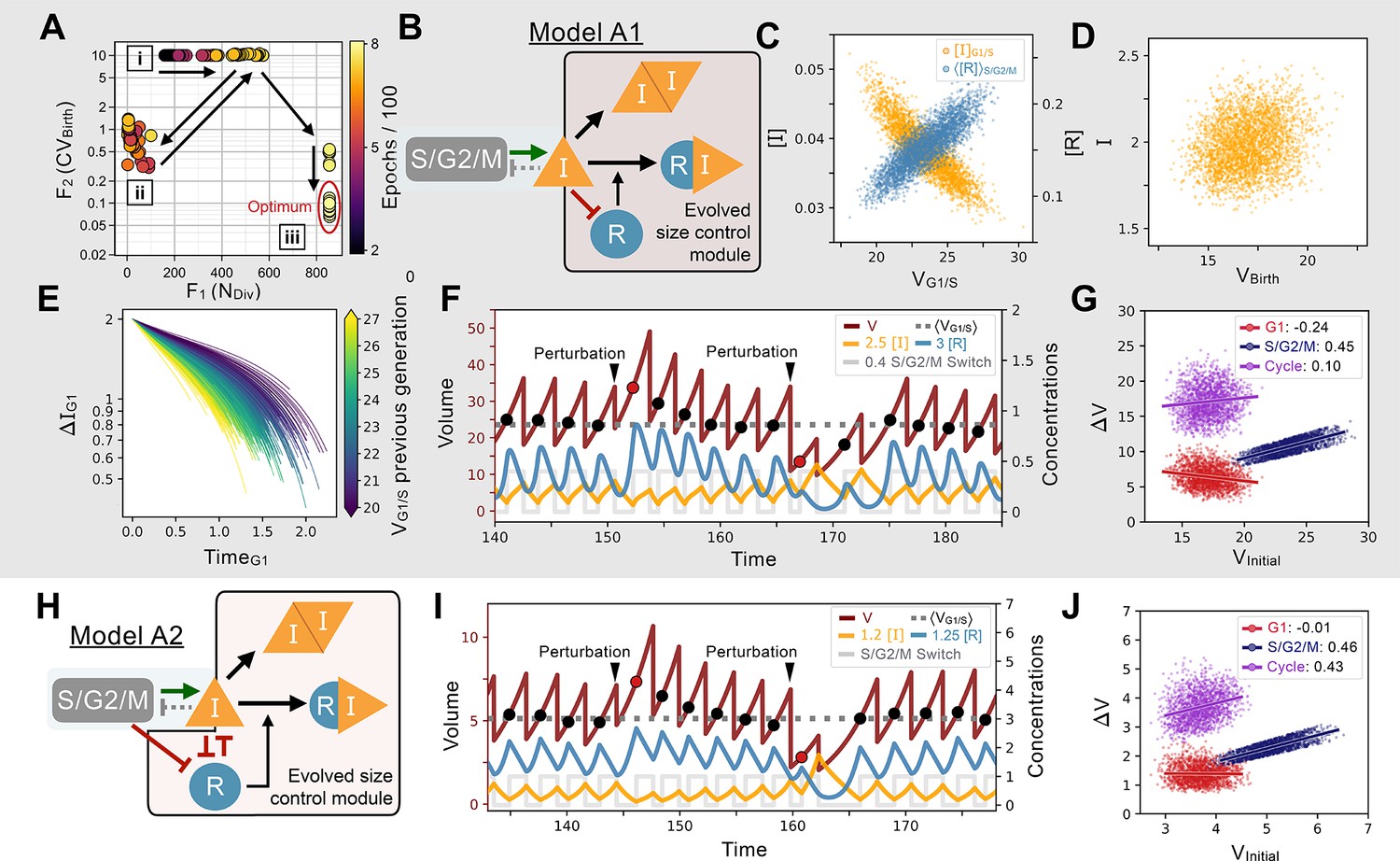
(A) Typical 2D fitness trajectory for an evolutionary run. Individual networks are dots color coded by their epoch within the evolutionary trajectory. Fitness function of the number of divisions of …

Figure 3

Download asset Open asset

Characterizing and comparing evolved size control mechanisms.

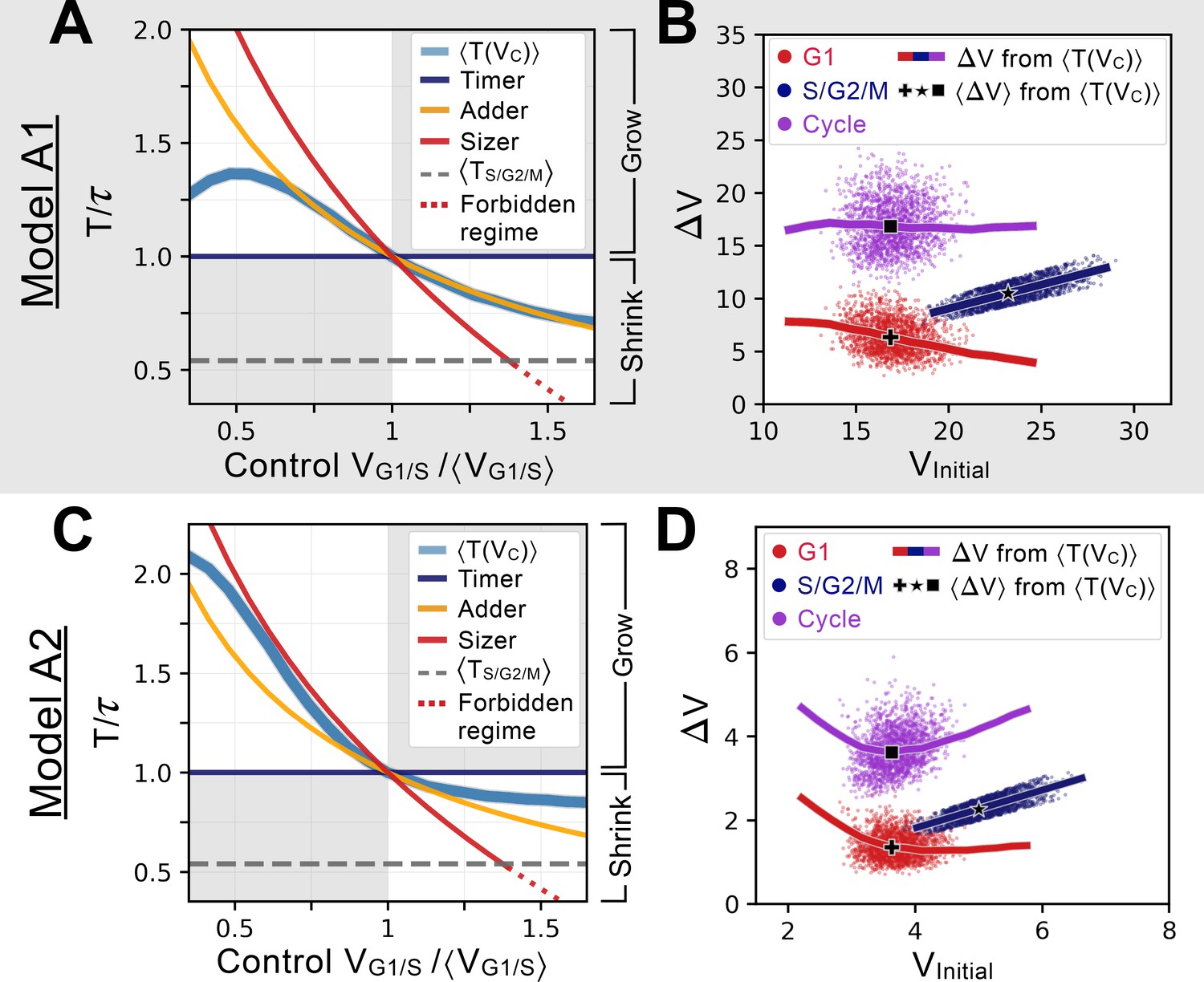
(A) Average period $T (V_{C})$ of the oscillator of Model A1 as a function of the control volume $V_{C}$ at the G1/S transition. Period is normalized by $τ$ the doubling time of the cell, and volume is rescaled by …

Figure 4

Download asset Open asset

Distinct network constraints and selection pressures bias size control evolution towards adders or sizers.

Summary statistics for evolutionary simulations each having 500 epochs. Model A1 shown in Figure 2A-G was used as the initial seed network. 60 simulations were performed using Pareto optimization of …

Figure 5

Download asset Open asset

System and evolutionary dynamics of cell size control networks.

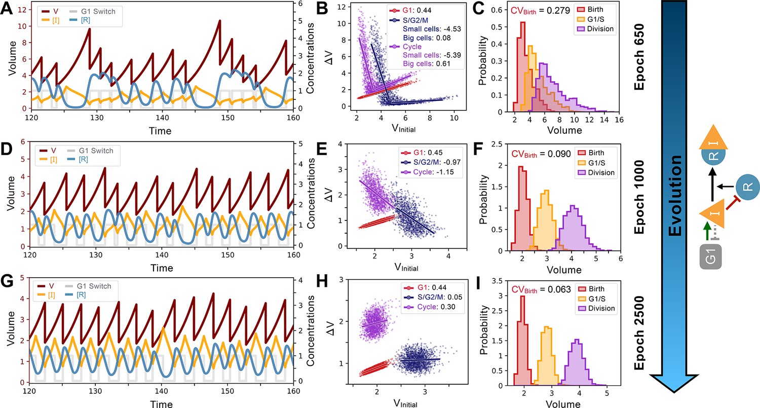
Snapshots of an evolutionary simulation of 2500 epochs initialized with the Model A1 network topology along with an *S. pombe*-like cell cycle structure with a timer in G1 followed by a sizer in …

Figure 6

Download asset Open asset

An evolved concentration fluctuation sensing size control model exhibits self-organized criticality.

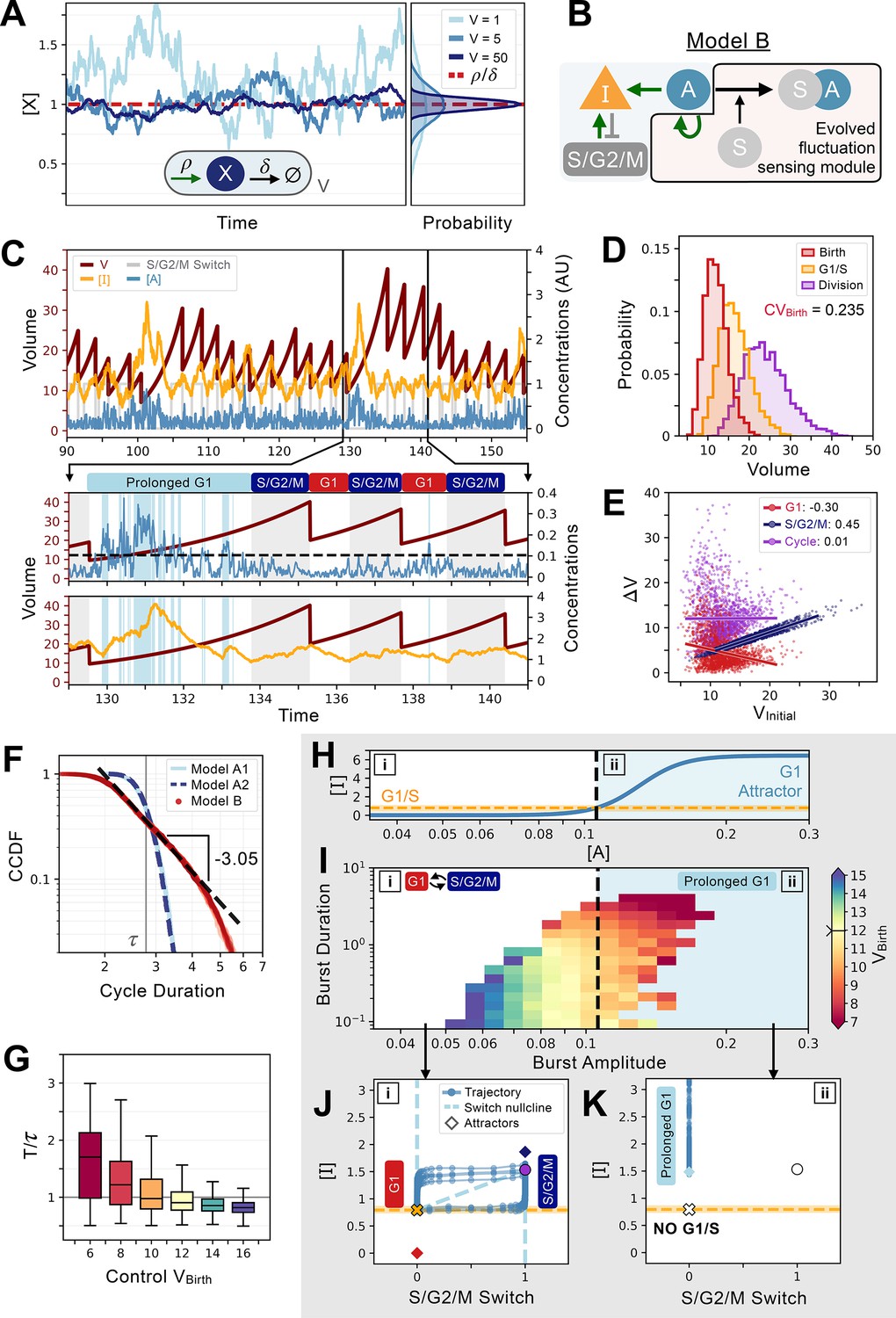
(A) Size-dependent molecular noise arises due to Poissonian fluctuations in molecule number. Consider a protein production-degradation scheme for protein *quantity X* with production rate $ρ$ and …

Appendix 1—figure 1

Download asset Open asset

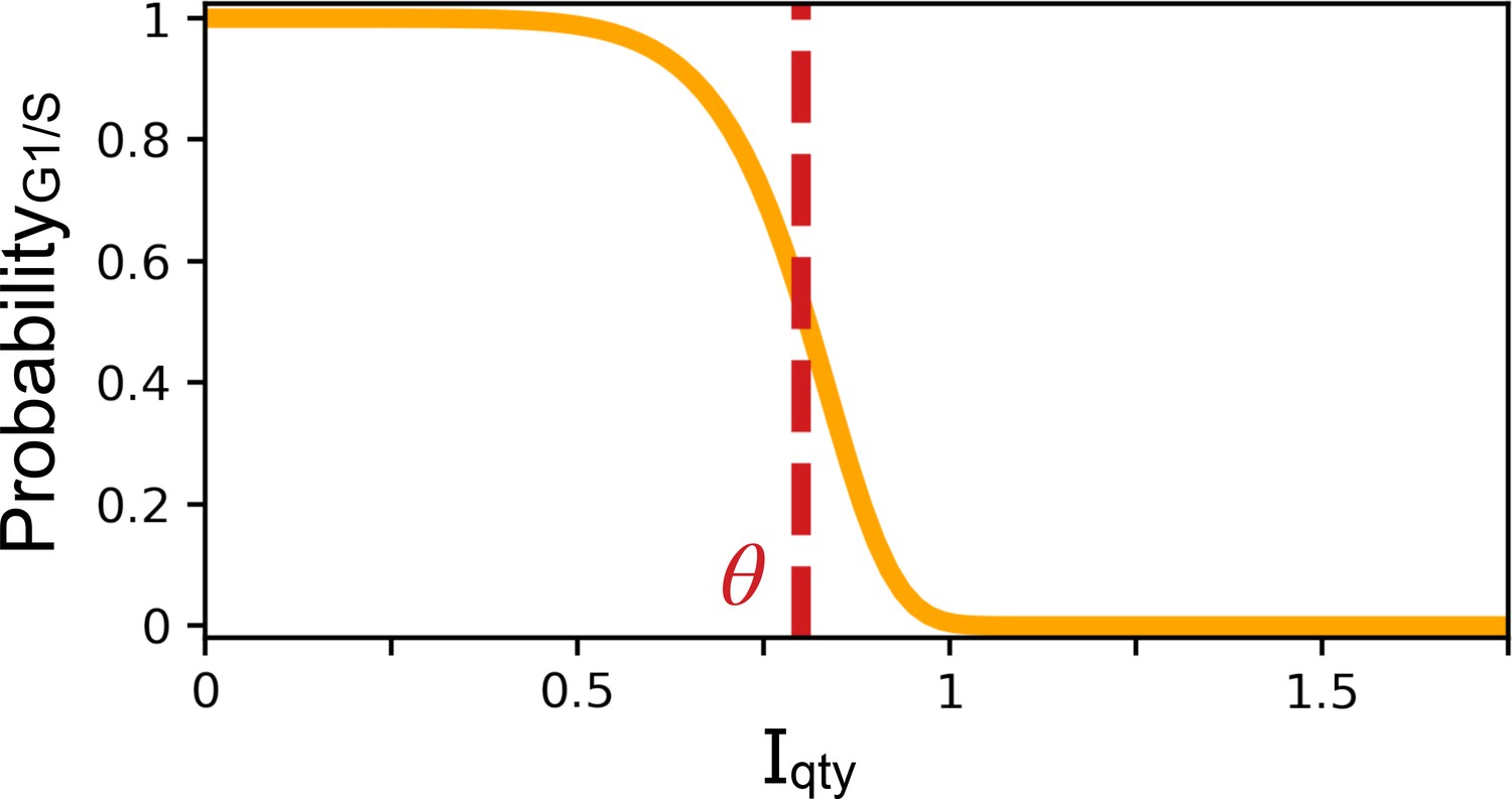
Probability of the G1/S transition occurring at the next time step.

X-coordinate is the quantity of the transcriptional regulator $I$ . Y-coordinate is the probability of the G1/S transition occurring at the next time step $Δ t$ . Parameters $θ = 0.8$ and $n_{θ} = 8$ .

Appendix 1—figure 2

Download asset Open asset

Control volume and archetype response curves.

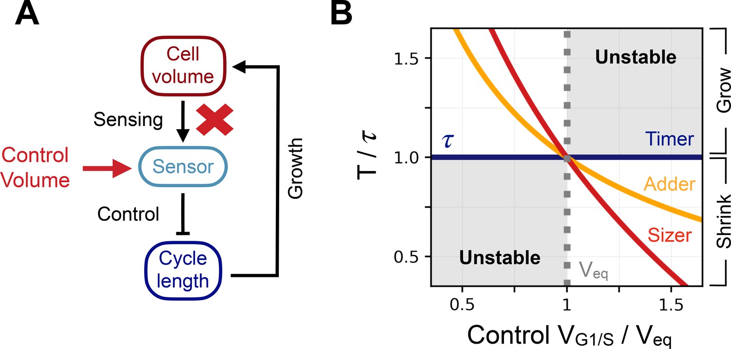
(A) Schematic representation of the way we break the feedback in the system and impose a control volume $V_{C}$ (red arrow) at the G1/S transition in order to record the induced cell cycle period $T (V_{C})$ . (B) …

Appendix 1—figure 3

Download asset Open asset

Response curves for the initial seed networks.

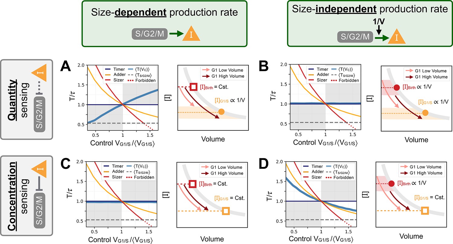
Columns indicate the size scaling assumption of the protein production rates as indicated above the figure. Rows indicate quantity or concentration sensing of inhibitor $I$ at the G1/S transition …

Appendix 1—figure 4

Download asset Open asset

Schematic representation of the $φ$ -evo algorithm.

We begin with a user-defined initial seed network as starting point of the evolutionary process. The seed network is cloned to give a first population of networks. Individuals are then mutated …

Appendix 1—figure 5

Download asset Open asset

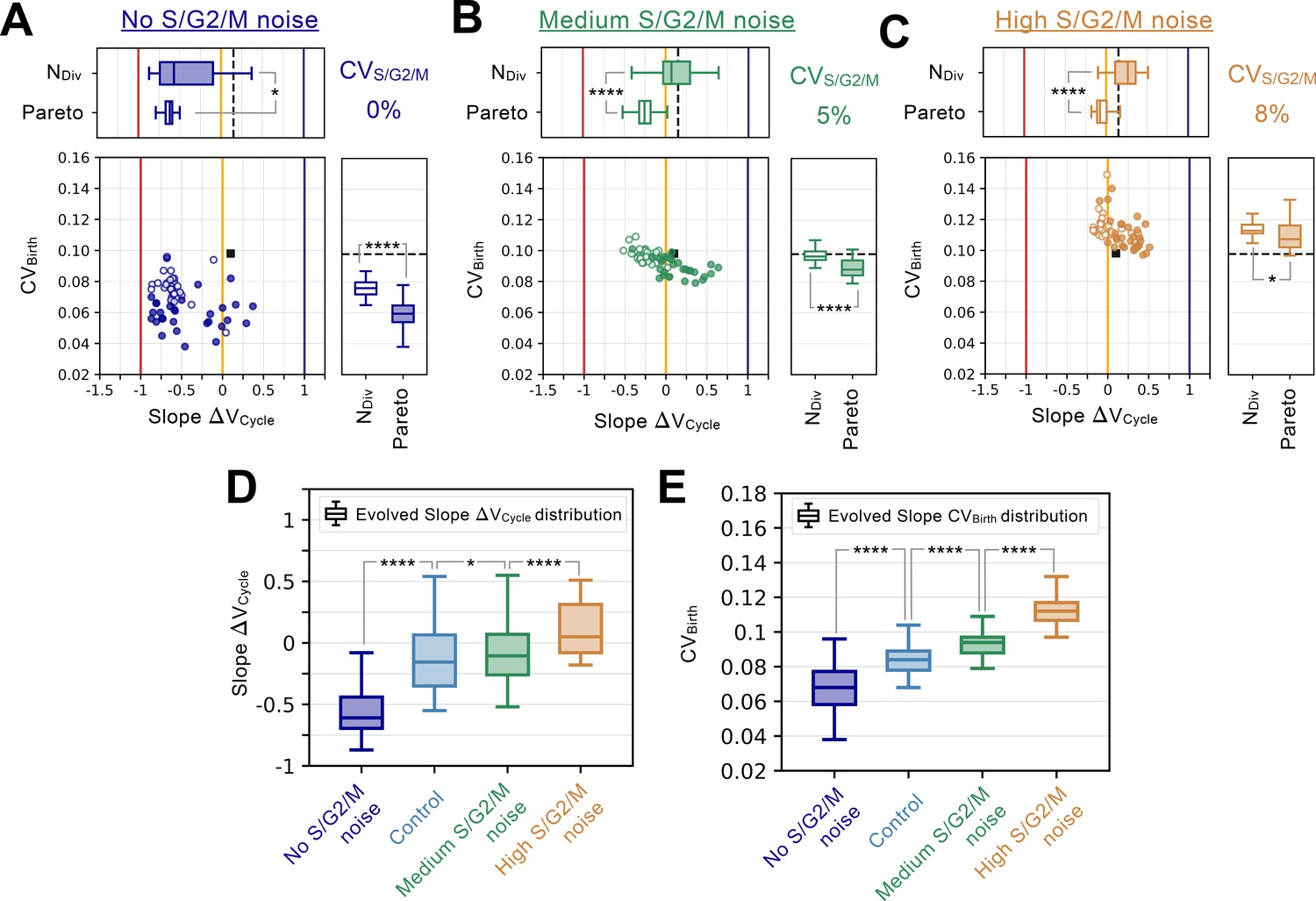
S/G2/M noise analysis.

Summary statistics for evolutionary simulations each having 500 epochs. Model A1 was used as the initial seed network. 30 simulations were performed using Pareto optimization of the number of …

Appendix 1—figure 6

Download asset Open asset

Growth rate noise analysis.

Summary statistics for evolutionary simulations each having 500 epochs. Model A1 was used as the initial seed network. Only 30 simulations were performed using Pareto optimization of the number of …

Appendix 1—figure 7

Download asset Open asset

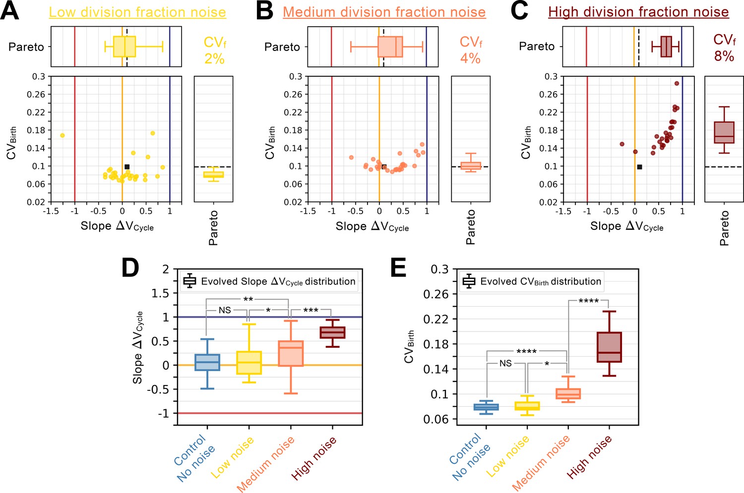
Division fraction noise analysis.

Summary statistics for evolutionary simulations each having 500 epochs. Model A1 was used as the initial seed network. Only 30 simulations were performed using Pareto optimization of the number of …

Appendix 1—figure 8

Download asset Open asset

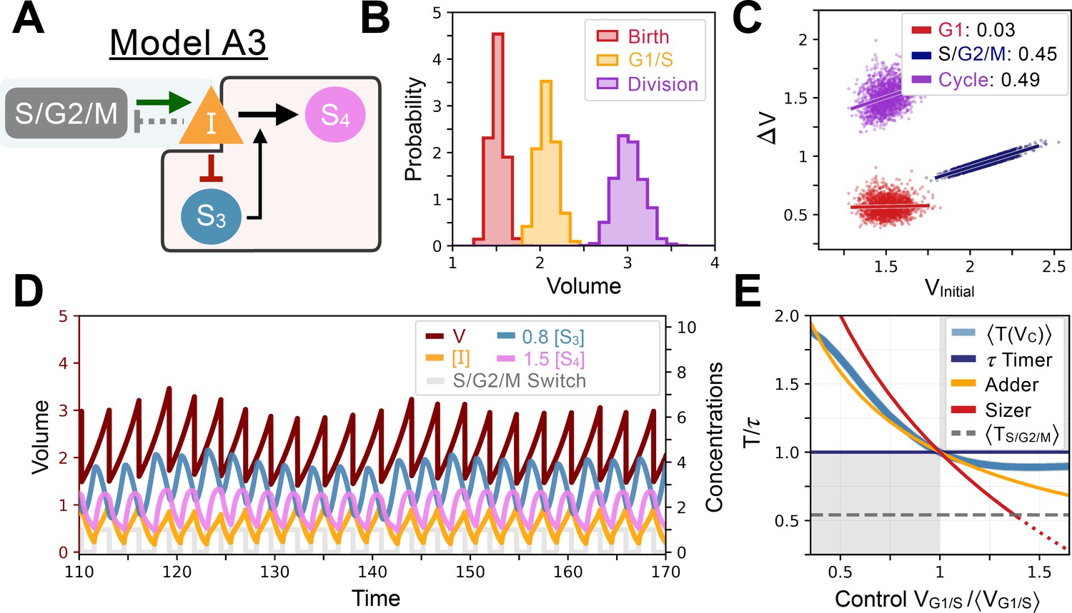
Model A3’s behavior.

(A) Network topology of the evolved Model A3. S₃ is as a size sensor and titrates $I$ in a size-dependent manner. (B) Size distributions at birth (red), G1/S (orange), and division (purple). (C) …

Appendix 1—figure 9

Download asset Open asset

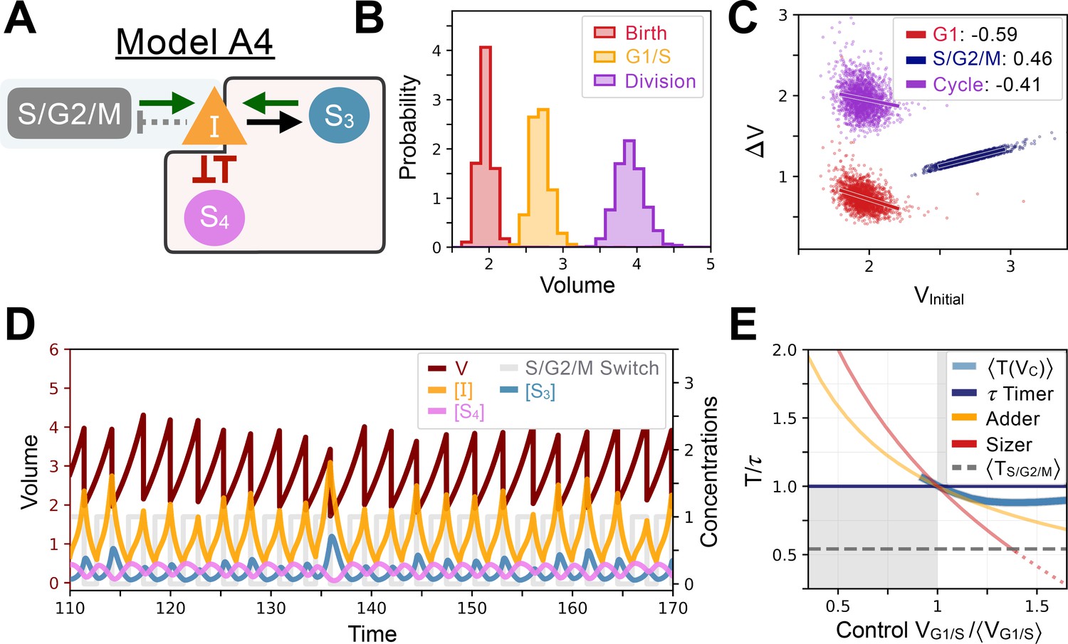
Model A4’s behavior.

(A) Network topology of the evolved Model A4. S₄ is the size sensor and represses the production of $I$ in a size-dependent manner. (B) Size distributions at birth (red), G1/S (orange) and division …

Appendix 1—figure 10

Download asset Open asset

Model A5’s behavior.

(A) Network topology of the evolved Model A5. S₃ is the size sensor and represses the production of $I$ in a size-dependent manner. (B) Size distributions at birth (red), G1/S (orange) and division …

Appendix 1—figure 11

Download asset Open asset

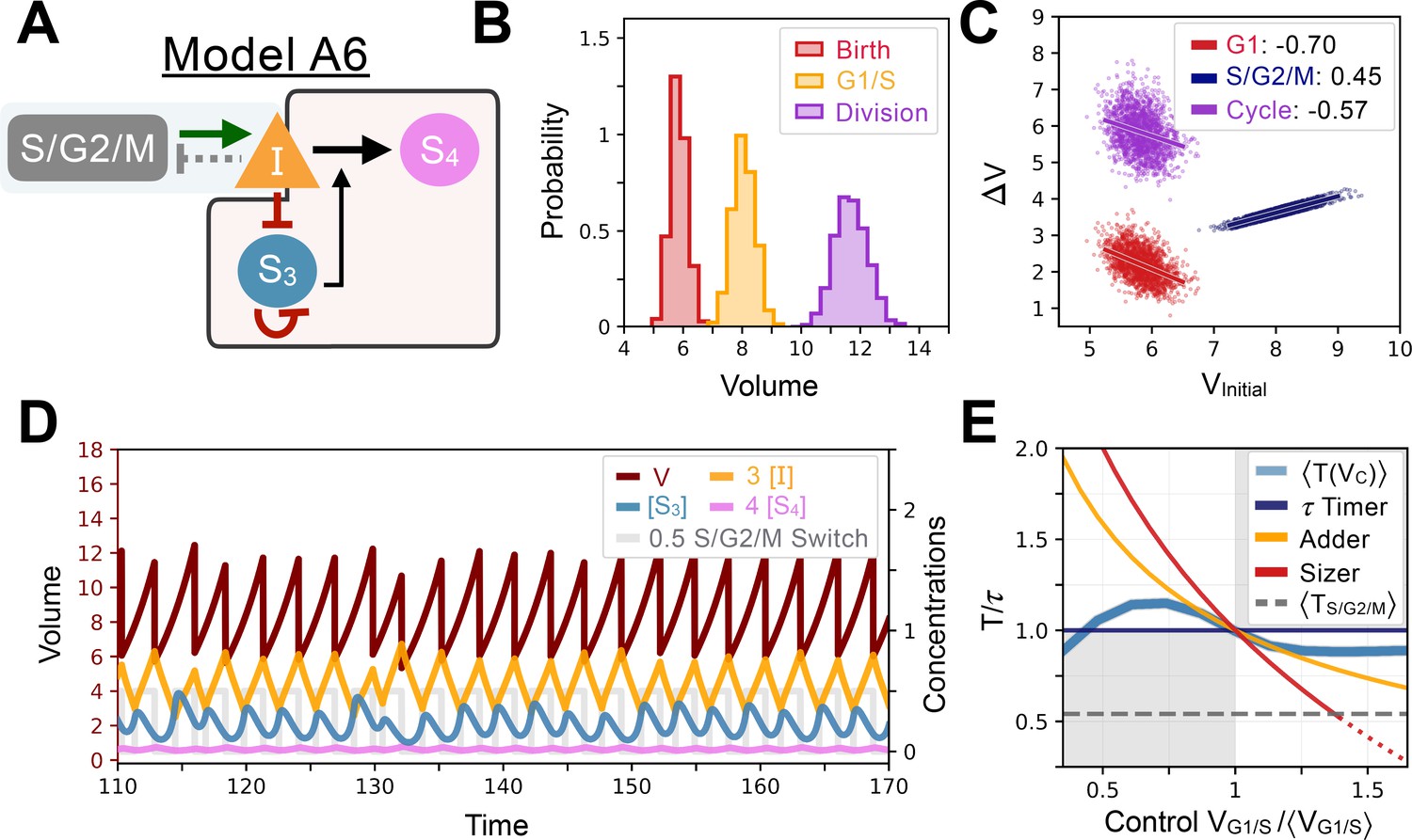
Model A6’s behavior.

(A) Network topology of the evolved Model A6. S₃ is the size sensor and represses the production of $I$ in a size-dependent manner. (B) Size distributions at birth (red), G1/S (orange) and division …

Tables

Appendix 1—table 1

Coefficients of variation: models and experiments.

Models		Data
Name	$C V_{Birth}$	Cell type	Time of size measure	$C V$
A1	0.098	Haploid budding yeast	Budding	0.17
A2	0.095	Haploid fission yeast	Fission	0.06
B	0.235	Mouse epidermal stem cell	Birth	0.17

Appendix 1—table 2

Model A1 parameter values.

Parameter	Value	Parameter	Value
p₂	0.369408	$δ_{3}$	0.4574764
$t_{1 : 2}$	1.104619	$k_{f 1}$	6.783001
$n_{1 : 2}$	3.215727	$k_{b 1}$	0.195168
$δ_{2}$	0.083827	$δ_{4}$	4.244007
p₃	0.703658	$k_{f 2}$	0.021174
$t_{2 : 3}$	0.044938	$k_{b 2}$	1.075146
$n_{2 : 3}$	3.266732	$δ_{5}$	1.1010876

Appendix 1—table 3

Model A2 parameter values.

Parameter	Value	Parameter	Value
$p_{2}$	1.915601	$n_{1 : 3}$	2.751652
$t_{1 : 2}$	0.17872	$t_{2 : 3}$	0.441106
$n_{1 : 2}$	2.09054	$n_{2 : 3}$	2.780297
$t_{3 : 2}$	0.962612	$δ_{3}$	0.045051
$t_{3 : 2}$	2.144666	$k_{f 1}$	0.839879
$δ_{2}$	0.019495	$k_{b 1}$	0.381067
$p_{3}$	1.944803	$δ_{4}$	0.913992
$t_{1 : 3}$	0.422939	0

Appendix 1—table 4

Model B parameter values.

Parameter	Value	Parameter	Value
p₂	4.968896	$n_{3 : 3}$	3.189190
$t_{1 : 2}$	2.569361	$δ_{3}$	0.246561
$n_{1 : 2}$	0.952178	p₄	4.674459
$t_{3 : 2}$	0.131057	$δ_{4}$	1.010978
$n_{3 : 2}$	9.219961	k_f	3.194116
$δ_{2}$	0.521437	k_b	4.634009
p₃	0.113586	$δ_{5}$	1.165439
$t_{3 : 3}$	2.183079	C₀	1

Appendix 1—table 5

Model A3 parameter values.

Parameter	Value	Parameter	Value
p₂	5.606156	$t_{2 : 3}$	1.410420
$t_{1 : 2}$	0.066136	$n_{2 : 3}$	3.434213
$n_{1 : 2}$	8.177965	k_f	1.930909
b₂	0.911279	k_b	3.871610
$δ_{2}$	0.257920	$δ_{3}$	0.013294
p₃	5.887584	$δ_{4}$	1.803926

Appendix 1—table 6

Model A4 parameter values.

Parameter	Value	Parameter	Value
p₂	5.6604334	$δ_{2}$	0.001059
$t_{1 : 2}$	0.408208	k_f	0.843408
$n_{1 : 2}$	1.769233	k_b	1.680321
$t_{3 : 2}$	0.887392	$δ_{3}$	0.825150
$n_{3 : 2}$	6.437683	p₄	4.674459
$t_{4 : 2}$	0.197495	$t_{2 : 4}$	0.744119
$n_{4 : 2}$	3.238633	$n_{2 : 4}$	3.451469
b₂	0.800255	$δ_{4}$	1.929584

Appendix 1—table 7

Model A5 parameter values.

Parameter	Value	Parameter	Value
p₂	2.379635	b₄	2.624939
$t_{1 : 2}$	0.142770	$δ_{4}$	1.499653
$n_{1 : 2}$	0.383384	$δ_{5}$	0.006318
$t_{3 : 2}$	0.714386	$δ_{6}$	0.983140
$n_{3 : 2}$	8.642875	$δ_{7}$	0.481592
$t_{4 : 2}$	1.754776	$k_{f 1}$	0.226150
$n_{4 : 2}$	7.783080	$k_{b 1}$	3.793388
b₂	0.195855	$k_{f 2}$	1.608325
$δ_{2}$	0.576282	$k_{b 2}$	3.322565
b₃	0.582449	$k_{f 3}$	2.999118
$δ_{3}$	0.318466	$k_{b 3}$	0.906997

Appendix 1—table 8

Model A6 parameter values.

Parameter	Value	Parameter	Value
p₂	0.369408	$δ_{2}$	0.093159
$t_{1 : 2}$	0.748731	$k_{f 1}$	0.533415
$n_{1 : 2}$	3.850889	$k_{b 1}$	3.141514
p₃	3.868044	$δ_{3}$	0.626507
$t_{2 : 3}$	0.082081	$k_{f 2}$	3.911233
$n_{2 : 3}$	3.638939	$k_{b 2}$	1.885120
$t_{3 : 3}$	0.599375	$δ_{4}$	0.821609
$n_{3 : 3}$	6.300643	$δ_{5}$	1.882484