Coding of latent variables in sensory, parietal, and frontal cortices during closed-loop virtual navigation
- Center for Neural Science, New York University, United States
- Center for Theoretical Neuroscience, Columbia University, United States
Figures
Figure 1
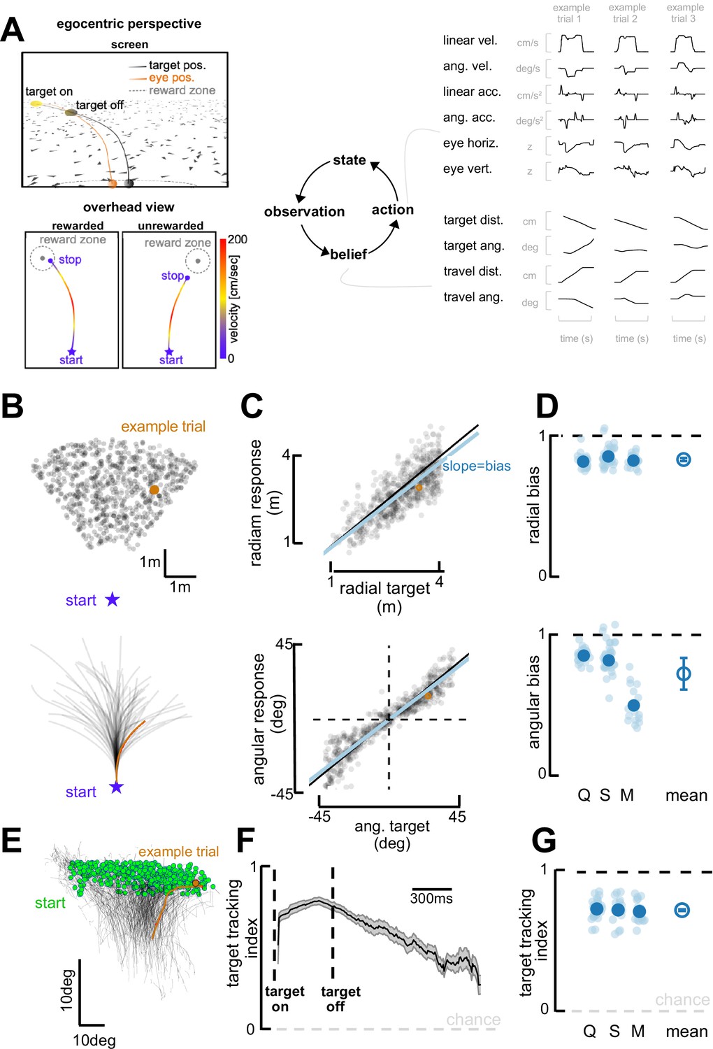
Task and behavioral results.
(A) Behavioral task. Top left: Egocentric perspective of the monkey during the firefly task, emphasizing the ground plane optic flow elements (flashing triangles), the fact that the target disappears (target off), and eye positions (following target position perfectly when the target is on, and then continuing on the correct path but deviating with time). Bottom left: Overhead view of the monkey, starting location (star), accelerating and progressively re-orienting to face the firefly, before de-accelerating and stopping at (left; rewarded) or near (right: unrewarded) the location of the now invisible target. Right: This task involves making observation of the sensory environment (composed of optic flow), using these observations to generate a dynamic belief (of the relative distance to target), and producing motor commands based on the current belief, which in turn updates the state of the environment. Right: Continuous variables are shown for three example trials. (B) Top: spatial distribution of target positions across trials. Bottom: monkey trajectories. The orange dot and trajectory are an example trial, maintained throughout the figure. (C) Example session. Radial (top) and angular (bottom) endpoint (y-axis) as a function of target (x-axis). Gray dots are individual trials, black line is unity, and blue line is the regression between response and target (slope of 1 indicates no bias). (D) Radial (top) and angular (bottom) bias (slope,=1 means no bias, >1 means overshooting, and <1 means undershooting) for every session (transparent blue circles) and monkey (x-axis, dark blue circles are average for each monkey, Q, S, and M). Rightmost circle is the average across monkeys and error bars represent ±1 SEM. Overall, monkeys are fairly accurate but undershoot targets, both radially and in eccentricity. (E) Eye trajectories (green = eye position at firefly offset) for an example session, projected onto a two-dimensional ‘screen’. Eyes start in the upper field and gradually converge in the lower center (where the firefly ought to be when they stop). (F) Target-tracking index (variance in eye position explained by prediction of fixating on firefly) for an example session as a function of time since firefly onset and offset. (G) Average target-tracking index within 1 s for all sessions (light blue) and monkeys (dark blue) showing the monkeys attempt to track the invisible target.
Figure 2 with 11 supplements
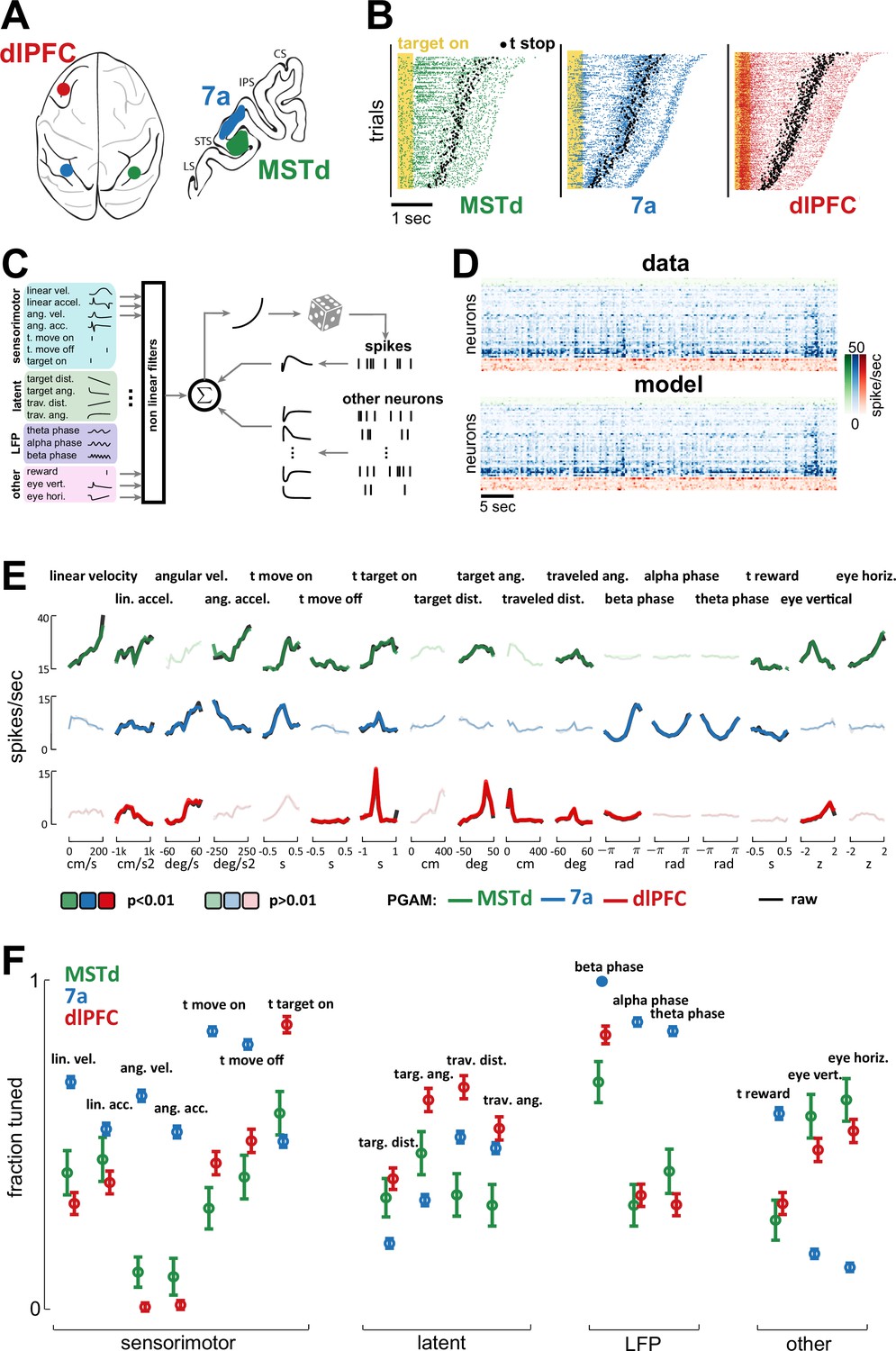
Dorsomedial superior temporal area (MSTd), area 7a, and dorsolateral prefrontal cortex (dlPFC) encode a heterogeneous mixture of task variables.
(A) Schematic of brain areas recorded. (B) Raster plots of spiking activity in MSTd (green), 7a (blue), and dlPFC (red). Shaded yellow area represents the time of the target being visible, and black dots represent the timing of movement offset. Trials are sorted from shortest (bottom) to longest (top) duration of the trial. (C) Schematic of the Poisson generalized additive model (P-GAM) used to fit spike trains. The task and neural variables used as input to the model were: linear and angular velocity and acceleration, time of movement onset and offset, time of firefly onset, distance and angle from origin and to target, time of reward, vertical and horizontal position of the eyes, and ongoing phase of LFP at theta, alpha, and beta bands. (D) Top: random snippet of spiking activity of simultaneously recorded neurons (green = MSTd; blue = 7a; red = dlPFC). Bottom: corresponding cross-validated prediction reconstructed from the P-GAM. The average cross-validated pseudo-R2 was 0.072 (see Colin Cameron and Windmeijer, 1997). (E) Responses from an example MSTd, 7a, and dlPFC neuron (black), aligned to temporal task variables (e.g., time of movement onset and offset), or binned according to their value in a continuous task variable (e.g., linear velocity). Colored (respectively green, blue, and red for MSTd, 7a, and dlPFC) lines are the reconstruction from the reduced P-GAM. The responses are opaque (p<0.01) or transparent (p>0.01), according to whether the P-GAM kernel for the specific task variable is deemed to significantly contribute to the neuron’s firing rate. (F) Fraction of neurons tuned to the given task variable, according to brain area. Error bars are 99% CIs, and thus non-overlapping bars indicate a pair-wise significant difference.
Figure 2—figure supplement 1
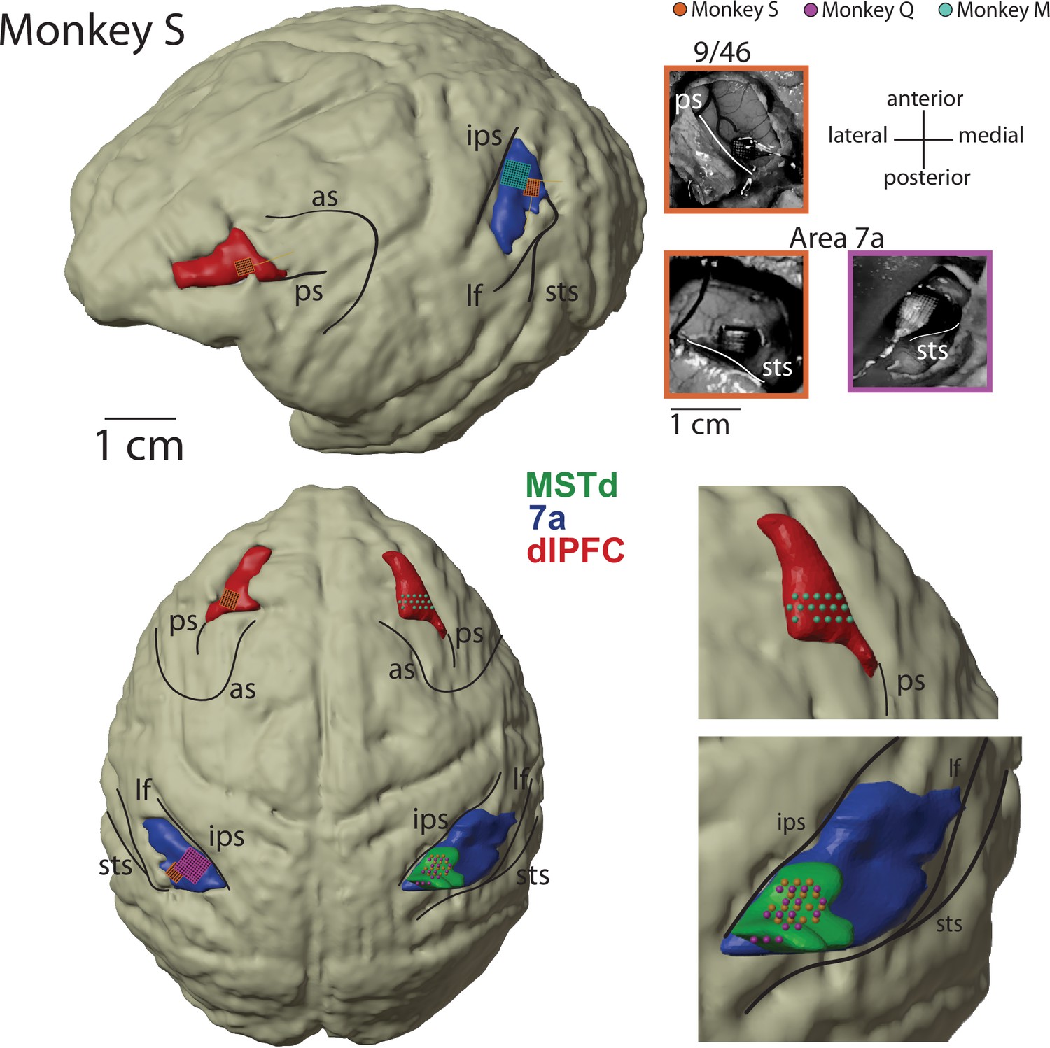
Recoding sites.
Magnetic resonance imaging (MRI) reconstruction of recording sites and pictures from Utah array implants. 3D rendering of the brain is from Monkey S, and all recording sites have been placed on the common reference (dorsomedial superior temporal area [MSTd] in green, area 7a in blue, dorsolateral prefrontal cortex [dlPFC] in red). Location of acute recordings are indicated by spheres, color coded per animal (Monkey S, orange; Monkey Q, purple; Monkey M in green). Location of Utah arrays are indicated by squares. The pictures of the Utah arrays are framed in the color corresponding to the monkey. In turn, Monkey S had recordings performed from Utah arrays in dlPFC and area 7a on the left hemisphere, and from a linear probe in MSTd on the right hemisphere. Monkey Q had recordings performed from a Utah array in 7a on the left hemisphere and from a linear probe in MSTd on the right hemisphere. Monkey M had recordings performed from a linear probe in dlPFC on the right hemisphere. In total, therefore, each area was sampled twice. All 7a recordings were on the left hemisphere and all MSTd recordings were on the right hemisphere (note, given that MSTd is directly ventral to 7a, see Figure 2A, these cannot be recorded from the same hemisphere if the former area is implanted with an array). From the 823 neurons recorded in dlPFC, 55 were recorded on the right hemisphere in Monkey M. All inter-area coupling analyses (which requires simultaneous recordings) were based on left-hemisphere recordings in 7a and dlPFC, and from right-hemisphere recordings in MSTd. All monkeys were right-handed and used this hand to manipulate the joystick. AS, arcuate sulcus; IPS, intraparietal sulcus; PS, principal sulcus; STS, superior temporal sulcus; LF, lateral fissure.
Figure 2—figure supplement 2
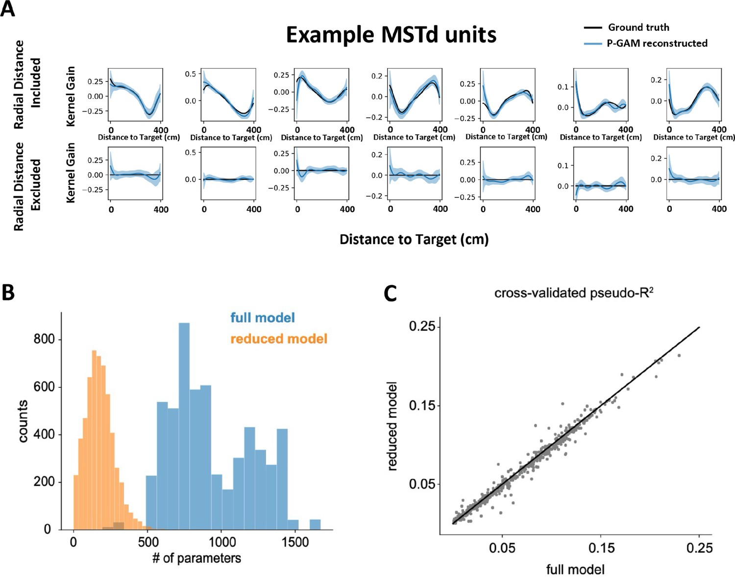
Poisson generalized additive model (P-GAM) controls.
(A) Feature inclusion in the ‘reduced’ model. We generated synthetic spike trains according to real input statistics (e.g., linear and angular velocity profiles, correlated inputs) and tuning functions derived in dorsomedial superior temporal area (MSTd) by the P-GAM (all 17 variables, as in the main text). Next, we attempted to recover these tuning functions, while including or excluding (i.e., zeroing) the tuning to radial distance to target. Across all simulation (n=1344), the P-GAM never excluded the distance to target from its selected model when this variable had not been zeroed (0.0% false negative), and only once failed to exclude this variable from its final selection when the variable had been zeroed (0.0007% false positive). Top row are significant tuning functions to radial distance in MSTd (black) and their recovered shape by the P-GAM (blue) when not excluded. Bottom row are the same units when radial distance (but not other variables) was zeroed. Columns show seven example cells. (B) Number of parameters in the ‘full’ and ‘reduced’ model. The full model is the model with all parameters, before any selection is applied. The reduced model is the model where only parameters relating to features that significantly contribute to a neuron’s spiking are kept. By design, the reduced model ought to have an equal or lower number of parameters than the full model. The full model number of parameters varies, according to how many simultaneously recorded neurons there were in a recording session, given that we include unit-to-unit coupling terms. (C) Cross-validated pseudo-R2 in the full and reduced model. While the reduced model has on average 18.9% the number of parameters as in the full model (B) its ability to account for neural activity is comparable to the full model.
Figure 2—figure supplement 3
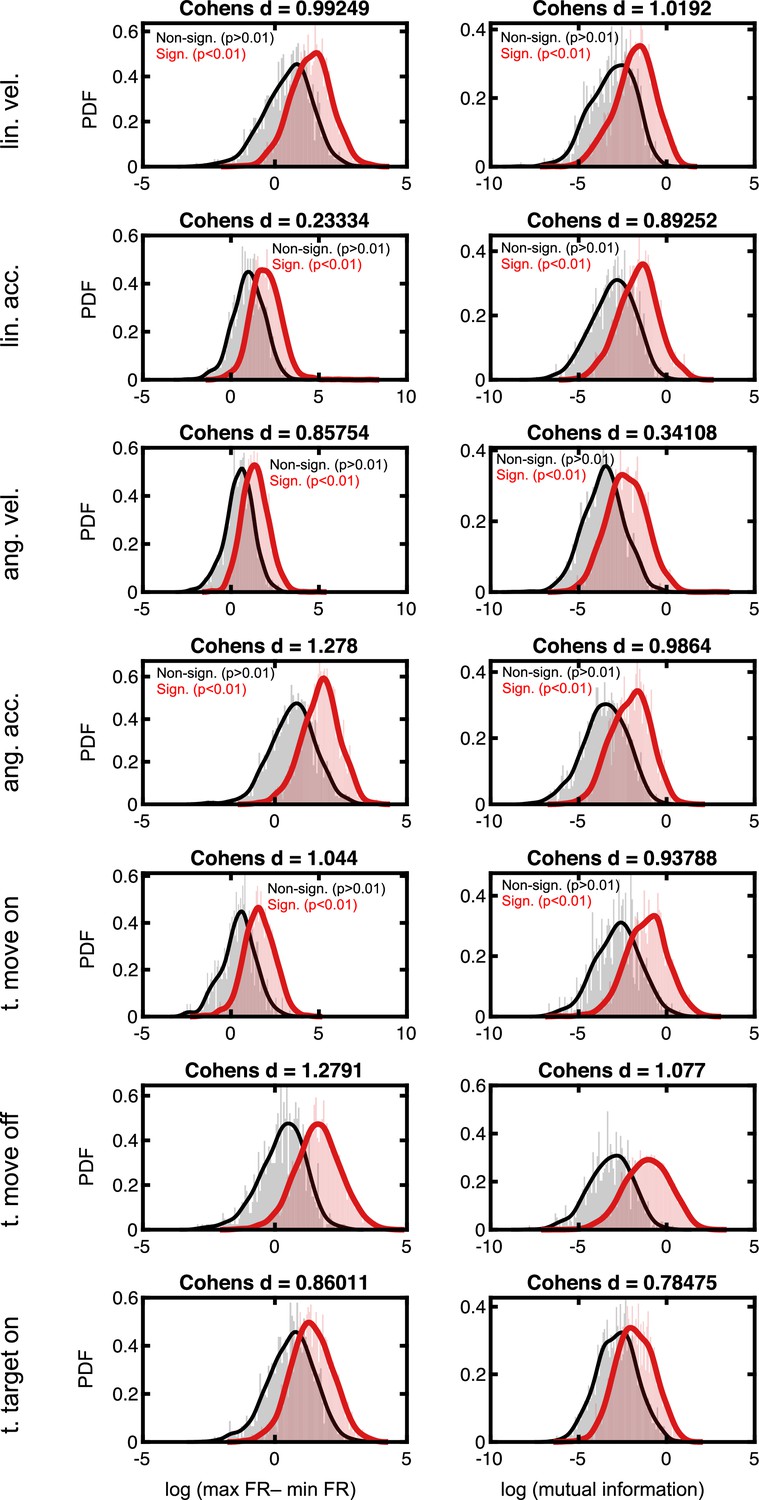
Effect sizes in the firing rate space for neurons deemed to code for sensorimotor variables.
Rows are the different sensorimotor variables, in the same order as in Figure 2E and F. The left column is the difference in evoked firing rate between the population of neurons deemed to significantly code for, or not, a given task variable. Namely, for each neuron we compute the difference in firing rate between the peak and the trough of its tuning function. The populations of significant and non-significant neurons are then log-transformed (to render normally distributed) and Cohen’s d is computed (indicated as the title of each subplot). Right column, as for the left column, but while contrasting the mutual information present between firing rates and the given task variable. For reference, Cohen’s d < ~0.2 are typically considered weak effects, ~0.5 are considered moderate, and >~0.8 are considered strong effects.
Figure 2—figure supplement 4
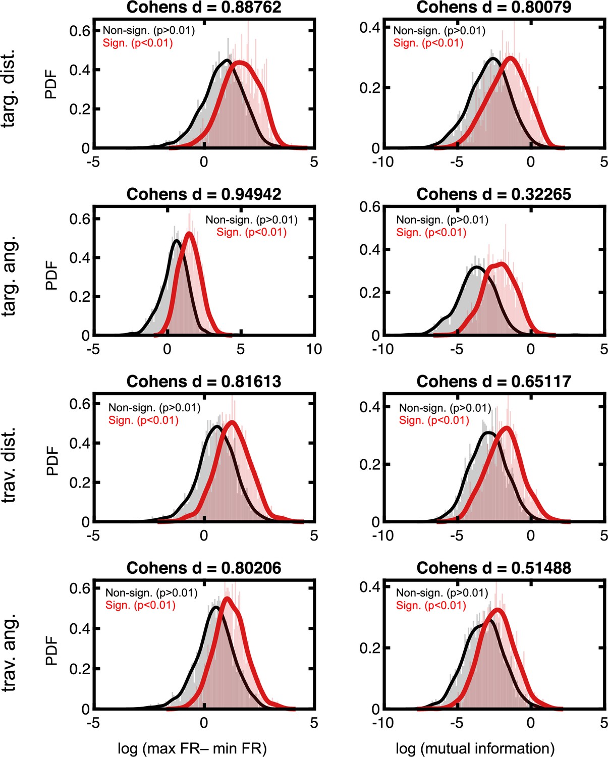
Effect sizes in the firing rate space for neurons deemed to code for latent variables.
Format follows that of Figure 2—figure supplement 3.
Figure 2—figure supplement 5
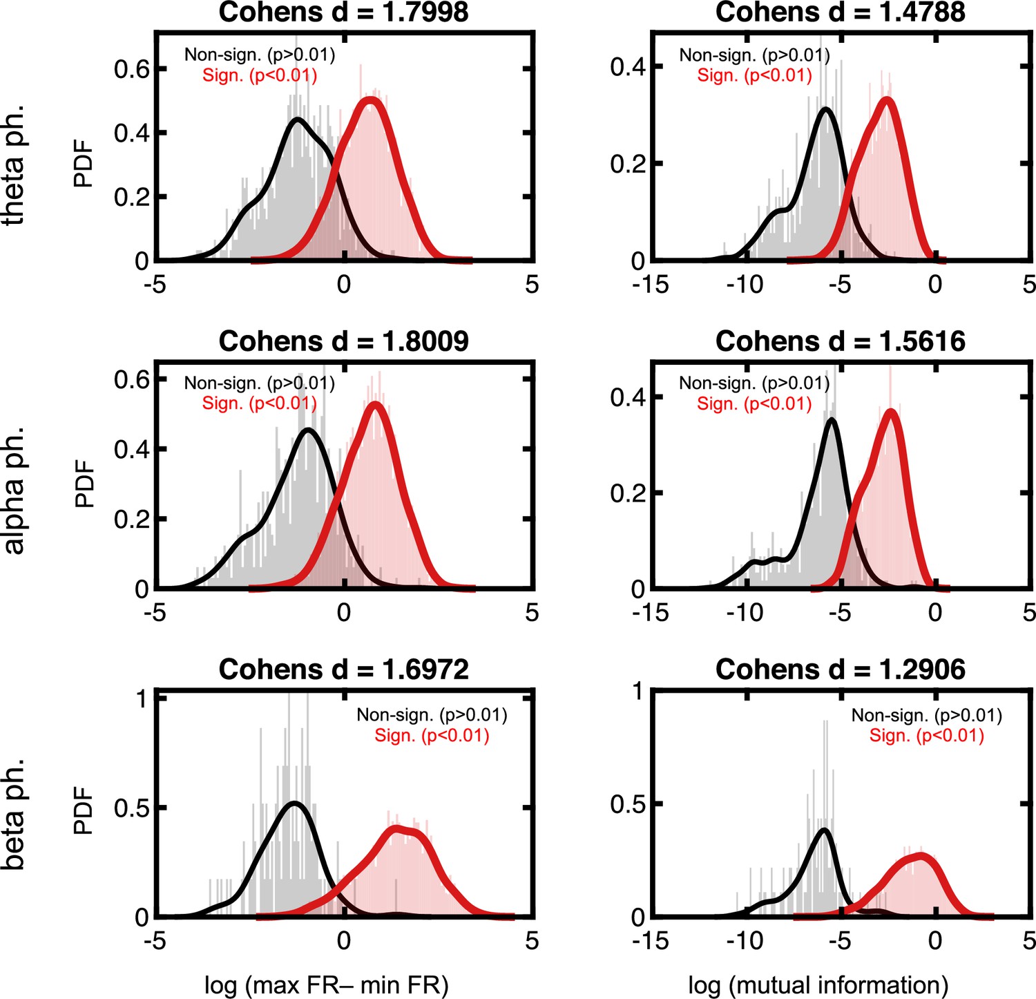
Effect sizes in the firing rate space for neurons deemed to phase lock to local field potential (LFP).
Format follows that of Figure 2—figure supplement 3.
Figure 2—figure supplement 6
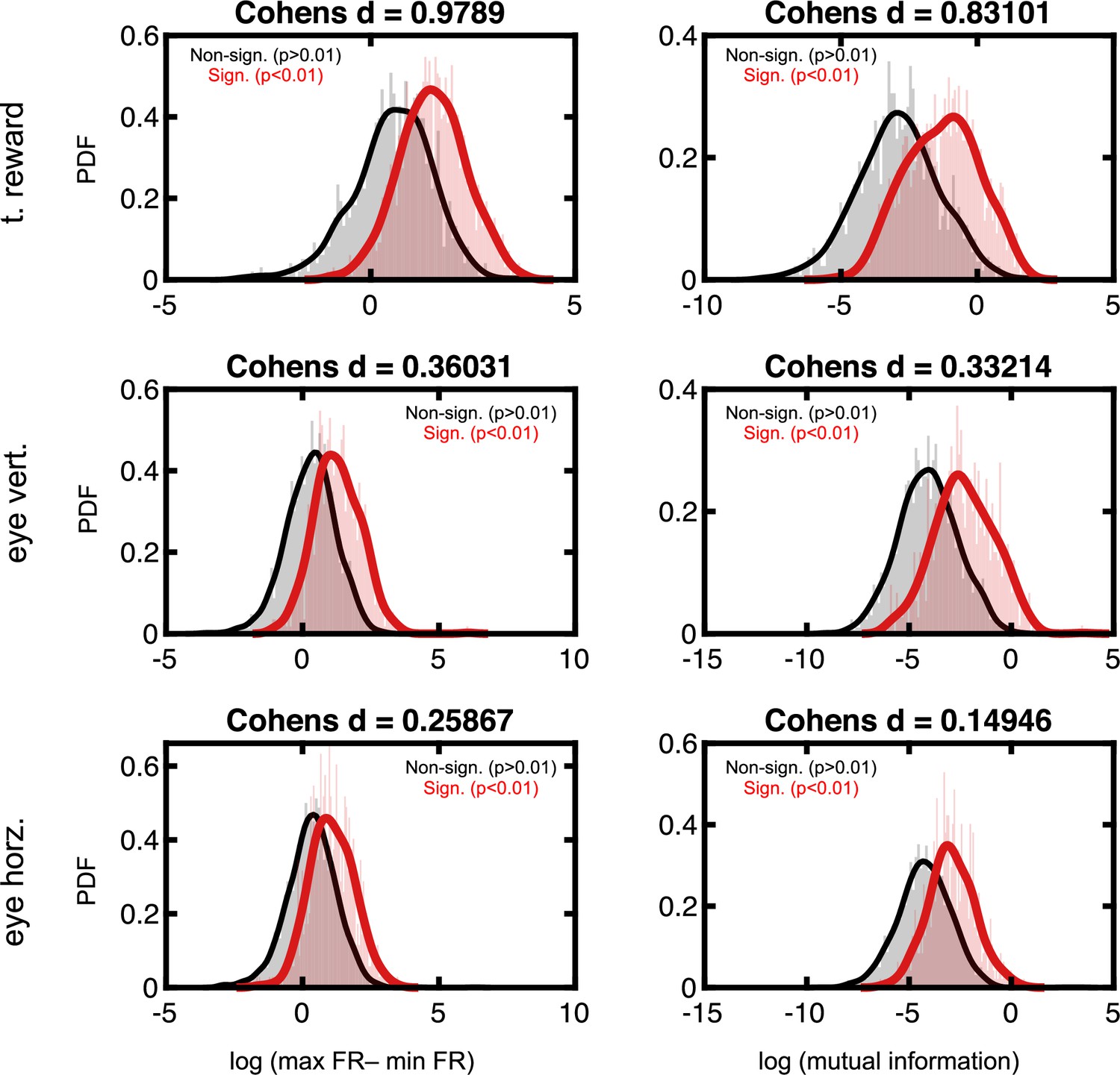
Effect sizes in the firing rate space for neurons deemed to code for reward and eye position.
Format follows that of Figure 2—figure supplement 3.
Figure 2—figure supplement 7
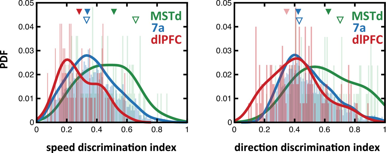
Speed and direction discrimination index for neurons in dorsomedial superior temporal area (MSTd), 7a, and dorsolateral prefrontal cortex (dlPFC).
To allow for direct comparison with prior studies, we compute the discrimination index (see Methods) for speed (i.e., linear velocity) and direction (i.e., angular velocity) in MSTd (green), 7a (blue), and dlPFC (red). Full triangles at the top indicate the mean of each population recorded from here (in their corresponding color), while the empty blue triangles show the mean in Avila et al., 2019 (7a recording) and the empty green triangles show the mean in Chen et al., 2008 (MSTd recordings).
Figure 2—figure supplement 8
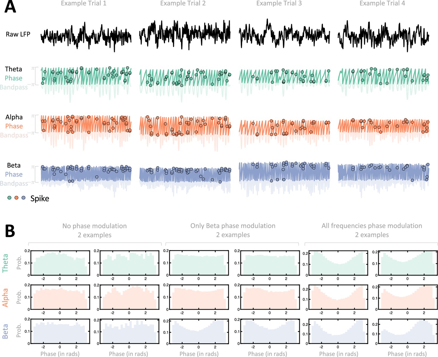
Illustration of spike-local field potential (LFP) phase locking.
(A) Example trials. For each of four example trials (different sessions as well) we show the raw LFP (top), as well as the band-passed version (transparent) and extracted phase (opaque) in theta (green, second row), alpha (orange, third row), and beta (blue, fourth row) ranges. Spikes are represented by dots, and they are placed on the y-axis according to the phase of the ongoing LFP. That is, across rows spikes occur at the same time along the x-axis, but are at different y-locations. If a neuron is phased-locked to LPF in a given range, spikes should predominantly occur at the same y location (as is seen in these examples for the beta band). (B) Example sessions. For six example neurons, we show the distribution of phases (x-axis, in radians) at which spikes occurred, throughout the entire session. We show two example neurons that were not modulated by LFP phase (first and second column), two example neurons that were modulated solely by beta frequency phases (third and fourth column), and finally two example neurons that were modulated by phases at theta, alpha, and beta frequencies.
Figure 2—figure supplement 9
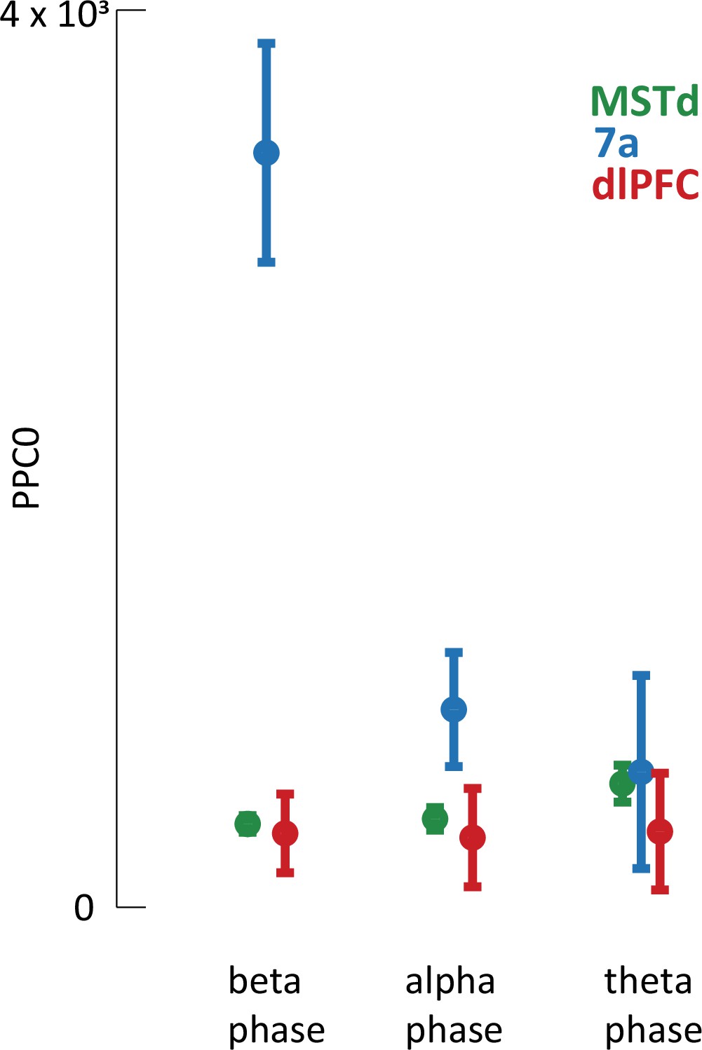
Pairwise phase consistency.
The findings related to spike-local field potential (LFP) phase coupling reported in the main text are based on the Poisson generalized additive model (P-GAM), as are the rest tuning properties reported. However, detecting a correlation between when spikes occur and the phase of LFPs may be biased by a number of factors, for example the firing rate of neurons or the amplitude of LFP oscillations. In turn, we corroborated the spike-LFP phase coupling results by computing the pairwise phase consistency (PPC0), a bias-free estimator (see Vinck et al., 2010, for details). This analysis confirmed the findings from the main text in demonstrating greater spike-LFP phase coupling in area 7a, particularly within the beta and alpha ranges. Mean PPC across all neurons and sessions are reported separately by brain region and frequency range. Error bars are SEM.
Figure 2—figure supplement 10
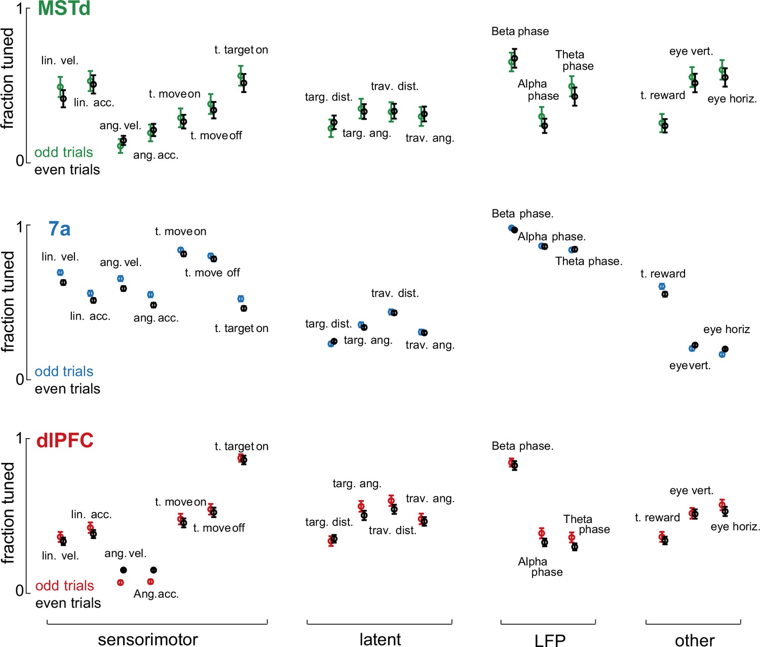
Stability in the fraction of neurons tuned to different task variables.
To test the stability in the Poisson generalized additive model (P-GAMs) estimates, we divided our datasets in even and odd trials. We fitted separate P-GAMs and plot the fraction of neurons tuned (y-axis) to each task variable (x-axis) according to brain area (dorsomedial superior temporal area [MSTd], 7a, and dorsolateral prefrontal cortex [dlPFC]) and whether these were odd or even trials. Error bars are 99% CI. Estimates in the fraction of neurons tuned were very stable.
Figure 2—figure supplement 11
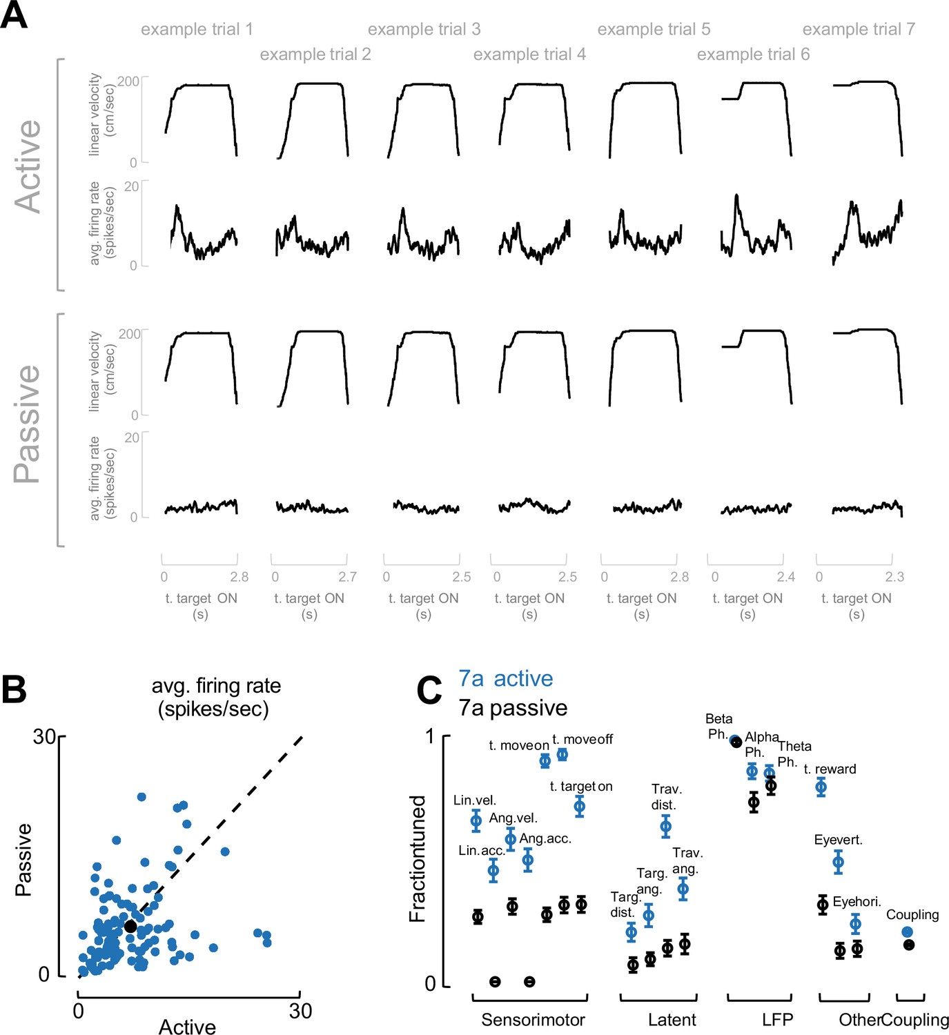
Task engagement drives neural tuning.
(A) Example trials. To demonstrate that the fraction of neurons tuned to different task variables reported in Figure 2F are driven by task engagement and not purely low-level visual input, in a control experiment (two sessions) we recorded from area 7a (117 neurons) as a monkey first actively engaged in the task (top), and then passively viewed replayed the exact visual input (bottom). We show seven example trials, demonstrating that the linear velocity during active and passive trials matched (same for other task variables, not shown). Instead, the population evoked responses (one trial, average across the entire population of simultaneously recorded neurons) was evident during active but not passive trials. (B) Average firing rate. Firing rate (averaged over the entire recording) did not differ between active (x-axis) and passive (y-axis) viewing (blue dots are single cells in 7a, black dot is the mean, dashed black line is identity). (C) Fraction of neurons tuned and coupled. The fraction of neurons tuned to different task variables, and the fraction of neurons coupled to each other in area 7a, were blunted (but not entirely absent) during passive viewing. The exceptions were variables related to internal neural dynamics, notably the phase locking of spiking activity to LFP phase in theta, alpha, and beta band.
Figure 3 with 4 supplements
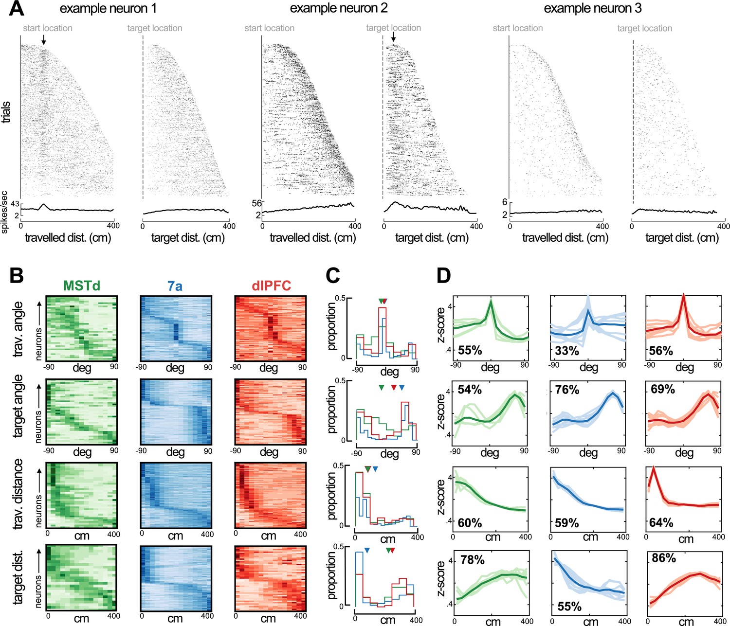
Preferred angle and distance from origin and to target in dorsomedial superior temporal area (MSTd), 7a, and dorsolateral prefrontal cortex (dlPFC).
(A) Rasters and average firing rate of three example neurons, sorted by their maximal distance from origin and to target. The first example neuron (left) responds at a distance of ~100 cm from origin and is not modulated by distance to target. The second example (middle) responds to a close distance to target (~30 cm). Arrows at the top of these rasters indicate the preferred distance from origin (example 1) and to target (example 2). We include a third example (tuned to movement stop) as a control, demonstrating that responding to a distance near the target and to stopping behavior are distinguishable. (B) Heatmaps showing neural responses (y-axis) sorted by preferred angles from origin (top), angle to target (second row), distance from origin (third row), and distance to target (bottom row) for MSTd (green), 7a (blue) and dlPFC (red) in Monkey S (data simultaneously recorded). Darker color indicates higher normalized firing rate. Neurons were sorted based on their preferred distances/angles in even trials and their responses during odd trials is shown (i.e., sorting is cross-validated, see Methods). (C) Histograms showing the probability of observing a given preferred angle or distance across all three monkeys. Inverted triangles at the top of each subplot indicate the median. Of note, however, medians may not appropriately summarize distributions in the case of bimodality. (D) We clustered the kernels driving the response to angle or distance to origin and from the target. Here, we show 10 representatives from each cluster (thin and transparent lines), as well as the mean of the cluster as a whole (ticker line). The inset quantifies the percentage of tunings within a particular area and for the particular variable that were deemed to belong within the cluster depicted (the most frequent one).
Figure 3—figure supplement 1
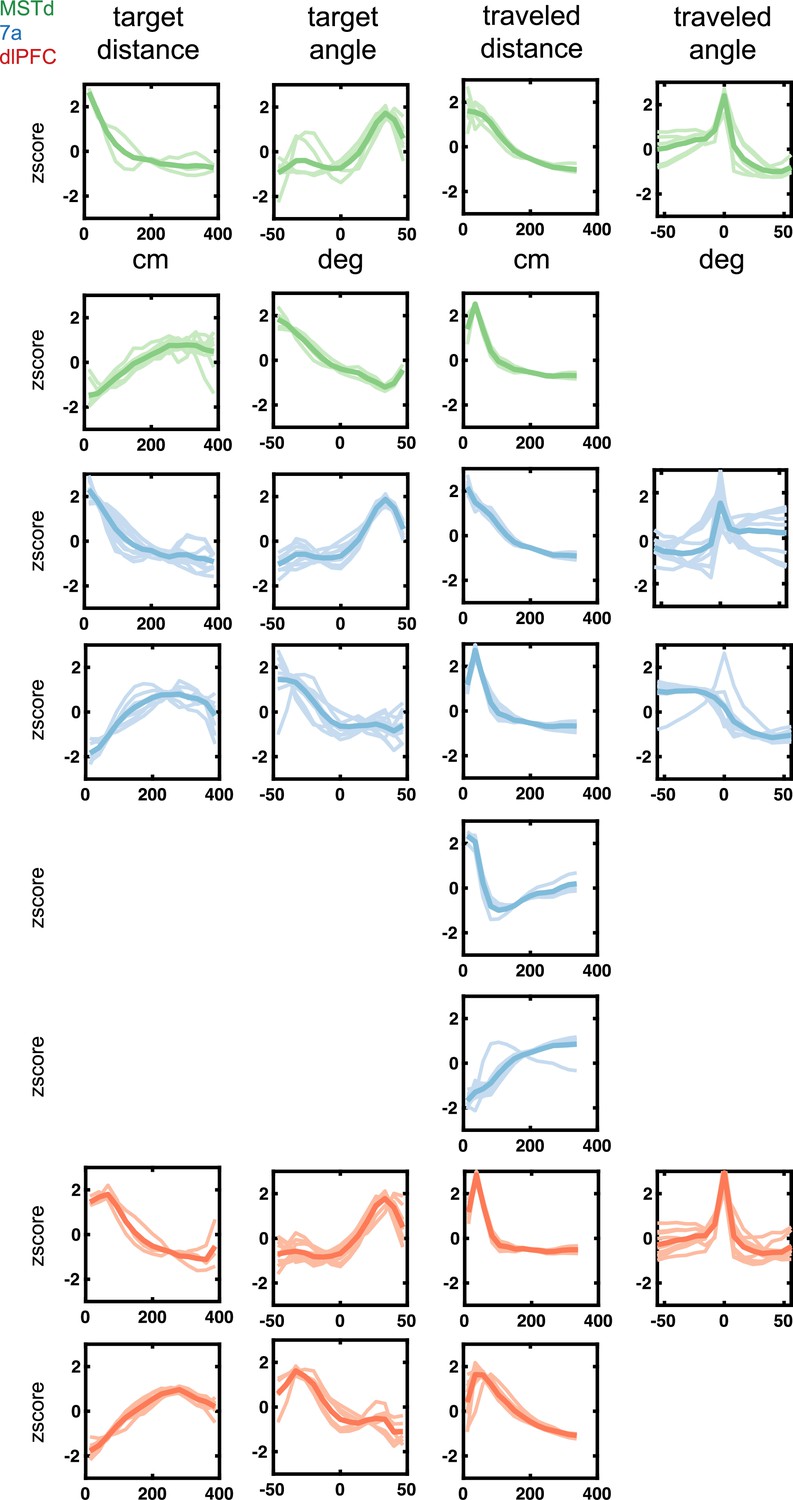
Latent tuning functions (radial and angular distance to target and from origin) encountered in dorsomedial superior temporal area (MSTd) (green), area 7a (blue), and dorsolateral prefrontal cortex (dlPFC) (red).
Tuning function clusters were determined by Density-Based Spatial Clustering of Applications with Noise (DBSCAN). Ten example tuning functions are plotted per cluster (in semi-transparent), as well as the average of all tuning functions within the given cluster type (opaque and thicker line). Y-axis are firing rates (in Hz) z-scored and x-axis spans the state space of the particular variable, in cm for radial distances and degrees for angles (see top row).
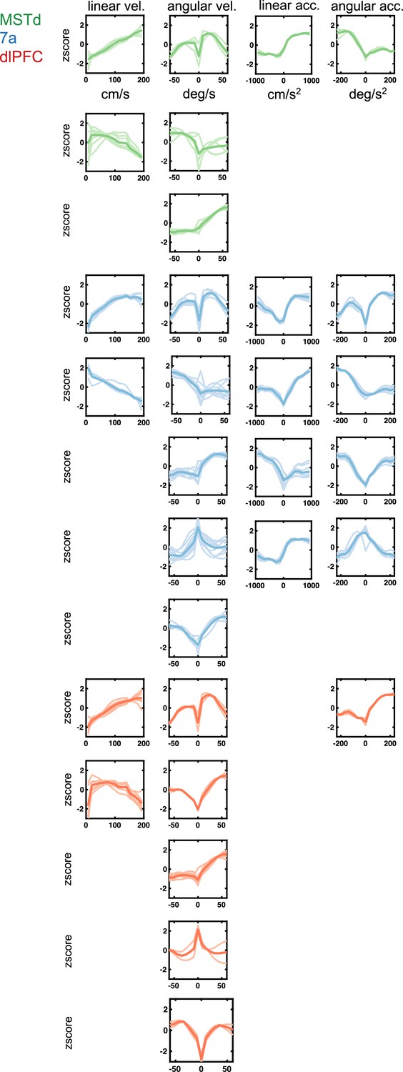
Figure 3—figure supplement 2
Sensorimotor tuning functions to continuous variables (linear and angular velocity and acceleration) encountered in dorsomedial superior temporal area (MSTd) (green), area 7a (blue), and dorsolateral prefrontal cortex (dlPFC) (red).
Tuning function clusters were determined by Density-Based Spatial Clustering of Applications with Noise (DBSCAN). For each cluster, 10 example tuning functions are plotted (semi-transparent and background), as well as the average of all tuning functions within the given cluster type (opaque and thicker line). Y-axis are firing rates (in Hz) z-scored and x-axis spans the state space of the particular variable, in cm/s for linear velocity, deg/s for angular velocity, cm/s2 for linear acceleration, and deg/ s2 for angular acceleration (see top row).
Figure 3—figure supplement 3
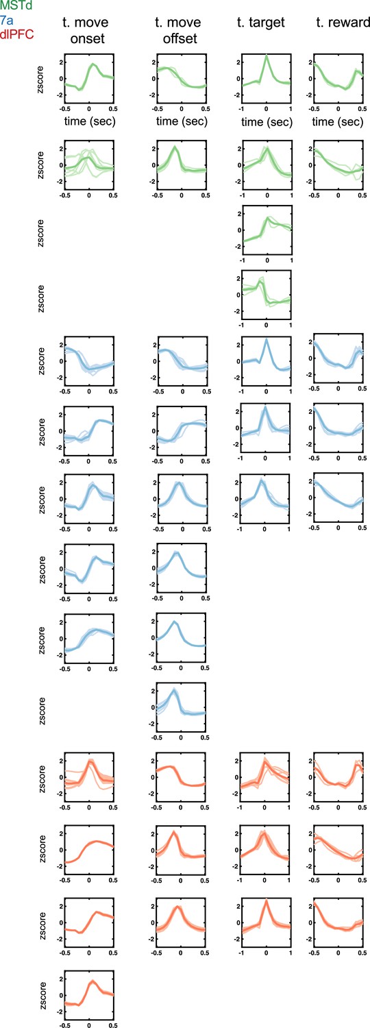
Temporal kernels (time of movement onset and offset, time of target onset and reward presentation) encountered in dorsomedial superior temporal area (MSTd) (green), area 7a (blue), and dorsolateral prefrontal cortex (dlPFC) (red).
Tuning function clusters were determined by Density-Based Spatial Clustering of Applications with Noise (DBSCAN). Ten example tuning functions are plotted per cluster (transparent), as well as the average of all tuning functions within the given cluster type (opaque and thicker line). Y-axis are firing rates (in Hz) z-scored and x-axis is time relative to the discrete event, in seconds (see top row).
Figure 3—figure supplement 4
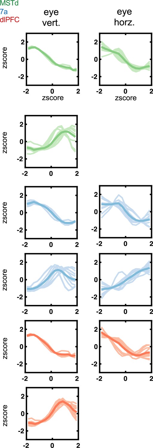
Tuning functions to eye position variables (vertical and horizontal) encountered in dorsomedial superior temporal area (MSTd) (green), area 7a (blue), and dorsolateral prefrontal cortex (dlPFC) (red).
Tuning function clusters were determined by Density-Based Spatial Clustering of Applications with Noise (DBSCAN). Ten example tuning functions are plotted per cluster (semi-transparent), as well as the average of all tuning functions within the given cluster type (opaque and thicker line). Y-axis are firing rates (in Hz) z-scored, and x-axis eye position, also in z-score.
Figure 4 with 4 supplements
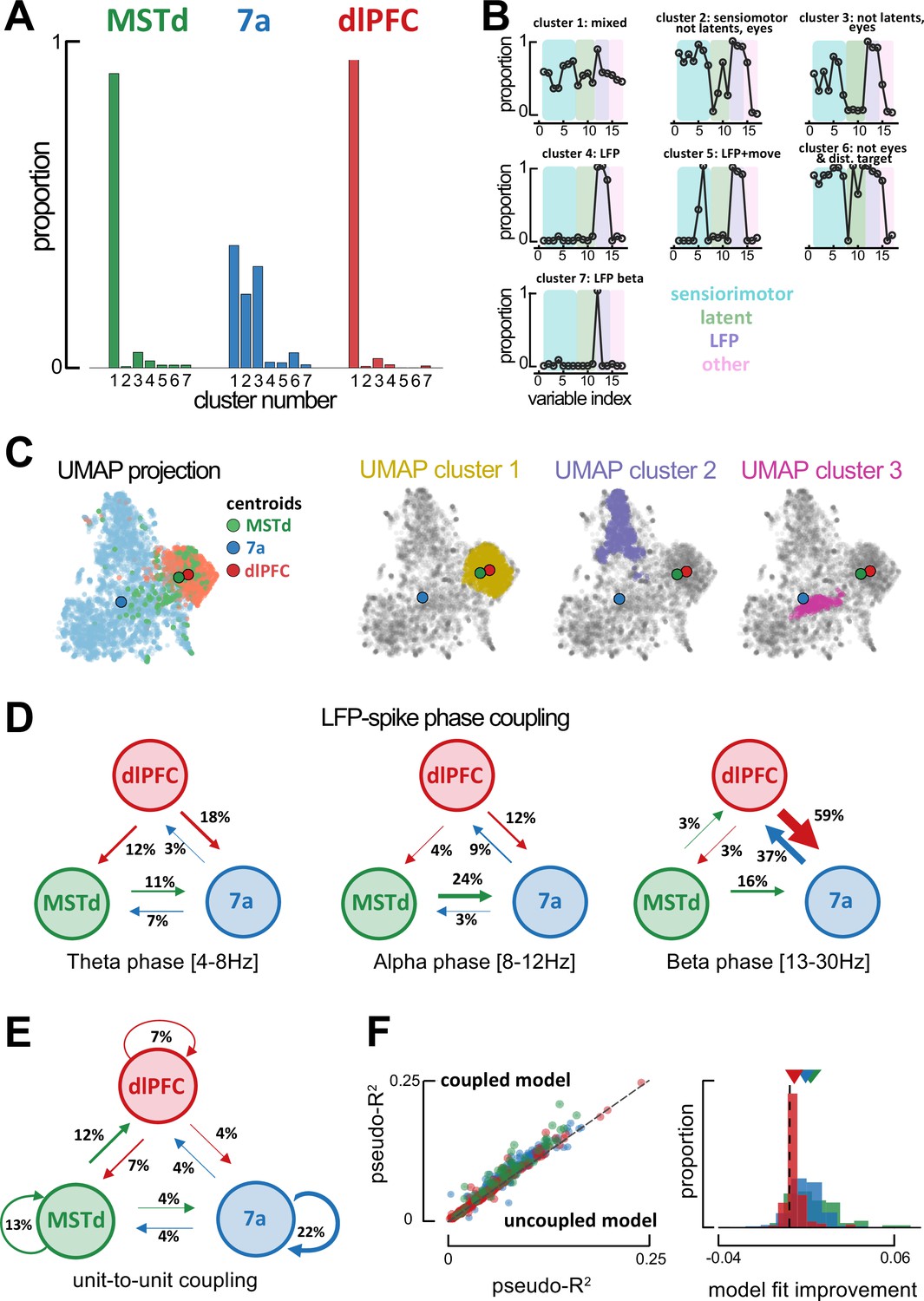
Global single-unit encoding profiles and unit-to-unit coupling properties suggest a common functional role for dorsomedial superior temporal area (MSTd) and dorsolateral prefrontal cortex (dlFPC).
(A) Proportion of neurons being classified into distinct cluster (x-axis, seven total) according to which task parameters they were significantly tuned to. (B) Fraction of neurons tuned to each of the 17 task variables (order is the same as in Figure 2C, E, F) according to cluster. (C) Uniform Manifold Approximation and Projection (UMAP) of the tuning function shapes, color coded by brain area (first column) or Density-Based Spatial Clustering of Applications with Noise (DBSCAN) cluster (second, third, and forth column). (D) Fraction of neurons whose spiking activity is phase-locked to local field potential (LFP) phases in other areas, in theta (leftmost), alpha (center) and beta (rightmost) bands. An arrow projecting from, for example, MSTd to 7a (center, 0.24), indicates that the neuron in area 7a is influenced by ongoing LFP phase in MSTd. Width of arrows and associated number indicate the proportion of neurons showing the particular property. (E) As (D) but for unit-to-unit coupling. An arrow projecting from, for example, MSTd to dlPFC indicates that the firing of a neuron in MSTd will subsequently influence spiking activity in dlPFC. (F) Left: Cross-validated pseudo-R2 of the full encoding model (y-axis) and a reduced model without within and across area unit-to-unit coupling (x-axis). Right: Probability distribution of the change in pseudo-R2 from the reduced to the full model.
Figure 4—figure supplement 1
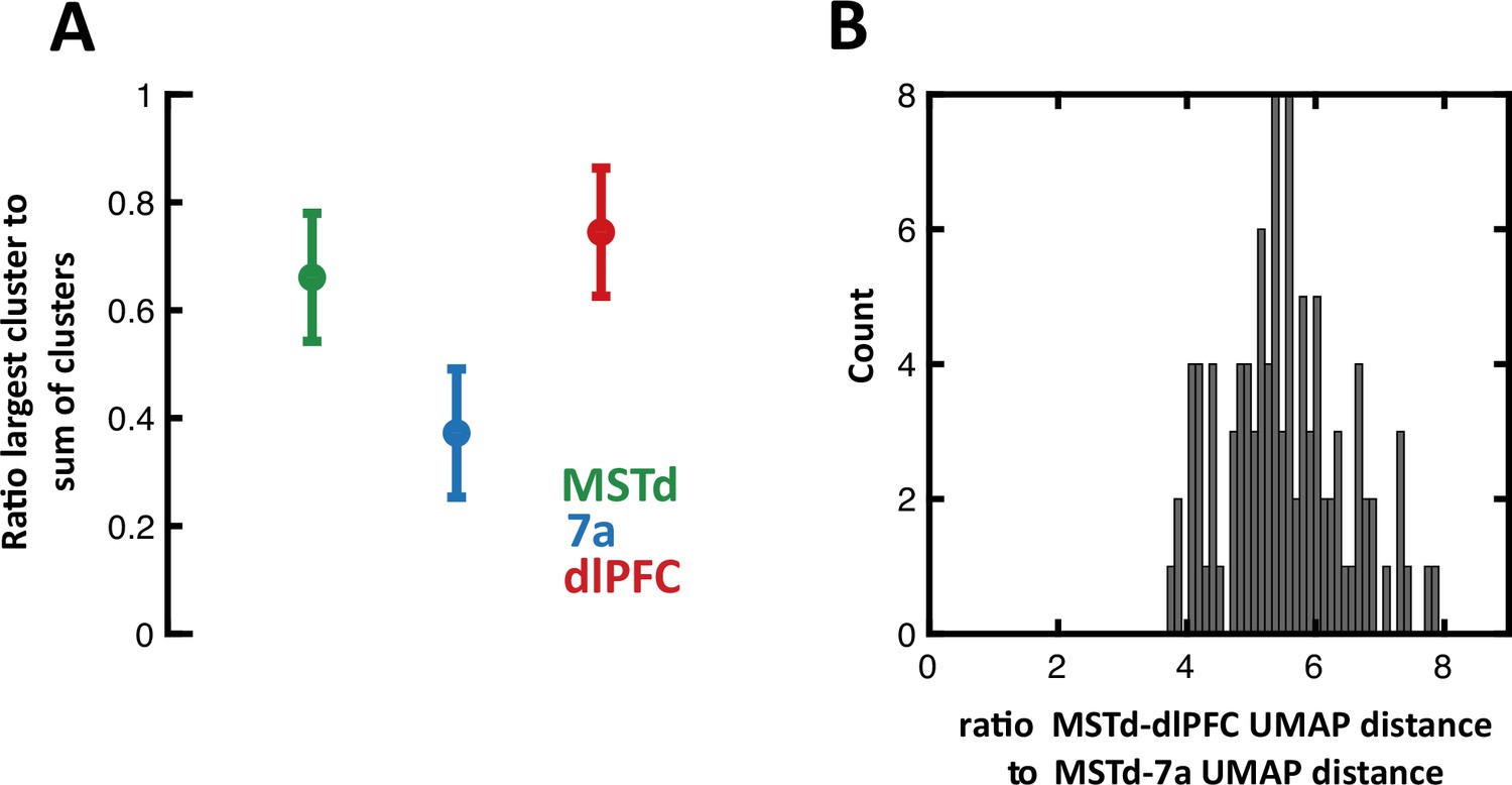
Clustering results, subsampling from neurons in dorsolateral prefrontal cortex (dlPFC) and 7a to match the number of units recorded from in dorsomedial superior temporal area (MSTd).
(A) We performed spectral (Jaccard) clustering of neurons based on their 1×17 vector of Booleans, indicating whether they were tuned or not to particular task variables (Figure 4A). Here, we perform this operation 10,000 times, while randomly selecting (without replacement) 231 neurons from 7a and dlPFC. Thus, the full matrix clustered was 693 (231 × 3 brain areas) × 17 (task variables). Given that on each run clusters are assigned an arbitrary cluster number, for each run we compute the ratio of the largest cluster size to the total number of units per area (231). Namely, in the main text we report that MSTd and dlPFC are predominantly represented by one mixed-selective cluster, while 7a is represented in three approximately equal sized clusters. The results here concord with those in the main text, demonstrating that approximately 70% of neurons in MSTd and dlPFC belong to a single cluster, while approximately 35% of neurons belong to the largest cluster in area 7a. Circles are the mean across 10,000 iteration, error bars are 95% CI. (B) 100 iterations of Uniform Manifold Approximation and Projection (UMAP) while randomly subsampling from 7a and dlPFC to match the number of units in MSTd. On each run, we compute the distance in UMAP space between MSTd and dlPFC, and between MSTd and 7a. Then we compute their ratio (MSTd-to-dlPFC/MSTd-to-7a, thus >1 indicating closer MSTd-to-dlPFC distances). The figure shows the full distribution of ratios, concurring with the main text that MSTd and dlPFC are approximately six times closer in UMAP space, than MSTd and 7a are.
Figure 4—figure supplement 2
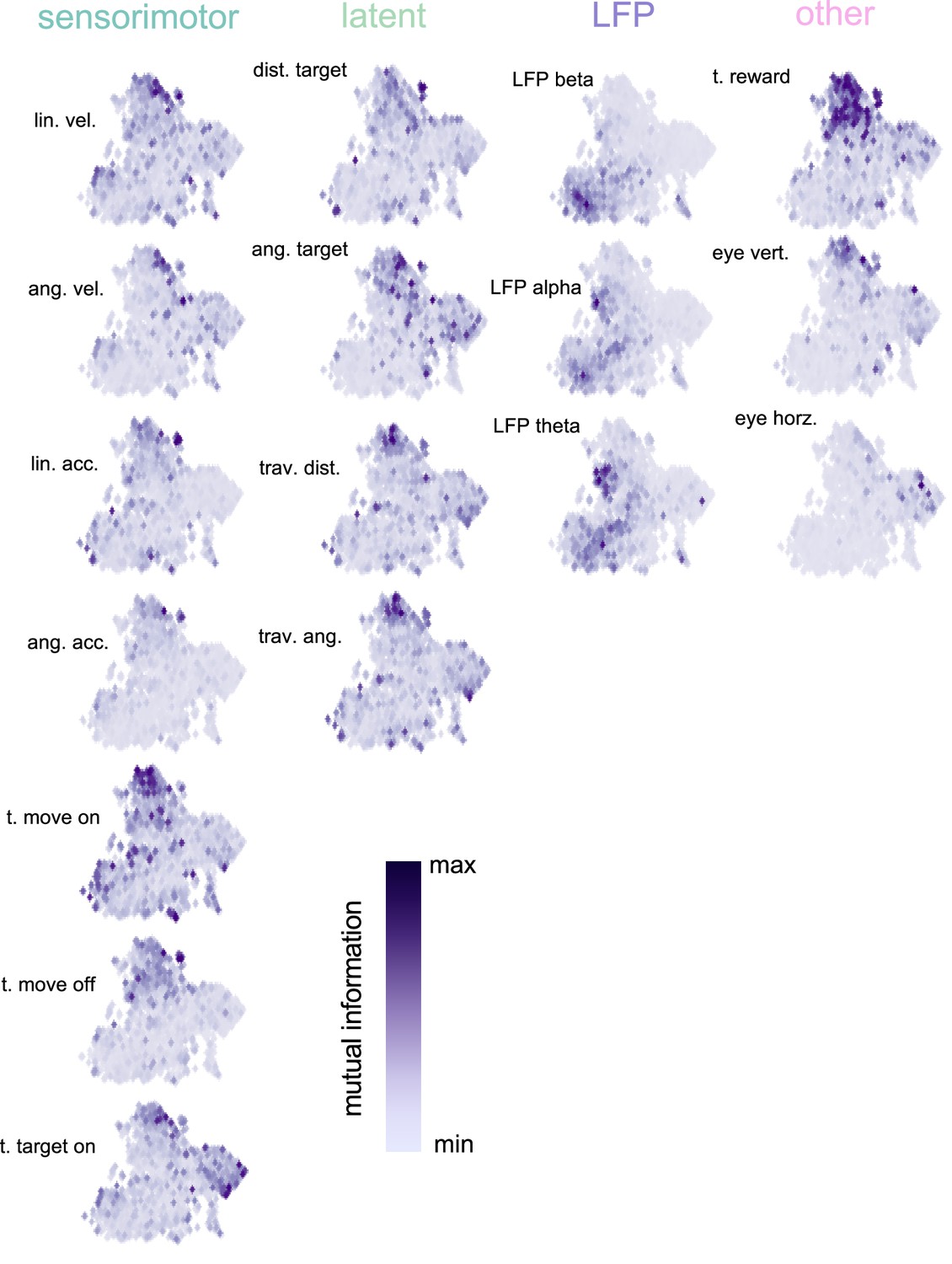
Uniform Manifold Approximation and Projection (UMAP) (McInnes et al., 2020) space color coded by mutual information with each task variable.
Each subplot is normalized between its minimum and maximum mutual information (MI). Results demonstrate that the UMAP finds meaningful clusters – neurons with high MI for a particular variable clustering together – even though the algorithm is not known about task variables or MI. The plots also highlight the distribution in MI for the different variables; for example, most neurons having an intermediary MI for angular acceleration, while a subset of neurons have a very strong MI for the timing of reward.
Figure 4—figure supplement 3
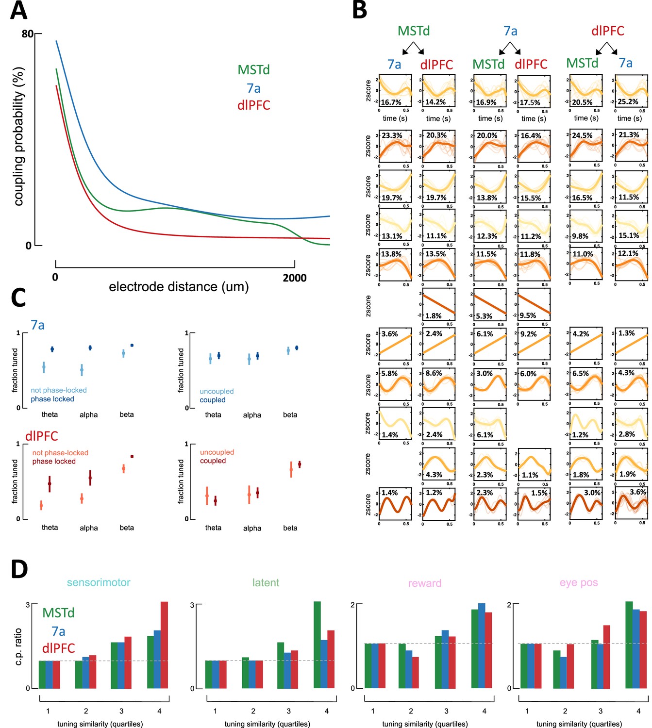
Characteristics of coupling functions within and across areas.
(A) Coupling probability (y-axis) between two neurons as a function of the distance between them (x-axis). This illustration is for data from a single monkey (Monkey S) with recordings in dorsomedial superior temporal area (MSTd) (green, number of coupling pairs = 1714), area 7a (blue, number of coupling pairs = 97,711), and dorsolateral prefrontal cortex (dlPFC) (red, number of coupling pairs = 41,665). As expected, neurons that are closer to each other are more likely to be coupled. Given this effect and that multiple recording techniques were used (with different spacing between electrodes, 400µm in Utah array and 100µm in linear probes), we used these estimates in correcting for coupling probability for a single distance (500µm). (B) Coupling filters across cortical areas. Coupling functions were clustered by Density-Based Spatial Clustering of Applications with Noise (DBSCAN) and are depictured from each of the possible emitters (top) to each of the possible receivers (bottom). The coupling filters are ordered from top to bottom, according to their maximal occurrence for any pair of emitter and receiver. Ten examples (if available) are plotted in semi-transparent and in the background, and the average across all coupling filters of the particular type are plotted in opaque and with a thicker line. Percentages refer to the percent of coupling filters between an emitter and a receiver that were clustered within the given category. X-axis is a z-score of firing rate (in Hz) and y-axis is time in seconds (maximum = 600 ms). Importantly, these coupling filters are not sinusoidal. (C) Fraction of neurons tuned (y-axis) to the phase of theta-, alpha-, and beta-band local field potentials (LFPs) (x-axis) as a function of brain area (top = 7a, bottom = dlPFC) and whether the unit was phase-locked to LFP in the other area (left column) or coupled to a neuron in the other area (right column). Neurons who were tuned to the LFP in a different area (dark blue) were significantly more likely to be tuned to the LFP in their own area (left column) than neurons that were not tuned to the phase of LFP in another area (light blue). On the other hand, whether units were coupled or not with neurons in another area (uncoupled in light blue and coupled in dark blue) did not impact their likelihood of being tuned to the ongoing phase of LFPs in their own area (right column). MSTd is not depicted, as there was no phase locking of dlPFC neurons to the ongoing LFP phase in MSTd. This analysis is based on 5929 coupling pairs in area 7a (blue) and 4190 coupling pairs in dlPFC (red).(D) Coupling probability (CP) between any two units given their tuning similarity to sensorimotor, latent, or other (reward and eye positions) variables. Tuning similarity is computed as the correlation in tuning functions, then these are discretized by their tuning similarity (r2 = [0–0.25; 0.25–0.5; 0.5–0.75; 0.75–1]) and averaged within each category (e.g., sensorimotor) and tuning similarity bin. CP is expressed as a ratio, normalized to the bin with lowest tuning similarity (leftmost), such that a CP ratio of~3 (e.g., sensorimotor variables in dlPFC) indicates that coupling is three times more likely given high vs. low tuning similarity.
Figure 4—figure supplement 4
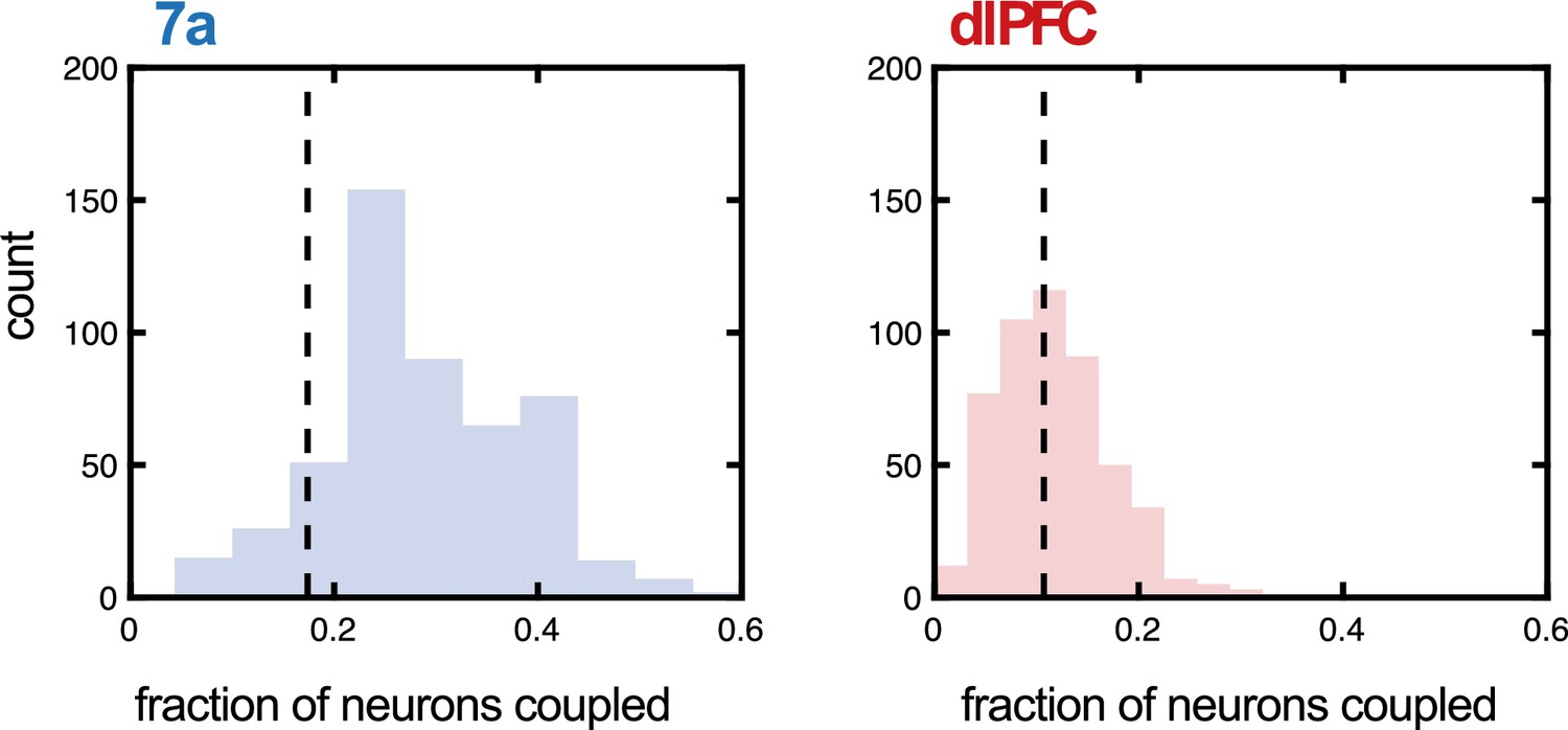
Fraction of neurons coupled in 7a and dorsolateral prefrontal cortex (dlPFC) as a function of probe (Utah array or linear probe).
We questioned whether the type of probe utilized during recording had an impact on the fraction of units the Poisson generalized additive model (P-GAM) estimated as coupled. To address this question, we examined a new set of recordings in 7a (5 sessions, 32 neurons in Monkey B, not reported in the main text), as well as the recordings in dlPFC in Monkey M (55 neurons), both of which were conducted with linear probes. For each area, we computed the fraction of neurons coupled during linear probe recordings, given that the distance between these neurons was 400 µm, the minimal distance between electrodes in the Utah array recordings. Then, we performed 500 iterations where we randomly subsampled from simultaneously recorded neurons in Utah arrays to match the number of simultaneously recorded neurons with the linear probe. We computed the fraction of neurons coupled within this subsample, again only for neurons at a distance of 400 µm. We plot the iterations (from array data) as a histogram (blue for 7a and red for dlPFC), demonstrating that the fraction of neurons tuned did not significantly depend on type of probe used (7a, mean of linear probe = 0.17, 95% CI of array = [0.10 0.49]; dlPFC, mean of linear probe = 0.10, 95% CI of array = [0.03 0.22]).
Figure 5 with 1 supplement
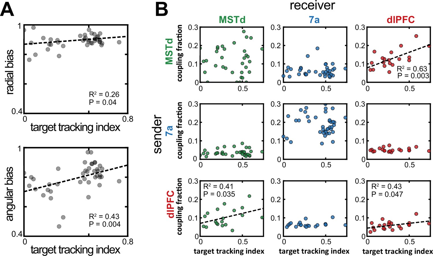
Increased dorsomedial superior temporal area (MSTd)-dorsolateral prefrontal cortex (dlPFC) coupling correlated with an increased likelihood of animals keeping track of the invisible fireflies with their eyes.
(A) Correlation between the target tracking index (x-axis, i.e., tracking the hidden target with their eyes) and the radial (top) or angular (bottom) bias (defined as the slope relating responses and targets, as in Figure 1). Only sessions included in the neural analysis in Panel B were included in Panel A. (B) Correlation between the target tracking index (x-axis) and the fraction of neurons coupled within the ‘sender’ region (y-axis). The diagonal shows within area couplings (MSTd-MSTd, 7a-7a, dlPFC-dlPFC), while off-diagonals show across area couplings. R2 and p-values are shown as insets for the significant correlations.
Figure 5—figure supplement 1
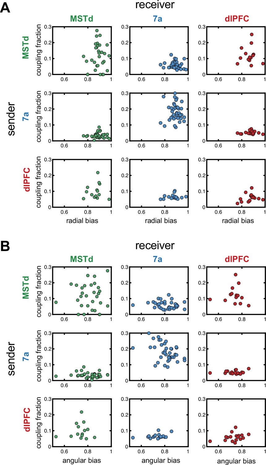
Correlations between fraction of neurons coupled in a ‘sender’ region and steering behavior.
Correlations between the radial (A) or angular (B) bias within a session (defined as the slope relating responses and targets, as in Figure 1) and the fraction of neurons coupled within and across areas. The diagonals show within area couplings (MSTd-MSTd, 7a-7a, dlPFC-dlPFC), while off-diagonals show across area couplings. There was no correlation between fraction of units coupled and steering behavior.
Additional files
Download links
A two-part list of links to download the article, or parts of the article, in various formats.
Downloads (link to download the article as PDF)
Open citations (links to open the citations from this article in various online reference manager services)
Cite this article (links to download the citations from this article in formats compatible with various reference manager tools)
Coding of latent variables in sensory, parietal, and frontal cortices during closed-loop virtual navigation
eLife 11:e80280.
https://doi.org/10.7554/eLife.80280


