Neural learning rules for generating flexible predictions and computing the successor representation
- Zuckerman Institute, Department of Neuroscience, Columbia University, United States
- Basis Research Institute, United States
Figures
Figure 1

The successor representation and an analogous recurrent network model.
(A) The behavior of an animal running down a linear track can be described as a transition between discrete states where the states encode spatial location. (B) By counting the transitions between different states, the behavior of an animal can be summarized in a transition probability matrix . (C) The successor representation matrix is defined as . Here, is shown for . Dashed boxes indicate the slices of shown in (D) and (E). (D) The fourth row of the matrix describes the activity of each state-encoding neuron when the animal is at the fourth state. (E) The fourth column of the matrix describes the place field of the neuron encoding the fourth state. (F) Recurrent network model of the SR (RNN-S). The current state of the animal is one-hot encoded by a layer of input neurons. Inputs connect one-to-one onto RNN neurons with synaptic connectivity matrix . The activity of the RNN neurons are represented by . SR activity is read out from one-to-one connections from the RNN neurons to the output neurons. The example here shows inputs and outputs when the animal is at state 4. (G) Feedforward neural network model of the SR (FF-TD). The matrix is encoded in the weights from the input neurons to the output layer neurons, where the SR activity is read out. (H) Diagram of the terms used for the RNN-S learning rule. Terms in red are used for potentiation while terms in blue are used for normalization (Equation 4). (I) As in (H) but for the feedforward-TD model (Equation 11). To reduce the notation indicating time steps, we use in place of and no added notation for .
Figure 2 with 1 supplement
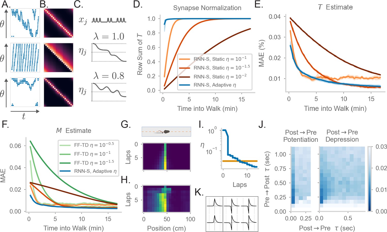
Comparing the effects of an adaptive learning rate and plasticity kernels in RNN-S.
(A) Sample one-minute segments from random walks on a 1 meter circular track. Possible actions in this 1D walk are to move forward, stay in one place, or move backward. Action probabilities are uniform (top), biased to move forward (middle), or biased to stay in one place (bottom). (B) matrices estimated by the RNN-S model in the full random walks from (A).(C) The proposed learning rate normalization. The learning rate for synapses out of neuron changes as a function of its activity and recency bias . Dotted lines are at . (D) The mean row sum of over time computed by the RNN-S with an adaptive learning rate (blue) or the RNN-S with static learning rates (orange). Darker lines indicate larger static learning rates. Lines show the average over 5 simulations from walks with a forward bias, and shading shows 95% confidence interval. A correctly normalized matrix should have a row sum of 1.0. (E) As in (D), but for the mean absolute error in estimating . (F) As in (E), but for mean absolute error in estimating the real , and with performance of FF-TD included, with darker lines indicating slower learning rates for FF-TD. (G) Lap-based activity map of a neuron from RNN-S with static learning rate . The neuron encodes the state at 45cm on a circular track. The simulated agent is moving according to forward-biased transition statistics. (H) As in (G), but for RNN-S with adaptive learning rate. (I) The learning rate over time for the neuron in (G) (orange) and the neuron in (H) (blue). (J) Mean-squared error (MSE) at the end of meta-learning for different plasticity kernels. The pre→post (K+) and post→pre (K-) sides of each kernel were modeled by . Heatmap indices indicate the values s were fixed to. Here, K+ is always a positive function (i.e., was positive), because performance was uniformly poor when K+ was negative. K- could be either positive (left, “Post → Pre Potentiation") or negative (right, “Post → Pre Depression"). Regions where the learned value for was negligibly small were set to high errors. Errors are max-clipped at 0.03 for visualization purposes. 40 initializations were used for each K+ and K- pairing, and the heatmap shows the minimum error acheived over all intializations. (K) Plasticity kernels chosen from the areas of lowest error in the grid search from (J). Left is post → pre potentiation. Right is post → pre depression. Kernels are normalized by the maximum, and dotted lines are at one second intervals.
Figure 2—figure supplement 1
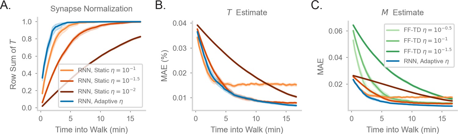
Comparing model performance in different random walks.
(a-c) As in Figure 2D–F of the main document, but for a walk with uniform action probabilities.
Figure 3 with 1 supplement
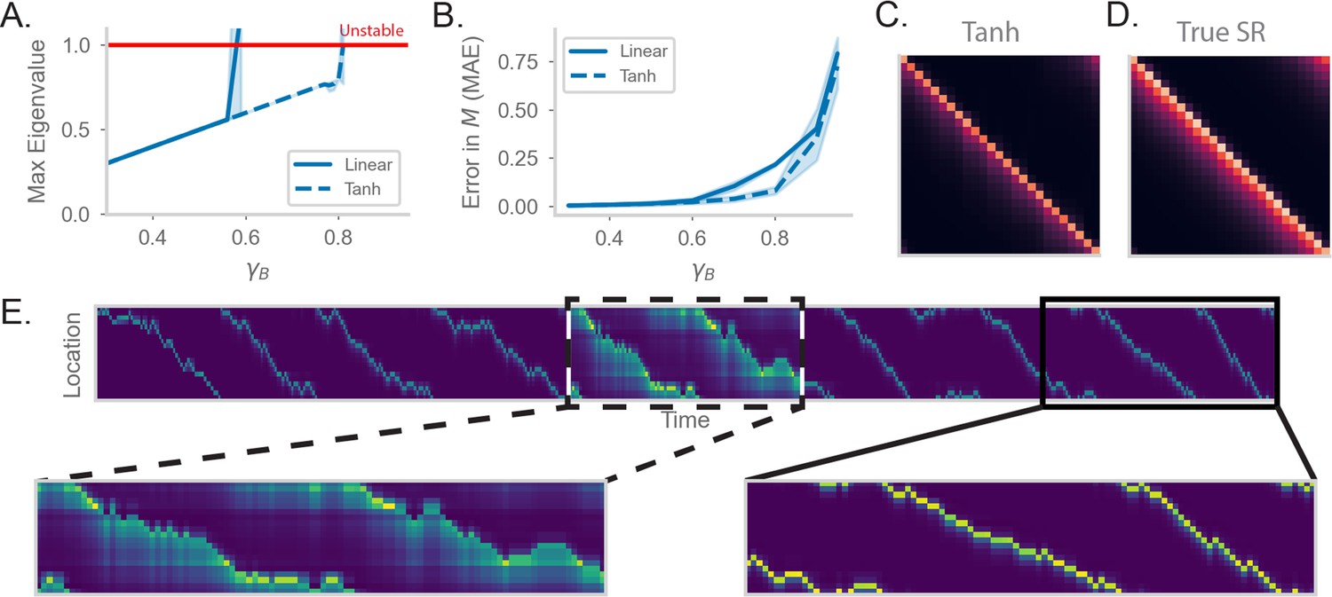
RNN-S requires a stable choice of during learning, and can compute SR with any (A) Maximum real eigenvalue of the matrix at the end of random walks under different .
The network dynamics were either fully linear (solid) or had a tanh nonlinearity (dashed). Red line indicates the transition into an unstable regime. 45 simulations were run for each , line indicates mean, and shading shows 95% confidence interval. (B) MAE of matrices learned by RNN-S with different . RNN-S was simulated with linear dynamics (solid line) or with a tanh nonlinearity added to the recurrent dynamics (dashed line). Test datasets used various biases in action probability selection. (C) matrix learned by RNN-S with tanh nonlinearity added in the recurrent dynamics. A forward-biased walk on a circular track was simulated, and . (D) The true matrix of the walk used to generate (C). (E) Simulated population activity over the first ten laps in a circular track with . Dashed box indicates the retrieval phase, where learning is turned off and . Boxes are zoomed in on three minute windows.
Figure 3—figure supplement 1
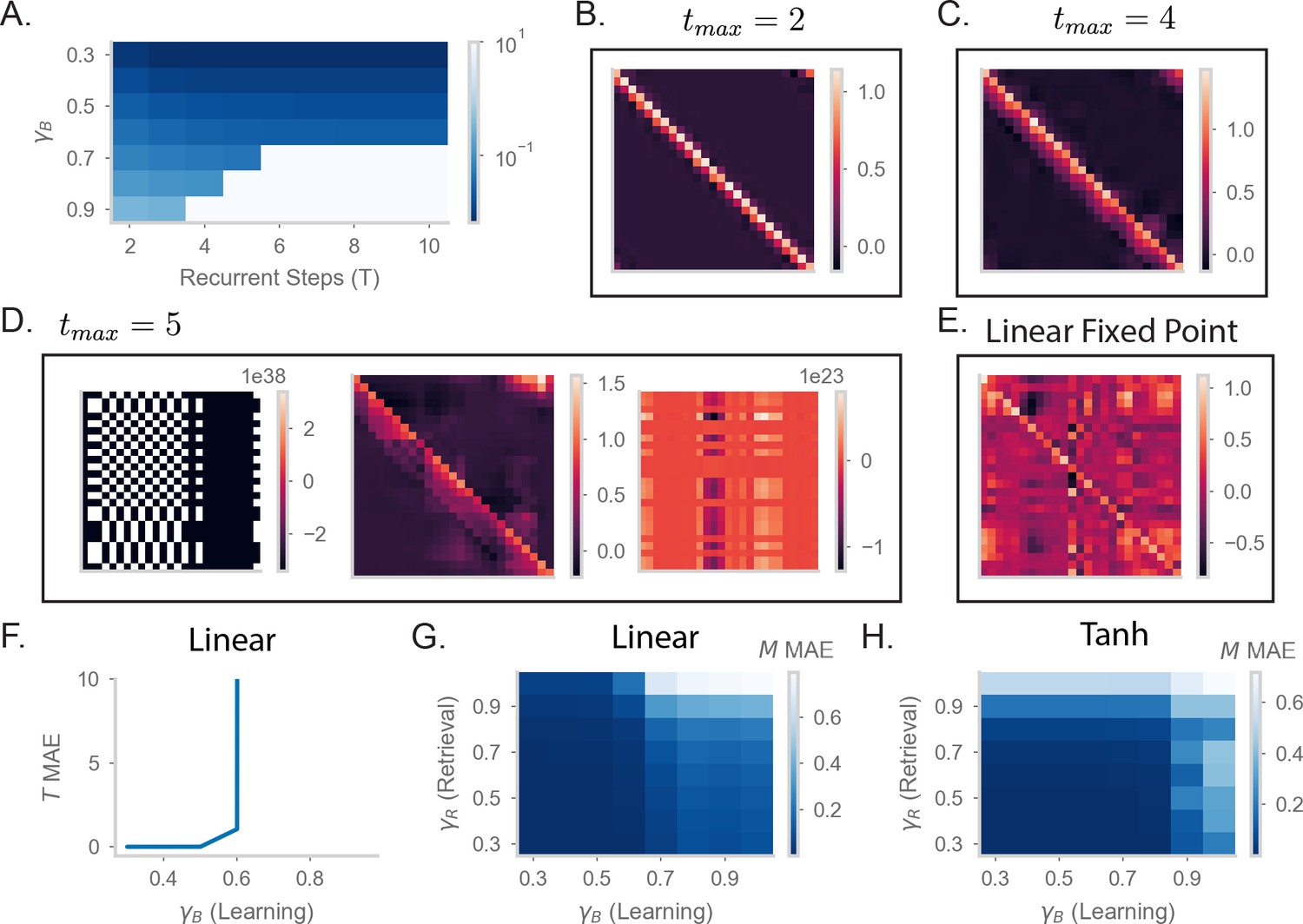
Understanding the effects of recurrency on stability.
(A) Mean absolute error (MAE) of matrices learned by RNN-S with different baseline and different numbers of recurrent steps in dynamics. Test datasets used various biases in action probability selection. Errors are max-clipped at 101 for visualization purposes. (B) matrix learned by RNN-S with two recurrent steps in dynamics and baseline . A forward-biased walk on a circular track was simulated. (C) As in (B), but for four recurrent steps. (D) As in (B), but for five recurrent steps. Three examples are shown from different sampled walks to highlight the runaway activity of the network. (E) As in (B) but for the RNN-S activity calculated as . Note that this calculation amounts to an unstable fixed point in the dynamics that cannot be reached when the network is in an unstable regime. (F) Mean absolute error (MAE) in made by RNN-S with linear dynamics using during learning. (G) MAE in for made by RNN-S with linear dynamics using during learning. (H) As in (G), but the dynamics now have a tanh nonlinearity.
Figure 4 with 1 supplement
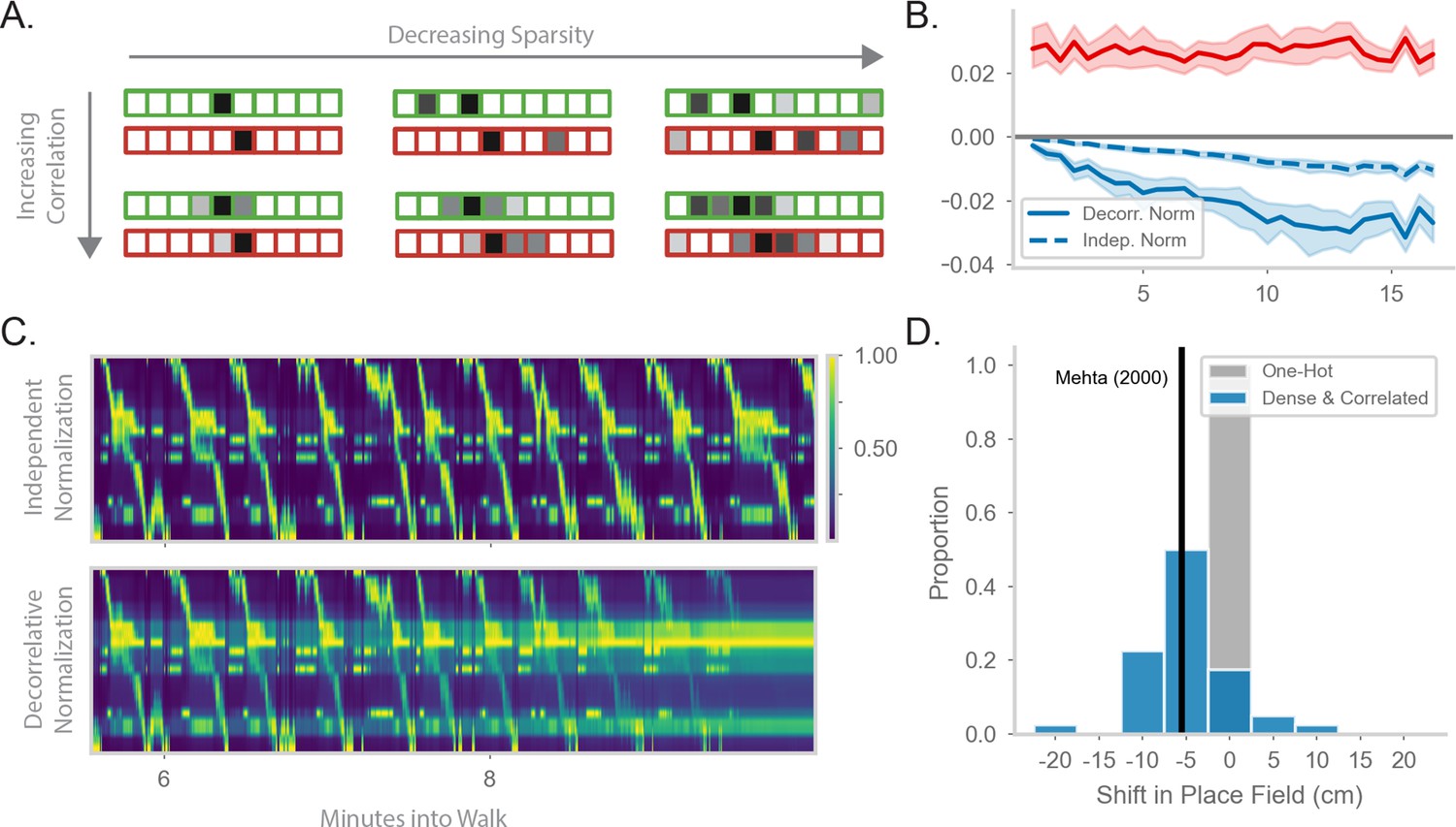
Generalizing the model to more realistic inputs.
(A) Illustration of possible feature encodings for two spatially adjacent states in green and red. Feature encodings may vary in sparsity level and spatial correlation. (B) Average value of the STDP component (red) and the decorrelative normalization (solid blue) component of the gradient update over the course of a random walk. In dashed blue is a simpler Oja-like independent normalization update for comparison. Twenty-five simulations of forward-biased walks on a circular track were run, and shading shows 95% confidence interval. Input features are 3% sparse, with 10 cm spatial correlation. (C) Top: Example population activity of neurons in the RNN-S using the full decorrelative normalization rule over a 2min window of a forward-biased random walk. Population activity is normalized by the maximum firing rate. Bottom: As above, but for RNN-S using the simplified normalization update. (D) Shifts in place field peaks after a half hour simulation from the first two minutes of a 1D walk. Proportion of shifts in RNN-S with one-hot inputs shown in gray. Proportion of shifts in RNN-S with feature encodings (10% sparsity, 7.5 cm spatial correlation, ) shown in blue. Each data point is the average shift observed in one simulated walk, and each histogram is over 40 simulated walks. Solid line indicates the reported measure from Mehta et al., 2000.
Figure 4—figure supplement 1
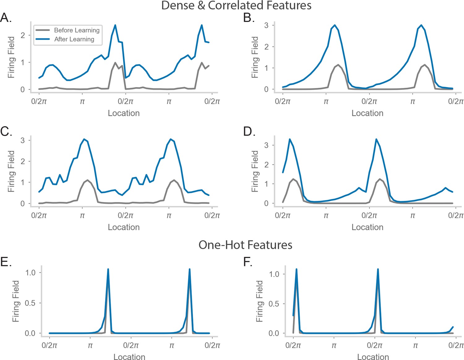
Comparing place field shift and skew effects for different feature encodings.
(A–D) Average firing rate as a function of position on a circular track for four example neurons. The walk and feature encodings were generated as in Figure 4D of the main text. Each neuron is sampled from a different walk. ‘Before Learning’ refers to firing fields made from the first 2-minute window of the walk. ‘After Learning’ refers to firing fields made from the entire walk. (E–F) As in (A–D), but for two neurons from a walk where the features were one-hot encoded.
Figure 5 with 1 supplement
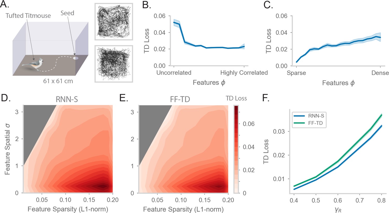
Fitting successor features to data with RNN-S over a variety of feature encodings.
(A) We use behavioral data from Payne et al, where a Tufted Titmouse randomly forages in a 2D environment while electrophysiological data is collected (replicated with permission from authors). Two example trajectories are shown on the right. (B) Temporal difference (TD) loss versus the spatial correlation of the input dataset, aggregated over all sparsity levels. Here, . Line shows mean, and shading shows 95% confidence interval. (C) As in (B), but measuring TD loss versus the sparsity level of the input dataset, aggregated over all spatial correlation levels. (D) TD loss for RNN-S with datasets with different spatial correlations and sparsities. Gray areas were not represented in the input dataset due to the feature generation process. Here, , and three simulations were run for each spatial correlation and sparsity pairing under each chosen . (E) As in (G), but for FF-TD. (F) TD loss of each model as a function of , aggregated over all input encodings. Line shows mean, and shading shows 95% confidence interval.
Figure 5—figure supplement 1
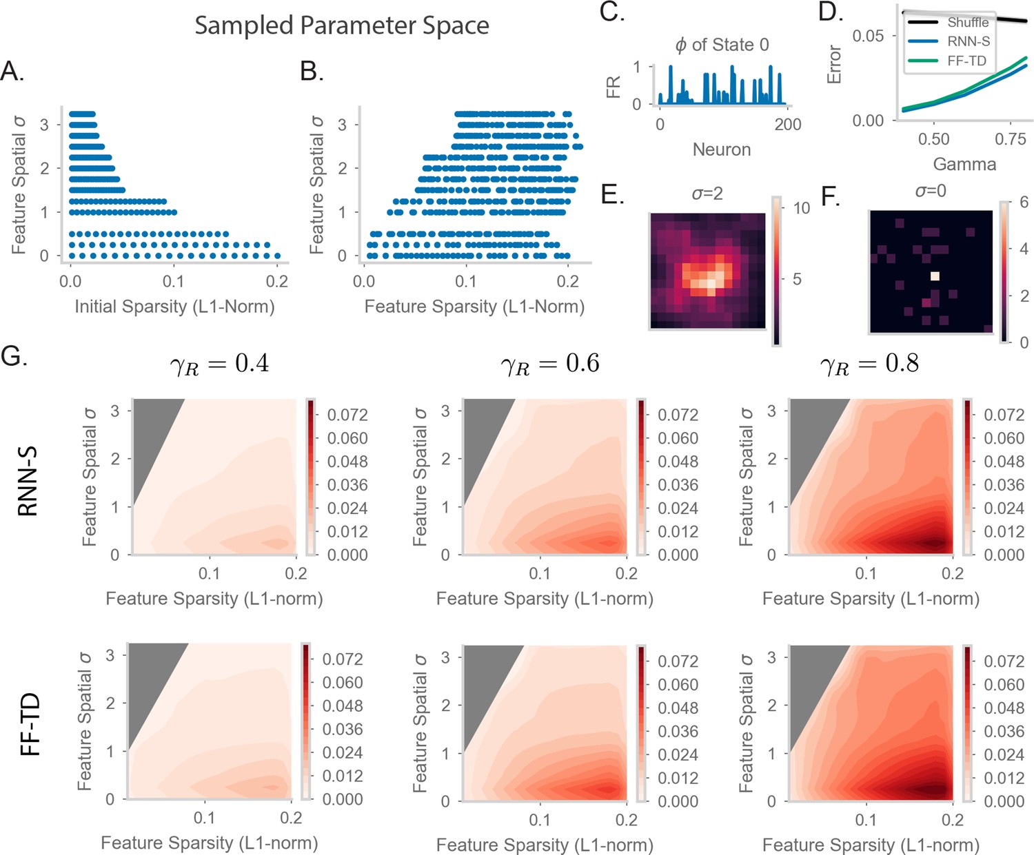
Parameter sweep details and extended TD error plots.
(A) The values of P (initial sparsity of random vectors before spatial smoothing) and σ sampled in our parameter sweep for Figures 5 and 6 in the main text. See methods 4.10 for more details of how feature encodings were generated. (B) The values of S (final sparsity of features, measured after spatial smoothing) and σ sampled in our parameter sweep for Figures 5 and 6 in the main text. (C) A sample state encoded by the firing rate of 200 input neurons. Here, and . (D) As in Figure 5F of the main text, with the results from a random feedforward network included (“Shuffle”). The random network was constructed by randomly drawing weights from the distribution of weights learned by the FF-TD network. The random network is representative of a model without learned structure but with a similar magnitude of weights as the FF-TD model. (E) Spatial correlation of the feature encoding for an example state with the features of all other states. The states are laid out in their position in the 2D arena. Here, the sample state is the state in the center of the 2D arena and . (F) As in (E), but for . (G) As in Figure 5D of the main text, but for RNN-S (first row) and FF-TD (second row) with (left column), (middle column), and (right column).
Figure 6 with 1 supplement
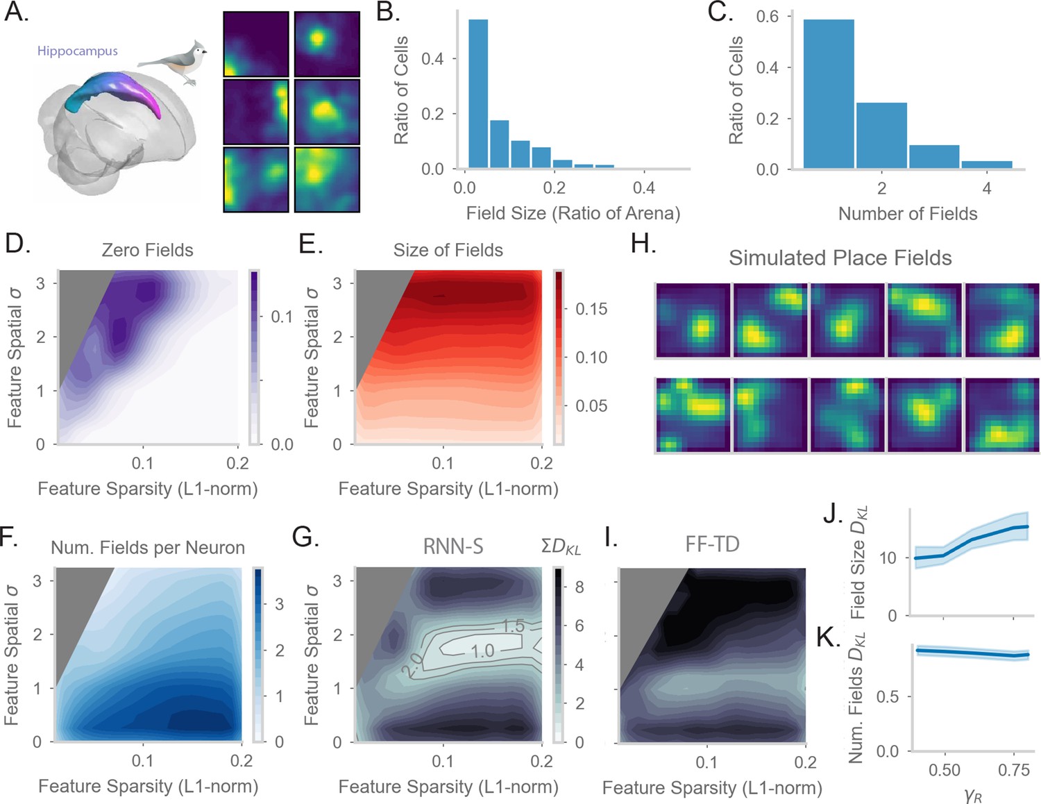
Comparing place fields from RNN-S to data.
(A) Dataset is from Payne et al, where a Tufted Titmouse randomly forages in a 2D environment while electrophysiological data is collected (replicated with permission from authors). (B) Distribution of place cells with some number of fields, aggregated over all cells recorded in all birds. (C) Distribution of place cells with some field size as a ratio of the size of the arena, aggregated over all cells recorded in all birds. (D) Average proportion of non-place cells in RNN-S, aggregated over simulations of randomly drawn trajectories from Payne et al. Feature encodings are varied by spatial correlation and sparsity as in Figure 5. Each simulation used 196 neurons. As before, three simulations were run for each spatial correlation and sparsity pairing under each chosen . (E) As in (D), but for average field size of place cells. (F) As in (D), but for average number of fields per place cell. (G) As in (D) and (E), but comparing place cell statistics using the KL divergence () between RNN-S and data from Payne et al. At each combination of input spatial correlation and sparsity, the distribution of field sizes is compared to the neural data, as is the distribution of number of fields per neuron, then the two values are summed. Contour lines are drawn at values of 1, 1.5, and 2 bits. (H) Place fields of cells chosen from the region of lowest KL divergence. (I) As in (G) but for FF-TD. (J) Change in KL divergence for field size as function of . Line shows mean, and shading shows 95% confidence interval. (K) Same as (J), but for number of fields.
Figure 6—figure supplement 1
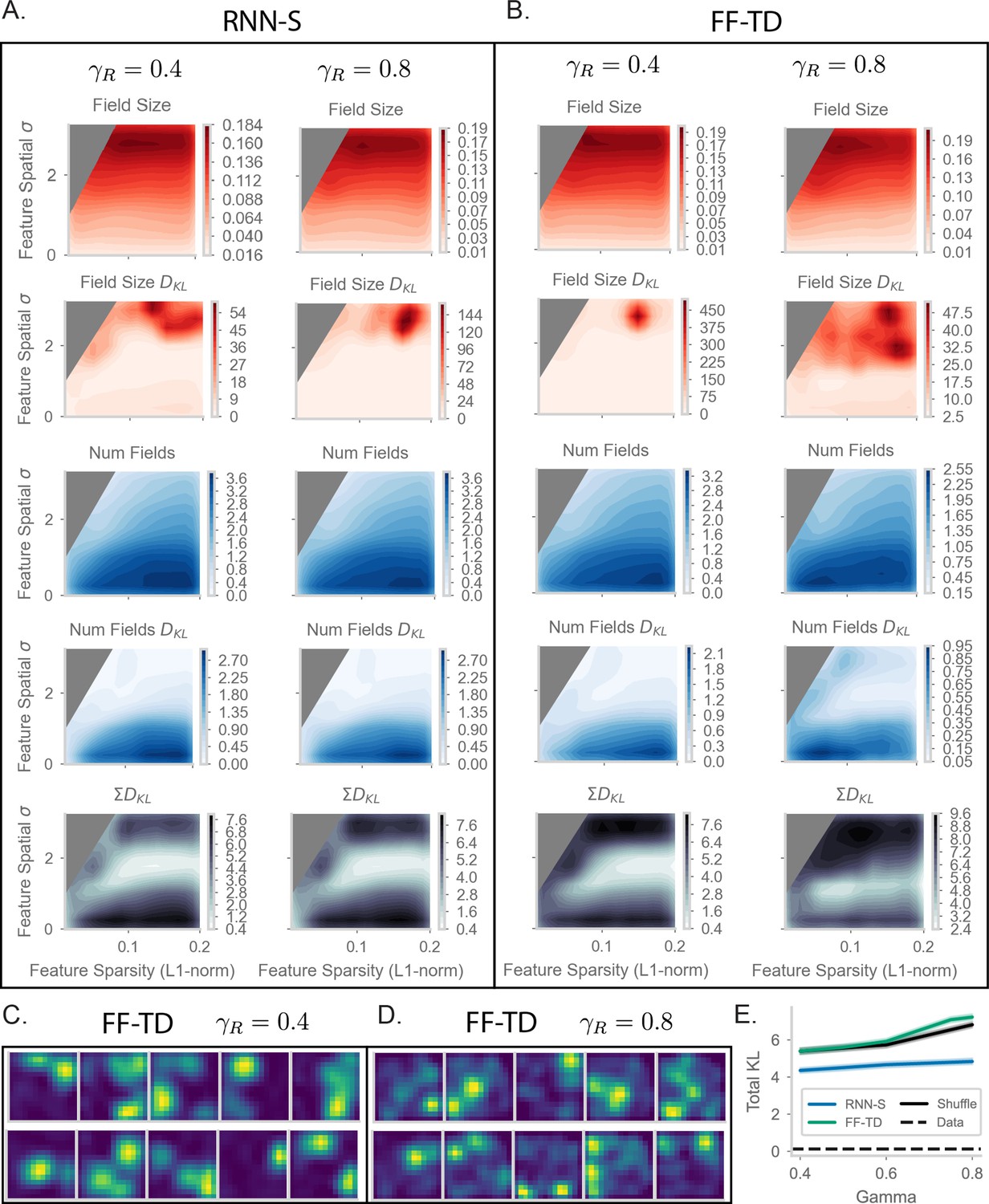
Extended place field evaluation plots.
(A) As in Figure 6E–G of the main text, but for (left column) and (right column). In addition, the plots showing KL divergence (in bits) for the distribution of field sizes and number of fields per cell are shown. (B) As in (A) but for FF-TD. (C) A in Figure 6H of the main text, but for FF-TD with and (D) FF-TD with . (E) Total KL divergence across for RNN-S, FF-TD, the random network from Figure 6D (‘Shuffle’), and the split-half noise floor from the Payne et al. dataset (‘Data’). This noise floor is calculated by comparing the place field statistics of a random halves of the neurons from Payne et al. We measure the KL divergence between the distributions calculated from each random half. This is repeated 500 times, and it is representative of a lower bound on KL divergence. Intuitively, it should not be possible to fit the data of Payne et al as well as the dataset itself can.
Appendix 7—figure 1
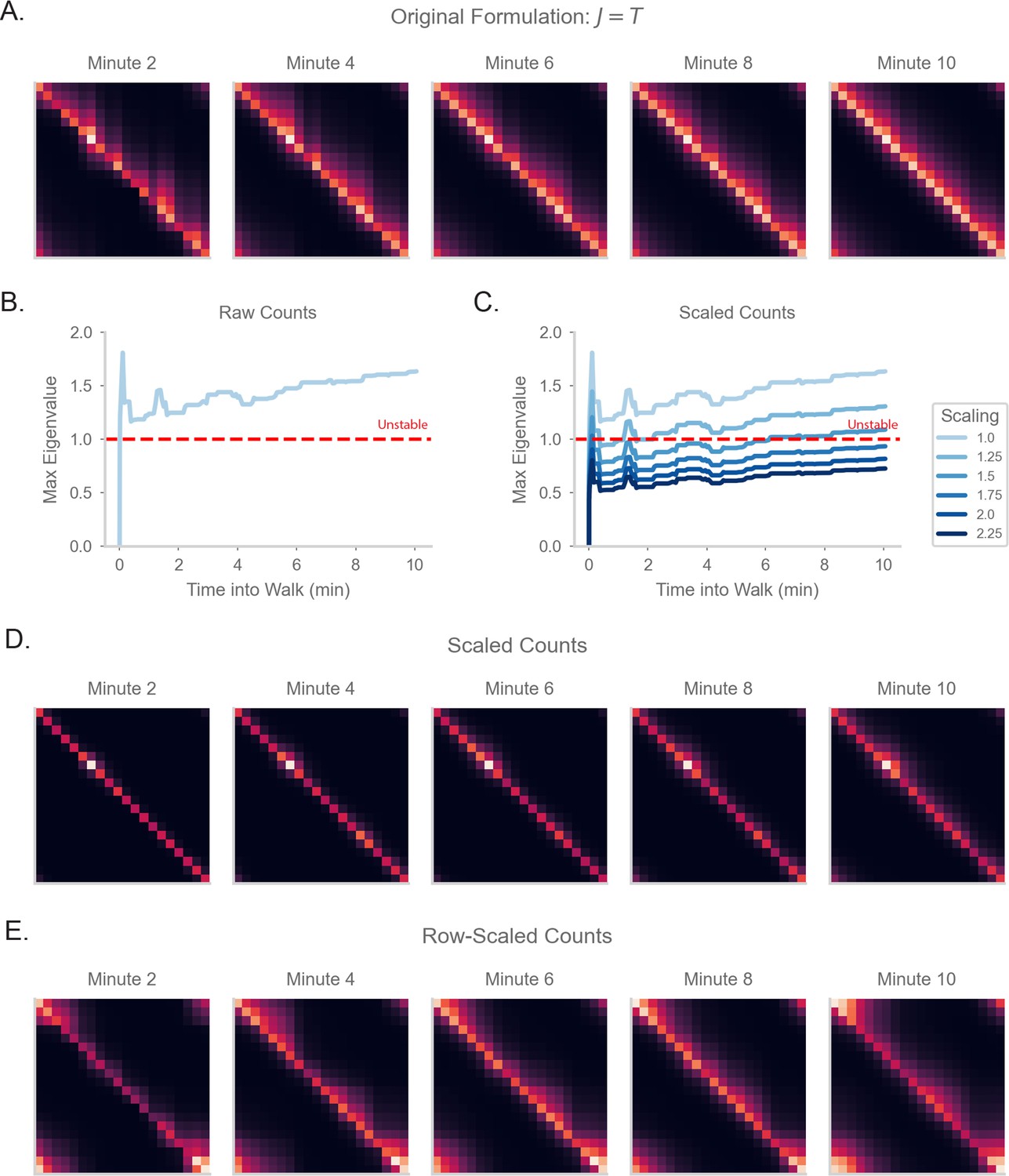
SR matrices under different forms of normalization.
(A) The resulting SR matrix from a random walk on a circular track for 10minutes, if the synaptic weight matrix exactly estimates the transition probability matrix (as in Equation 4). (B) Model as in (A), but with normalization removed. Thus, will be equal to the count of observed transitions, i.e. is equal to the number of experienced transitions from state to state . We will refer to this as a count matrix. The plot show the maximum eigenvalue of the weight matrix, where an eigenvalue indicates instability (Sompolinsky et al., 1988). (C) As in (B), but with an additional scaling factor over the weights of the matrix, such that is multiplied by . (D) Steady state neural activity of the model in (C) with scaling factor 1.75. (E) As in (D), but the count matrix is instead scaled in a row-by-row fashion. Specifically, we divide each row of the count matrix by the maximum of row (and some global scaling factor to ensure stability).
Additional files
Download links
A two-part list of links to download the article, or parts of the article, in various formats.
Downloads (link to download the article as PDF)
Open citations (links to open the citations from this article in various online reference manager services)
Cite this article (links to download the citations from this article in formats compatible with various reference manager tools)
Neural learning rules for generating flexible predictions and computing the successor representation
eLife 12:e80680.
https://doi.org/10.7554/eLife.80680


