Cortical activity during naturalistic music listening reflects short-range predictions based on long-term experience
- Radboud University Nijmegen, Donders Institute for Brain, Cognition and Behaviour, Netherlands
Figures
Figure 1
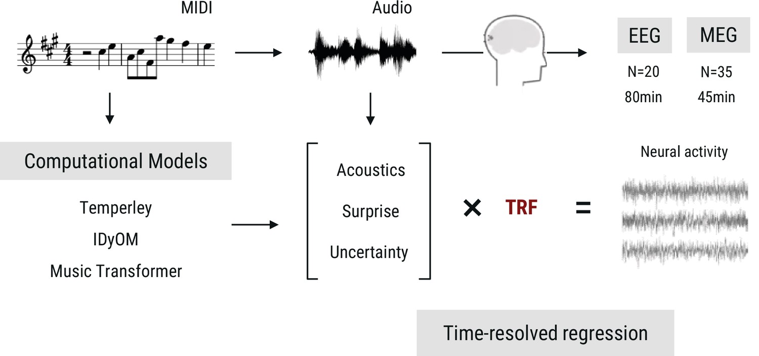
Overview of the research paradigm.
Listeners undergoing EEG (data from Di Liberto et al., 2020) or MEG measurement (novel data acquired for the current study) were presented with naturalistic music synthesized from MIDI files. To model melodic expectations, we calculated note-level surprise and uncertainty estimates via three computational models reflecting different internal models of expectations. We estimated the regression evoked response or temporal response function (TRF) for different features using time-resolved linear regression on the M|EEG data, while controlling for low-level acoustic factors.
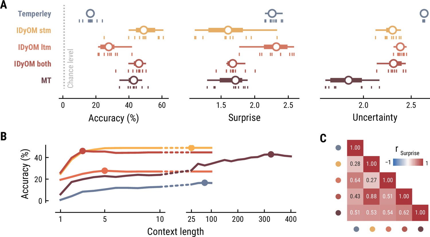
Figure 2
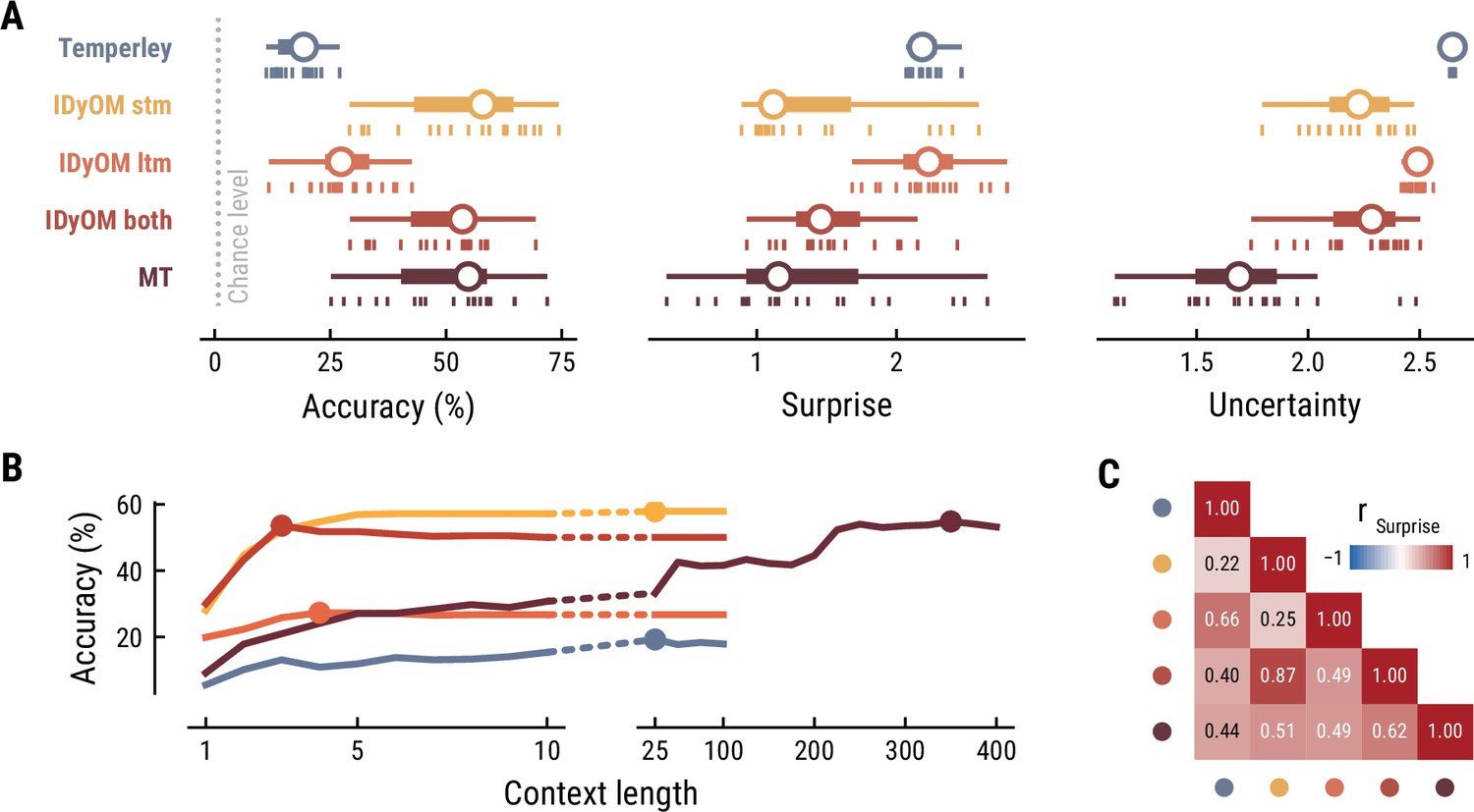
Model performance on the musical stimuli used in the MEG study.
(A) Comparison of music model performance in predicting upcoming note pitch, as composition-level accuracy (left; higher is better), median surprise across notes (middle; lower is better), and median uncertainty across notes (right). Context length for each model is the best performing one across the range shown in (B). Vertical bars: single compositions, circle: median, thick line: quartiles, thin line: quartiles ±1.5 × interquartile range. (B) Accuracy of note pitch predictions (median across 19 compositions) as a function of context length and model class (same color code as (A)). Dots represent maximum for each model class. (C) Correlations between the surprise estimates from the best models. (For similar results for the musical stimuli used in the EEG study, see Appendix 1—figure 2).
Figure 3
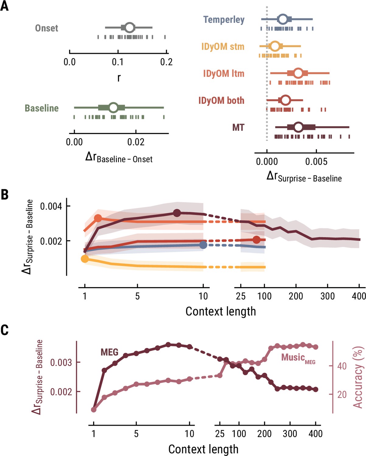
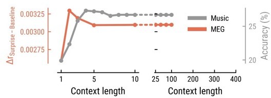
Model performance on MEG data from 35 listeners.
(A) Cross-validated r for the Onset only model (top left). Difference in cross-validated r between the Baseline model including acoustic regressors and the Onset model (bottom left). Difference in cross-validated r between models including surprise estimates from different model classes (color-coded) and the Baseline model (right). Vertical bars: participants; box plot as in Figure 2. (B) Comparison between the best surprise models from each model class as a function of context length. Lines: mean across participants, shaded area: 95% CI. (C) Predictive performance of the Music Transformer (MT) on the MEG data (left y-axis, dark, mean across participants) and the music data from the MEG study (right y-axis, light, median across compositions).
Figure 4
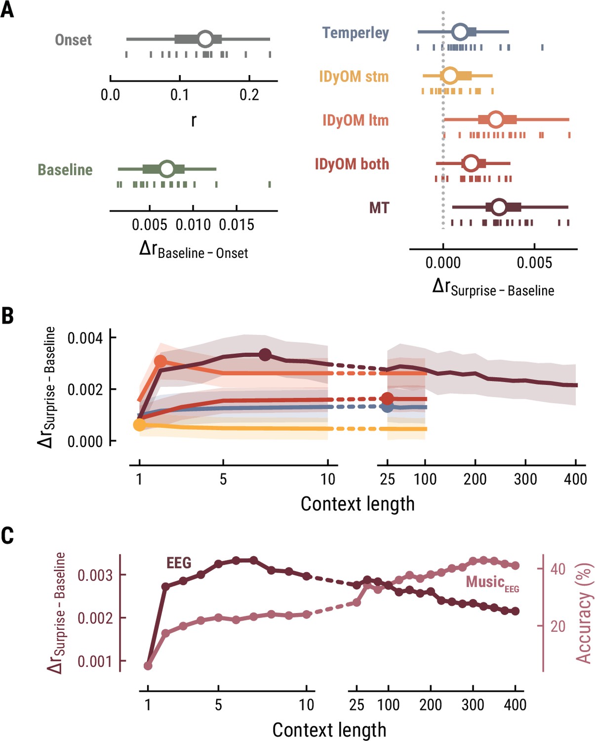
Model performance on EEG data from 20 listeners.
All panels as in Figure 3, but applied to the EEG data and its musical stimuli.
Figure 5
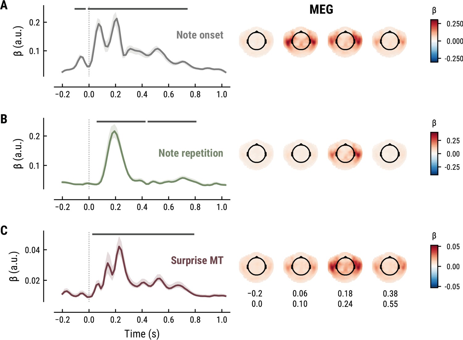
Temporal response functions (TRFs, left column) and spatial topographies at four time periods (right column) for the best model on the MEG data.
(A): Note onset regressor. (B): Note repetition regressor. (C): Surprise regressor from the Music Transformer with a context length of eight notes. TRF plots: Grey horizontal bars: time points at which at least one channel in the ROI was significant. Lines: mean across participants and channels. Shaded area: 95% CI across participants.
Figure 6
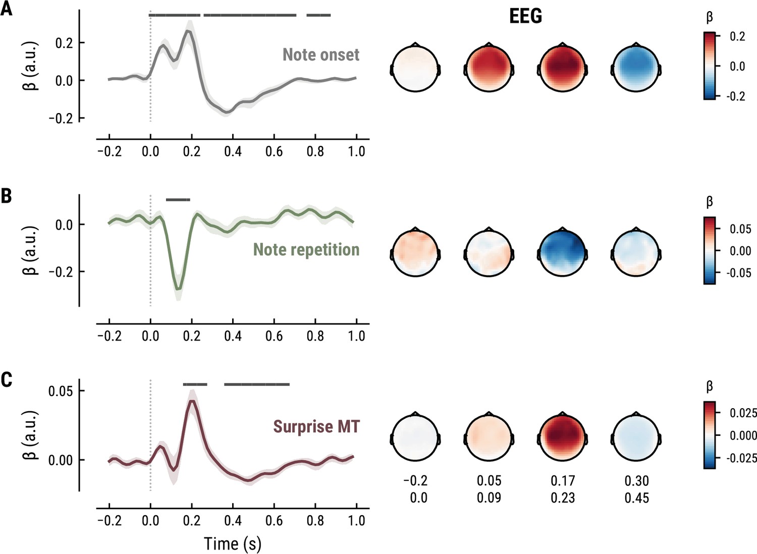
All panels as in Figure 5, but applied to the EEG data and its musical stimuli.
Figure 7
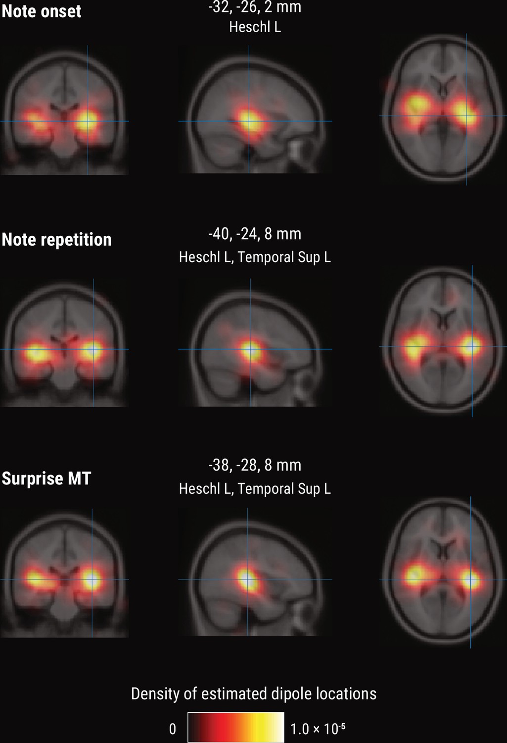
Source-level results for the MEG TRF data.
Volumetric density of estimated dipole locations across participants in the time window of interest identified in Figure 5 (180–240ms), projected on the average Montreal Neurological Institute (MNI) template brain. MNI coordinates are given for the density maxima with anatomical labels from the Automated Anatomical Labeling atlas.
Figure 8
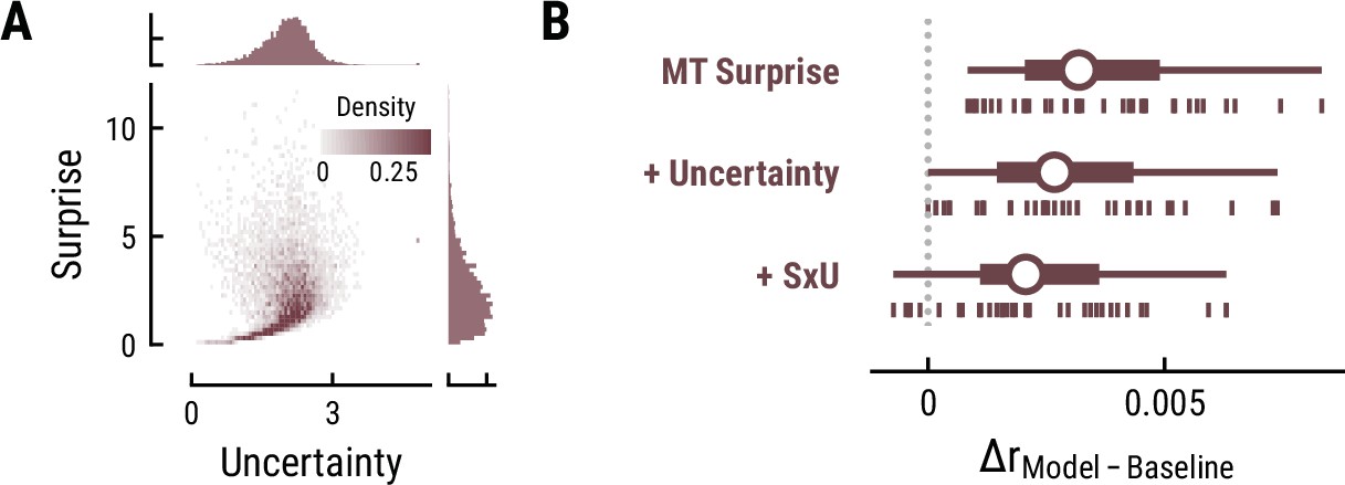
Results for melodic uncertainty.
(A) Relationship between and distribution of surprise and uncertainty estimates from the Music Transformer (context length of eight notes). (B) Cross-validated predictive performance for the Baseline +surprise model (top), and for models with added uncertainty regressor (middle) and the interaction between surprise and uncertainty (SxU, bottom). Adding uncertainty and/or the interaction between surprise and uncertainty (SxU) did not improve but worsen the predictive performance on the MEG data.
Figure 9
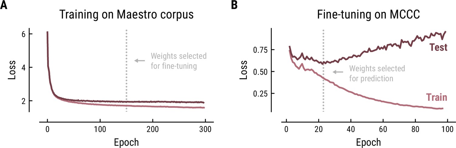
Training (A) and fine-tuning (B) of the Music Transformer on the Maestro corpus and MCCC, respectively.
Cross-entropy loss (average surprise across all notes) on the test (dark) and training (light) data as a function of training epoch.
Appendix 1—figure 1
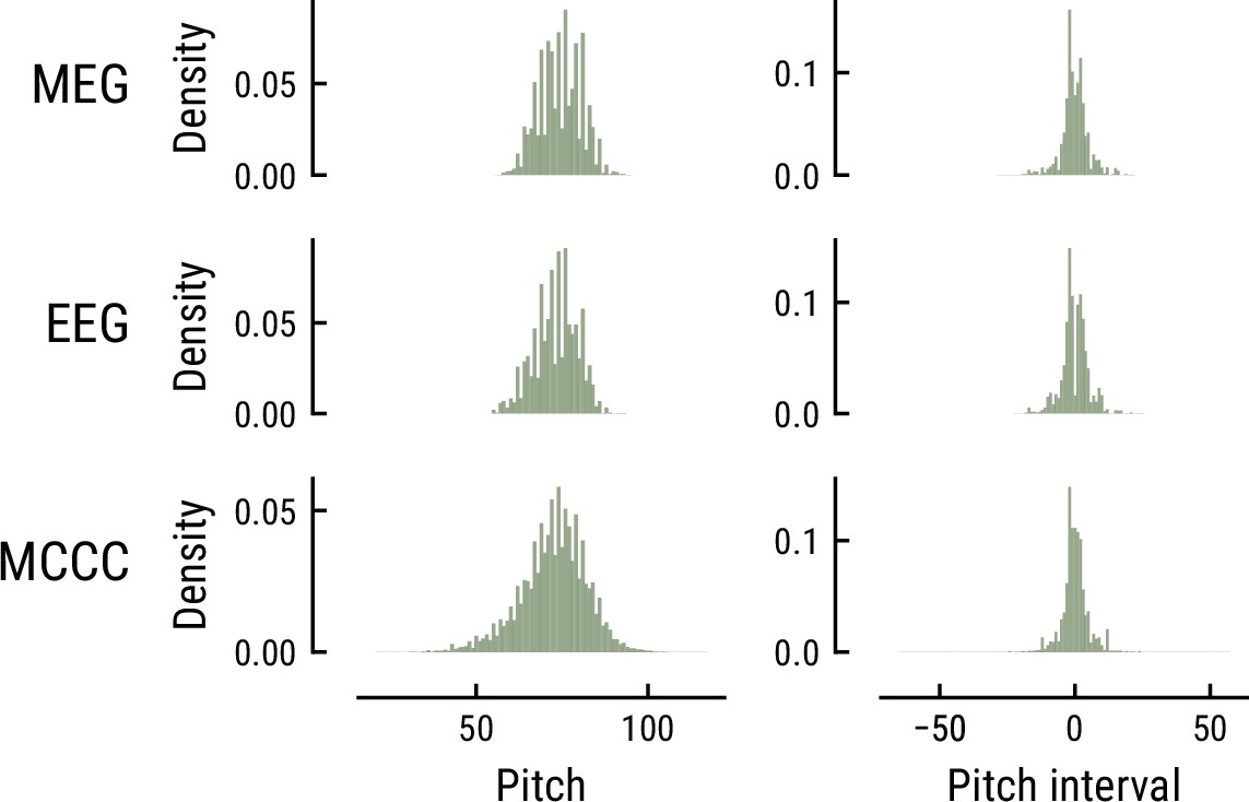
Comparison of the pitch (left) and pitch interval distributions (right) for the music data from the MEG study (top), EEG study (middle), and MCCC corpus (bottom).
Appendix 1—figure 2
Model performance on the musical stimuli used in the EEG study.
(A) Comparison of music model performance in predicting upcoming note pitch, as composition-level accuracy (left; higher is better), median surprise across notes (middle; lower is better), and median uncertainty across notes (right). Context length for each model is the best performing one across the range shown in (B). Vertical bars: single compositions, circle: median, thick line: quartiles, thin line: quartiles ±1.5 × interquartile range. (B) Accuracy of note pitch predictions (median across 10 compositions) as a function of context length and model class (same color code as (A)). Dots represent maximum for each model class. (C) Correlations between the surprise estimates from the best models.
Appendix 1—figure 3
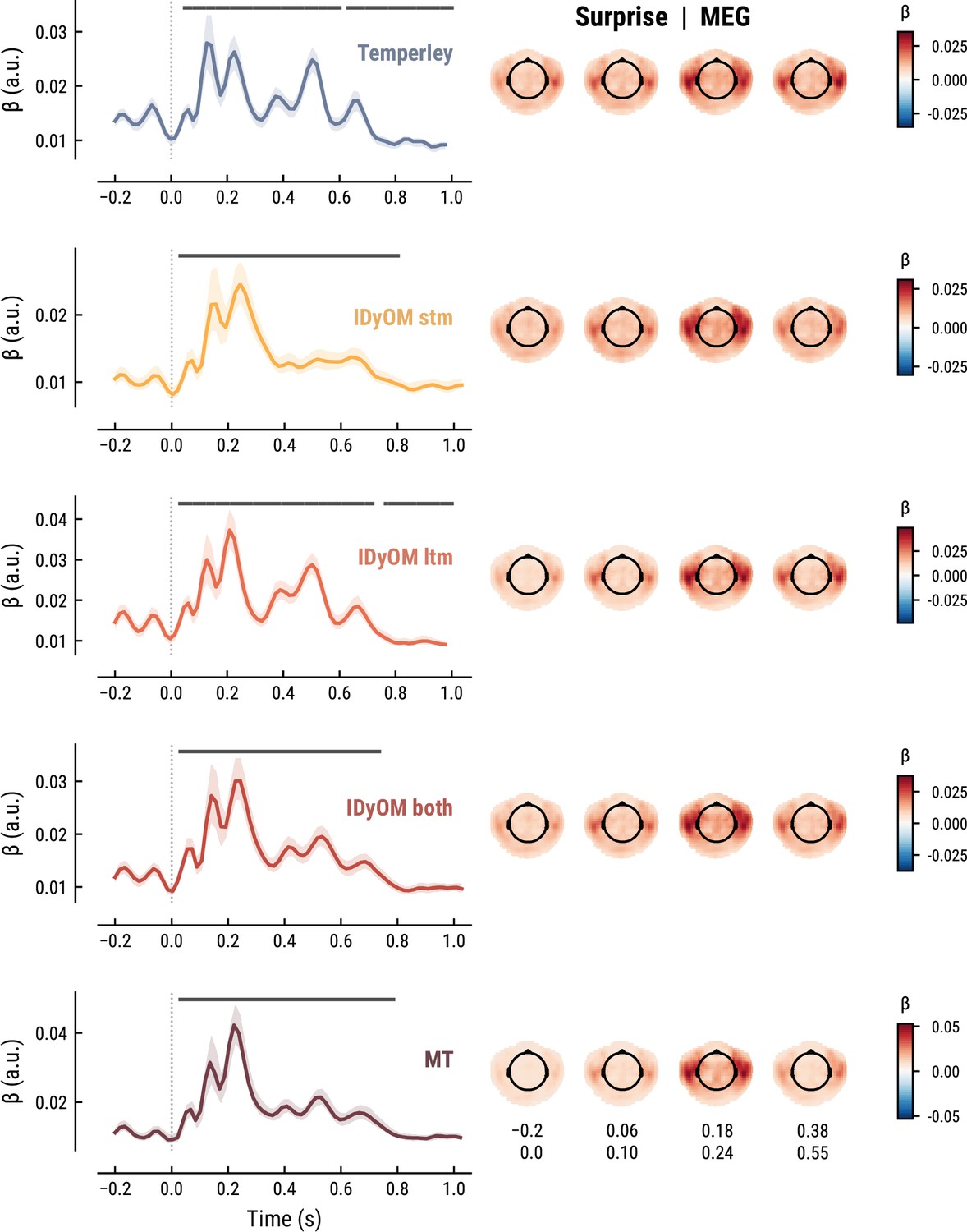
Comparison of the MEG TRFs and spatial topographies for the surprise estimates from the best models of each model class.
Appendix 1—figure 4
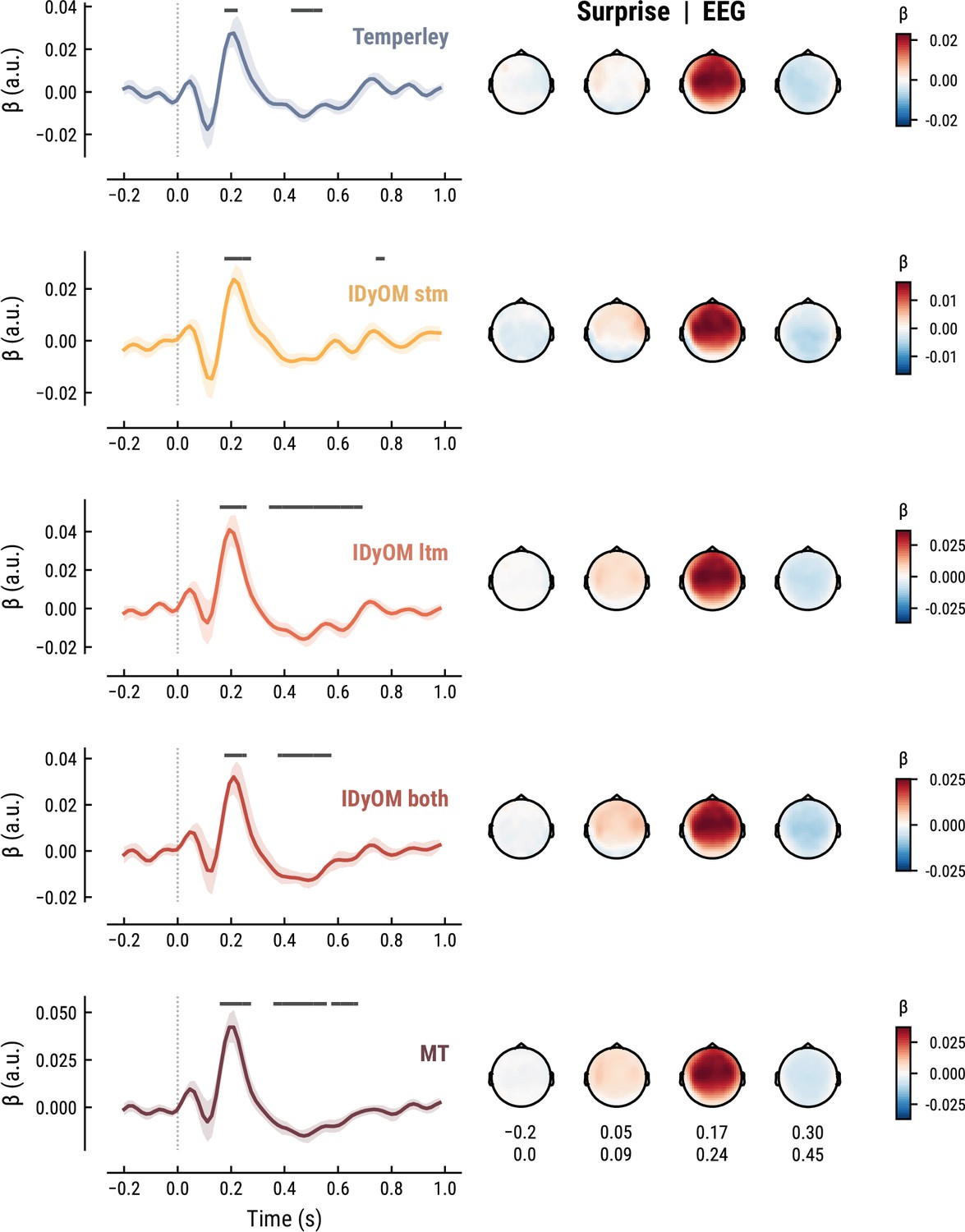
Comparison of the EEG TRFs and spatial topographies for the surprise estimates from the best models of each model class.
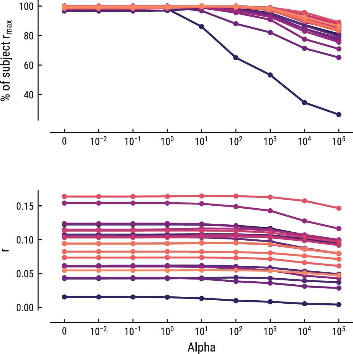
Appendix 1—figure 5
Comparison of the predictive performance on the MEG data using ridge-regularized regression, with the optimal cost hyperparameter alpha estimated using nested cross-validation.
Results are shown for the best-performing model (MT, context length of 8 notes). Each line represents one participant. Lower panel: raw predictive performance (r). Upper panel: predictive performance expressed as percentage of a participant’s maximum.
Appendix 1—figure 6
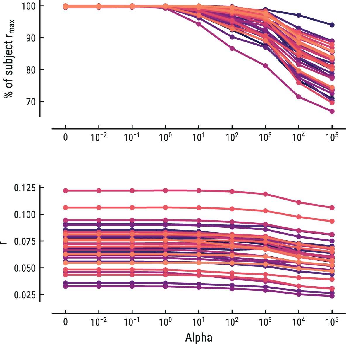
Comparison of the predictive performance on the EEG data using ridge-regularized regression, with the optimal cost hyperparameter alpha estimated using nested cross-validation.
Results are shown for the best-performing model (MT, context length of 7 notes). Each line represents one participant. Lower panel: raw predictive performance (r). Upper panel: predictive performance expressed as percentage of a participant’s maximum.
Author response image 1
Author response image 2
Tables
Appendix 1—table 1
Overview of the musical stimuli presented in the MEG (top) and EEG study (bottom).
| MusicMEG | ||||||||
|---|---|---|---|---|---|---|---|---|
| Composer | Composition | Year | Key | Time signature | Tempo (bpm) | Duration (sec) | Notes | Sound |
| Benjamin Britten | Metamorphoses Op. 49, II. Phaeton | 1951 | C maj | 4/4 | 110 | 95 | 384 | Oboe |
| Benjamin Britten | Metamorphoses Op. 49, III. Niobe | 1951 | Db maj | 4/4 | 60 | 101 | 171 | Oboe |
| Benjamin Britten | Metamorphoses Op. 49, IV. Bacchus | 1951 | F maj | 4/4 | 100 | 114 | 448 | Oboe |
| César Franck | Violin Sonata IV. Allegretto poco mosso | 1886 | A maj | 4/4 | 150 | 175 | 458 | Flute |
| Carl Philipp Emanuel Bach | Sonata for Solo Flute, Wq.132/H.564 III. | 1763 | A min | 3/8 | 98 | 275 | 1358 | Flute |
| Ernesto Köhler | Flute Exercises Op. 33 a, V. Allegretto | 1880 | G maj | 4/4 | 124 | 140 | 443 | Flute |
| Ernesto Köhler | Flute Exercises Op. 33b, VI. Presto | 1880 | D min | 6/8 | 176 | 134 | 664 | Piano |
| Georg Friedrich Händel | Flute Sonata Op. 1 No. 5, HWV 363b, IV. Bourrée | 1711 | G maj | 4/4 | 132 | 84 | 244 | Oboe |
| Georg Friedrich Händel | Flute Sonata Op. 1 No. 3, HWV 379, IV. Allegro | 1711 | E min | 3/8 | 96 | 143 | 736 | Piano |
| Joseph Haydn | Little Serenade | 1785 | F maj | 3/4 | 92 | 81 | 160 | Oboe |
| Johann Sebastian Bach | Flute Partita BWV 1013, II. Courante | 1723 | A min | 3/4 | 64 | 176 | 669 | Flute |
| Johann Sebastian Bach | Flute Partita BWV 1013, IV. Bourrée angloise | 1723 | A min | 2/4 | 62 | 138 | 412 | Oboe |
| Johann Sebastian Bach | Violin Concerto BWV 1042, I. Allegro | 1718 | E maj | 2/2 | 100 | 122 | 698 | Piano |
| Johann Sebastian Bach | Violin Concerto BWV 1042, III. Allegro Assai | 1718 | E maj | 3/8 | 92 | 80 | 413 | Piano |
| Ludwig van Beethoven | Sonatina (Anh. 5 No. 1) | 1807 | G maj | 4/4 | 128 | 210 | 624 | Flute |
| Muzio Clementi | Sonatina Op. 36 No. 5, III. Rondo | 1797 | G maj | 2/4 | 112 | 187 | 915 | Piano |
| Modest Mussorgsky | Pictures at an Exhibition - Promenade | 1874 | Bb maj | 5/4 | 80 | 106 | 179 | Oboe |
| Pyotr Ilyich Tchaikovsky | The Nutcracker Suite - Russian Dance Trepak | 1892 | G maj | 2/4 | 120 | 78 | 396 | Piano |
| Wolfgang Amadeus Mozart | The Magic Flute K620, Papageno’s Aria | 1791 | F maj | 2/4 | 72 | 150 | 452 | Flute |
| 2589 | 9824 | |||||||
| MusicEEG | ||||||||
| Composer | Composition | Year | Key | Time signature | Tempo (bpm) | Duration (sec) | Notes | Sound |
| Johann Sebastian Bach | Flute Partita BWV 1013, I. Allemande | 1723 | A min | 4/4 | 100 | 158 | 1022 | Piano |
| Johann Sebastian Bach | Flute Partita BWV 1013, II. Corrente | 1723 | A min | 3/4 | 100 | 154 | 891 | Piano |
| Johann Sebastian Bach | Flute Partita BWV 1013, III. Sarabande | 1723 | A min | 3/4 | 70 | 120 | 301 | Piano |
| Johann Sebastian Bach | Flute Partita BWV 1013, IV. Bourree | 1723 | A min | 2/4 | 80 | 135 | 529 | Piano |
| Johann Sebastian Bach | Violin Partita BWV 1004, I. Allemande | 1723 | D min | 4/4 | 47 | 165 | 540 | Piano |
| Johann Sebastian Bach | Violin Sonata BWV 1001, IV. Presto | 1720 | G min | 3/8 | 125 | 199 | 1604 | Piano |
| Johann Sebastian Bach | Violin Partita BWV 1002, I. Allemande | 1720 | Bb min | 4/4 | 50 | 173 | 620 | Piano |
| Johann Sebastian Bach | Violin Partita BWV 1004, IV. Gigue | 1723 | D min | 12/8_ | 120 | 182 | 1352 | Piano |
| Johann Sebastian Bach | Violin Partita BWV 1006, II. Loure | 1720 | E maj | 6/4 | 80 | 134 | 338 | Piano |
| Johann Sebastian Bach | Violin Partita BWV 1006, III. Gavotte | 1720 | E maj | 4/4 | 140 | 178 | 642 | Piano |
| 1598 | 7839 | |||||||
Additional files
Download links
A two-part list of links to download the article, or parts of the article, in various formats.
Downloads (link to download the article as PDF)
Open citations (links to open the citations from this article in various online reference manager services)
Cite this article (links to download the citations from this article in formats compatible with various reference manager tools)
Cortical activity during naturalistic music listening reflects short-range predictions based on long-term experience
eLife 11:e80935.
https://doi.org/10.7554/eLife.80935


