Efficient value synthesis in the orbitofrontal cortex explains how loss aversion adapts to the ranges of gain and loss prospects
- Sorbonne Université, France
- Institut du Cerveau, France
- INSERM UMR S1127, France
Figures
Figure 1 with 4 supplements
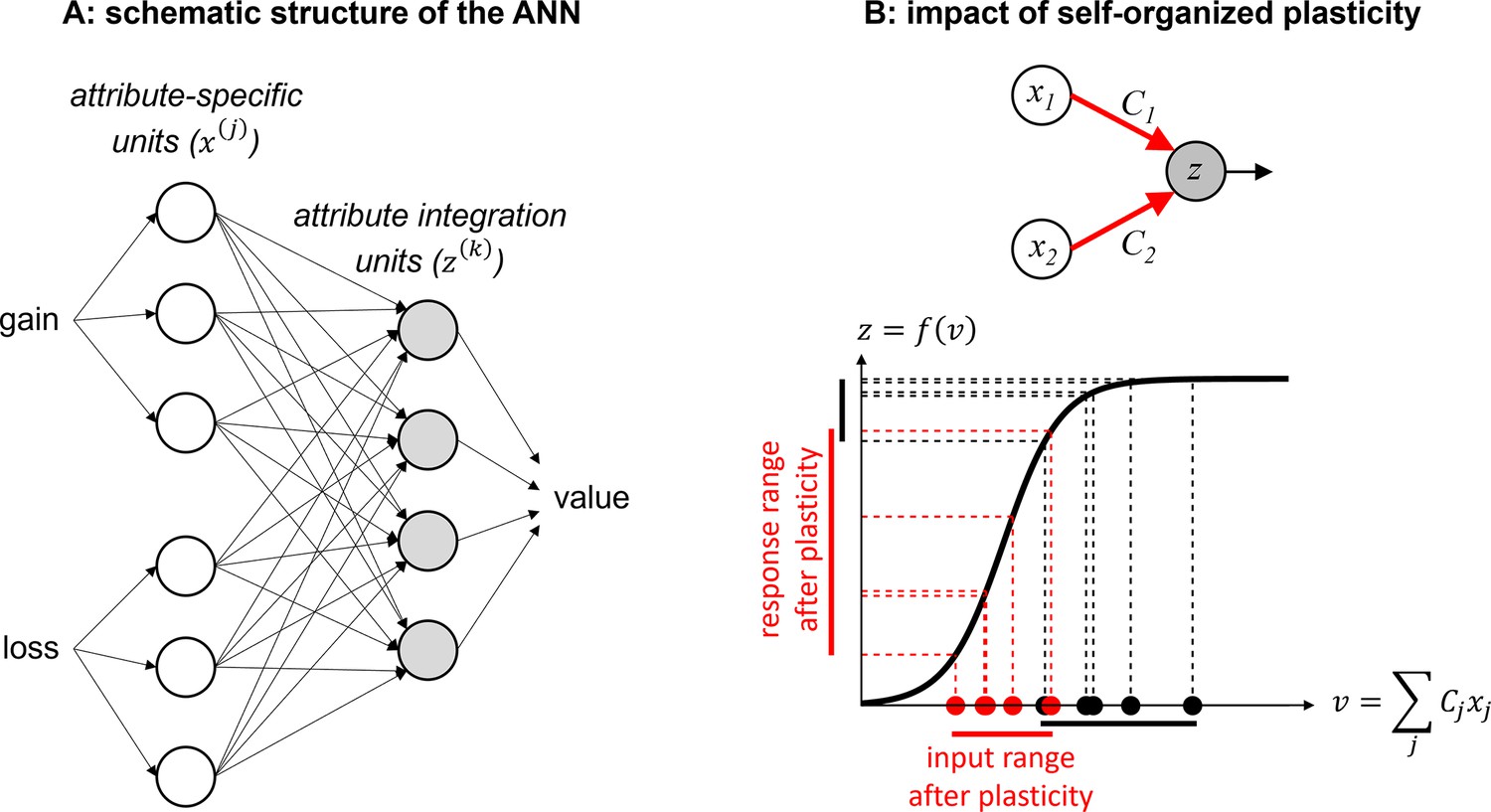
Efficient value synthesis.
(A) Schematic structure of the artificial neural network (ANN). Trial-by-trial prospective gains (G) and losses (L) first enter attribute-specific units (white circles), which then send their outputs to integration units (gray circles). The outputs of these units are then combined to yield trial-by-trial gamble values, using a linear population code. (B) The impact of self-organized plasticity on integration units’ response. Integration units receive a weighted mixture (v) of attribute units’ outputs (x), and their firing response is a sigmoidal mapping z=f(v) of their input. In principle, inputs to integration units (black dots) may sample the saturating range of their sigmoidal activation function (black vertical bar on the y-axis). However, self-organized plasticity modifies the connection strengths between attribute and integration units, such that the ensuing inputs to integration units (red dots) eventually fall within the responsive range of the activation function (red vertical bar on the y-axis).
Figure 1—figure supplement 1
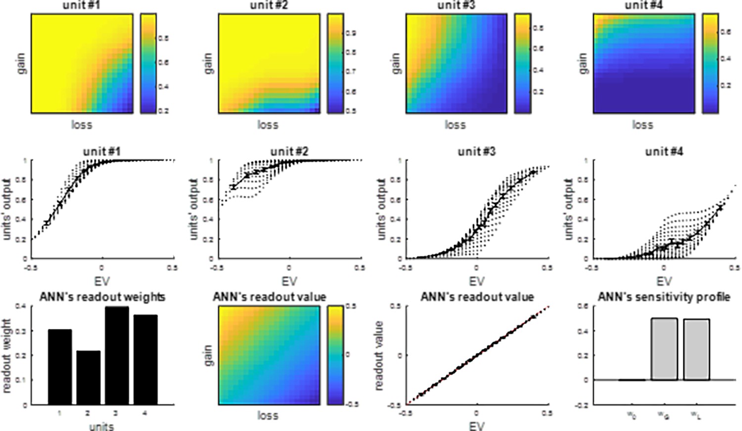
Summary of sigmoidal integration units’ response profiles.
Top row: the receptive field of each artificial neural network /(ANN) integration unit (color code: from blue -minimal output response- to yellow -maximal output response-) is displayed as a function of prospective losses (x-axis) and gains (y-axis). Middle row: the units’ output response (y-axis) is plotted against the gamble’s expected value (x-axis). Black dots show the possibly different response magnitudes of integration units for a given expected value (EV) (which may be obtained by different combinations of prospective gains and losses). Bottom row: ANN value readout weights (y-axis), ANN’s readout value profile (color code) displayed as a function of prospective losses (x-axis) and gains (y-axis), ANN’s readout value (y-axis) plotted as a function of EV (x-axis), and the ANN readout value’s sensitivity to prospective gains () and losses ().
Figure 1—figure supplement 2
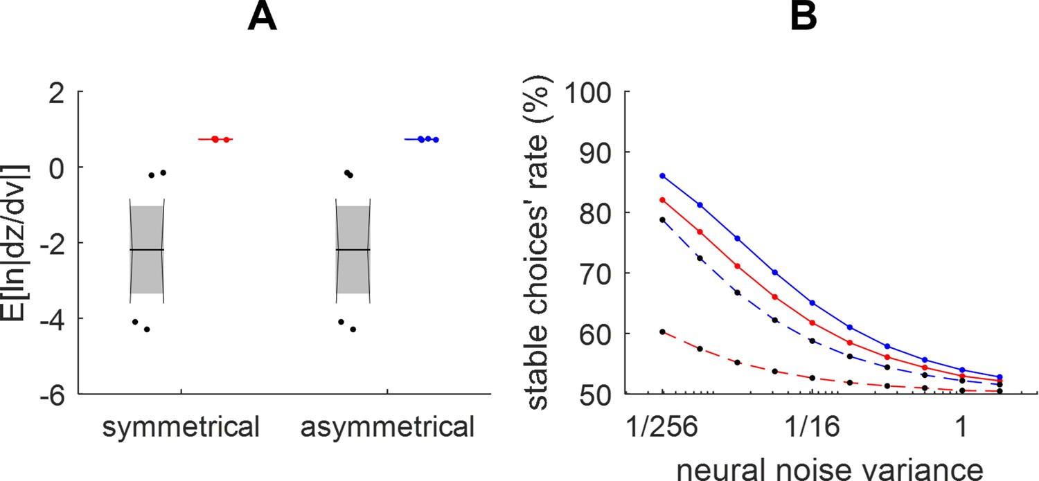
Efficiency of value synthesis.
(A) The expected log steepness of units’ activation functions (y-axis) is plotted before (black) and after self-organized plasticity for both the symmetrical (red) and asymmetrical (blue) gain/loss domains. (B) The stable choices’ rate (y-axis) is plotted as a function of neural noise variance, (x-axis) before (black dots and dotted lines) and after (plain lines) self-organized plasticity for both the symmetrical (red) and asymmetrical (blue) gain/loss domains.
Figure 1—figure supplement 3
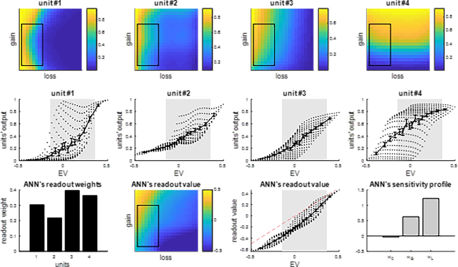
Summary of integration units’ response profiles after self-organized plasticity.
Same format as Figure 1. Top row: the black boxes depict the (‘wide’) domain of prospective gains and losses that are spanned during efficient integration. Middle row: the gray shaded areas depict the range of expected values (EVs) that corresponds to the spanned (‘wide’) domain of prospective gains and losses.
Figure 1—figure supplement 4
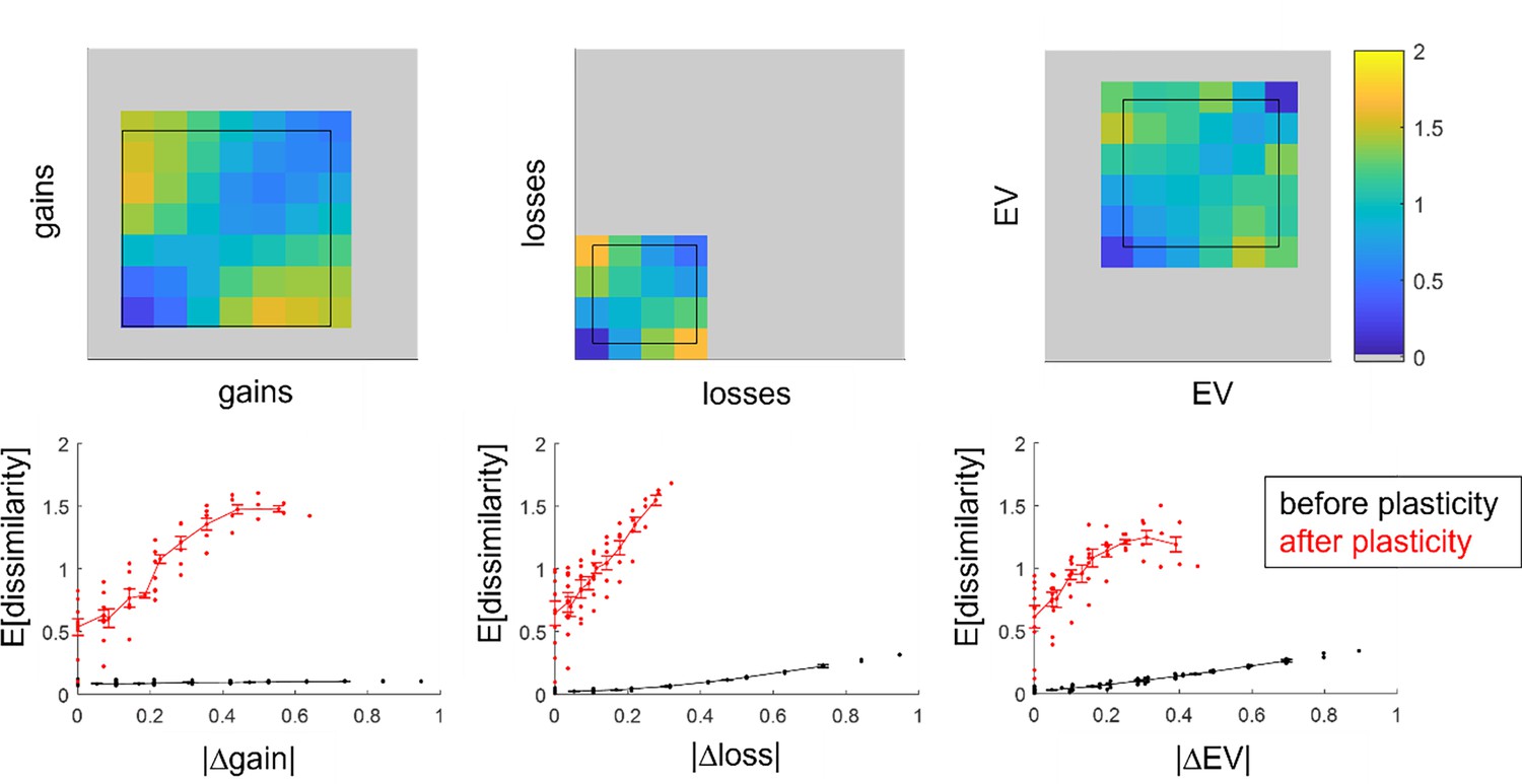
Analysis of the information content within the artificial neural networks (ANN’s) integration layer.
Upper panels: representational dissimilarity matrices after self-organized plasticity has modified the integration layer’s receptive fields (color code: from blue -minimal dissimilarity- to yellow -maximal dissimilarity-) are displayed as a function of either prospective gains, prospective losses, or expected value (EV) (from left to right, 10 bins, x-axis, and y-axis). The black boxes show the spanned range of either gains, losses or EV. Lower panels: average neural dissimilarity (y-axis) is plotted as a function of absolute difference in prospective gains, prospective losses, or EV (from left to right, x-axis), both before (black) and after (red) self-organized plasticity has modified the integration layer’s receptive fields.
Figure 2
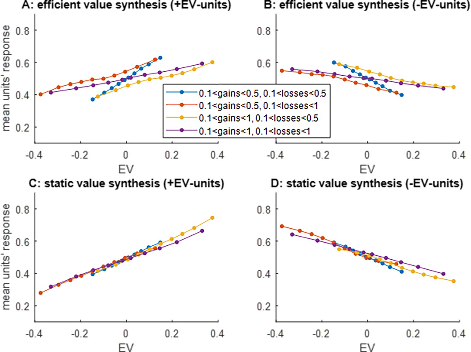
Apparent value range adaptation.
(A) The average units’ response (y-axis) to pairs of prospective gains and losses that fall within predefined expected value (EV) bins (x-axis) is shown, while artificial neural networks (ANNs) that operate efficient value synthesis are exposed to four different spanned gain/loss domains (blue: narrow ranges of gains and losses, violet: wide ranges of gains and losses, red: narrow gain range and wide loss range, yellow: wide gain range and narrow loss range, see main text). Only integration units that correlate positively with EV are shown. (B) integration units that correlate negatively with EV, same format as panel (A). C/D: same format as panels (A and B), for ANNs that operate static value synthesis.
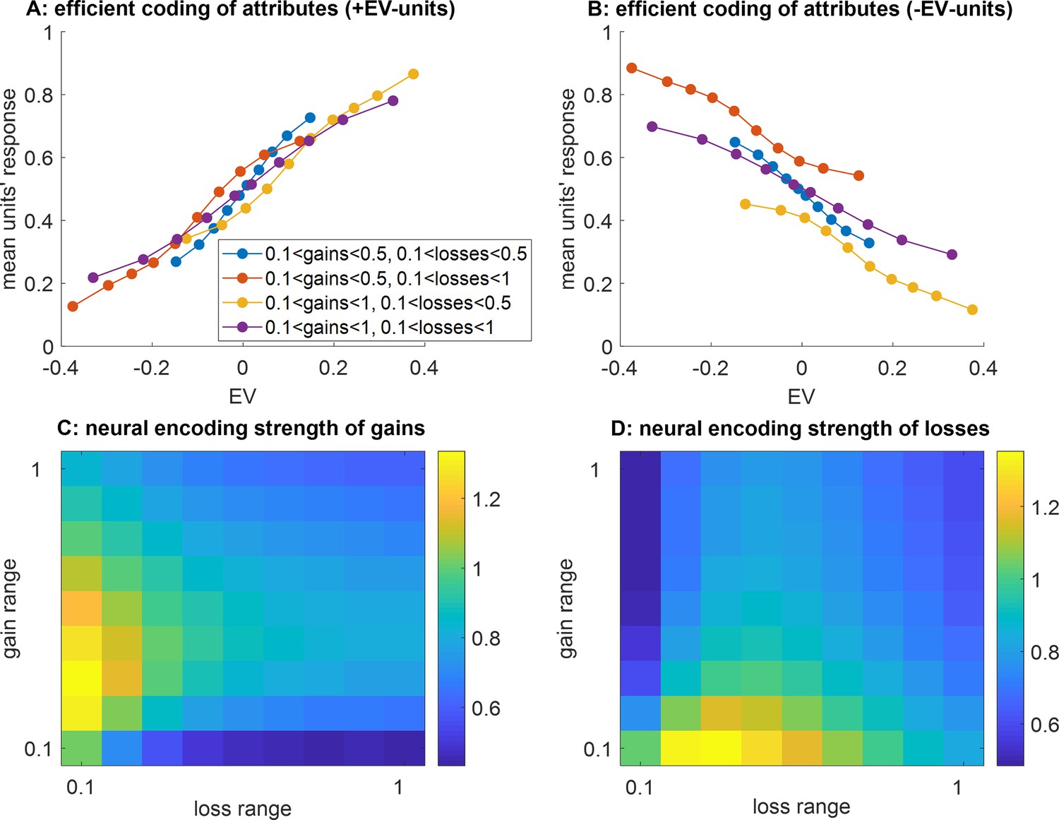
Figure 3
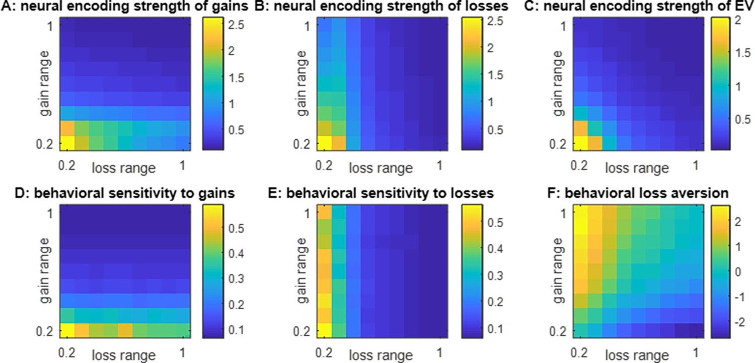
Impact of spanned ranges of gains and losses.
(A) The neural encoding strength of gains (color code: from blue -minimal encoding strength- to yellow -maximal encoding strength-) is shown as a function of the spanned range of losses (x-axis, range increases from left to right) and gains (y-axis, range increases from bottom to top). Note that the maximal range of prospective gains and losses is arbitrarily set to unity. (B) Neural encoding strength of losses, same format. (C) Neural encoding strength of EV, same format. (D) Behavioral sensitivity to gains, same format. (E) Behavioral sensitivity to losses, same format. (F) Behavioral loss aversion, same format.
Figure 4 with 1 supplement
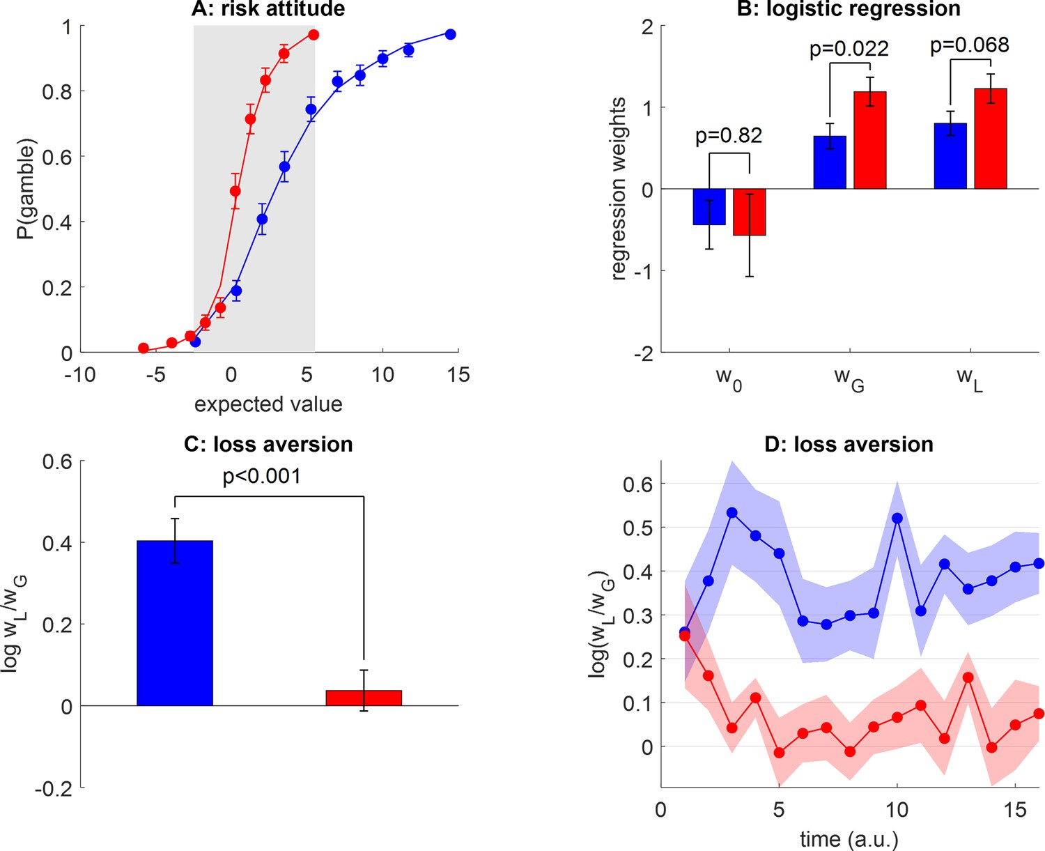
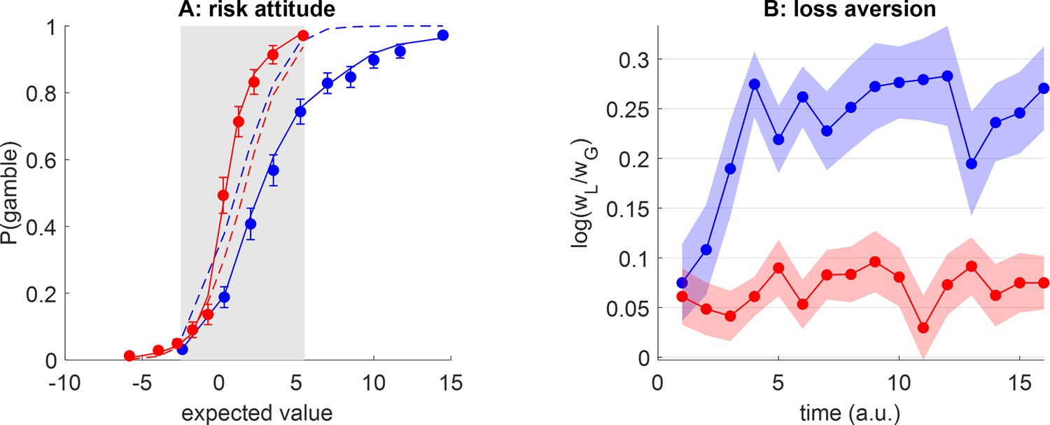
Do peoples’ loss aversion exhibit range adaptation?
(A) The group-average probability of gamble acceptance (y-axis) is plotted against deciles of gambles’ expected value (EV=(G–L)/2, x-axis), in both groups (red: narrow range, blue: wide range). Dots show raw data (error bars depict s.e.m.), and plain lines show predicted data under a logistic regression model (see main text). The gray-shaded area highlights the range of expected values that is common to both groups. (B) Estimates of gamble bias (w0) as well as sensitivity to gains (wG) and losses (wL) for both groups, under the logistic model (same color code as panel A, errorbars depict s.e.m.). (C) Average loss aversion (y-axis) is plotted for both groups (same color code, errorbars depict s.e.m.). (D) Temporal dynamics of group-average loss aversion (log wL/wG, y-axis, same color code) are plotted against time (a.u., x-axis). Shaded areas depict s.e.m.
Figure 4—figure supplement 1
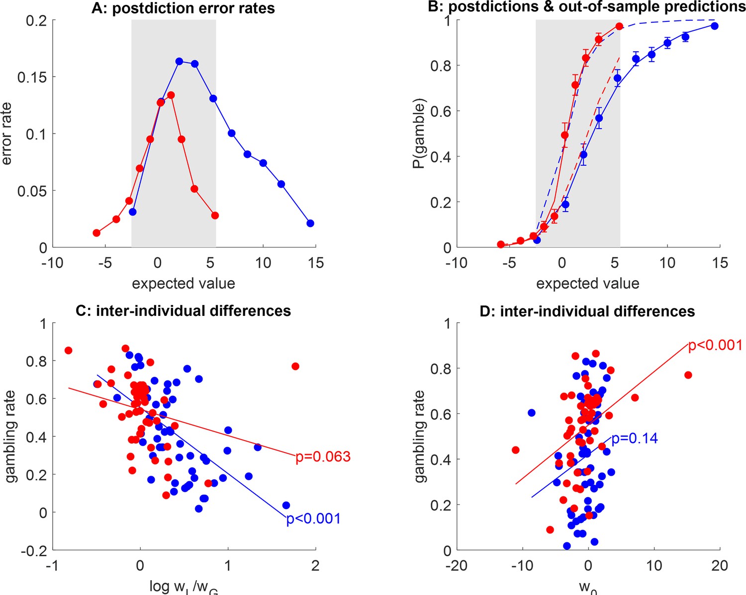
Postdiction error and out-of-sample predictions of the logistic model.
(A) ‘Postdiction’ error (y-axis) is plotted against deciles of gambles’ expected value (x-axis), in both groups (red: narrow range, blue: wide range). The gray-shaded area highlights the range of expected values that is common to both groups. (B) The probability of gamble acceptance (y-axis) is plotted against the gambles’ expected value (x-axis), in both groups (red: narrow range, blue: wide range). Dots show raw data (errorbars depict s.em.), and Plain and dashed lines show postdictions and out-of-sample predictions, respectively. (C) Peoples’ gambling rate within the common expected value (EV) range (y-axis) is plotted as a function of estimated loss aversion (x-axis), for each group of subjects. (D) People’s gambling rate within the common EV range (y-axis) is plotted as a function of estimated gambling bias (x-axis), same format.
Figure 5 with 1 supplement
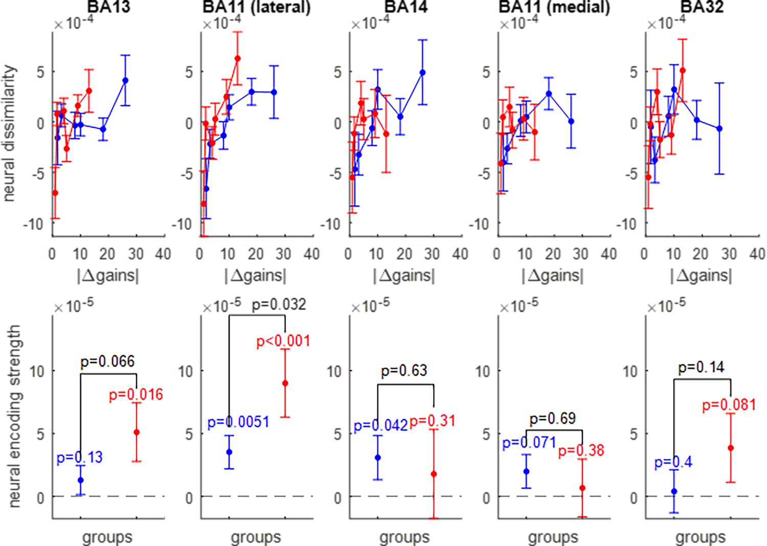
Neural encoding of prospective gains.
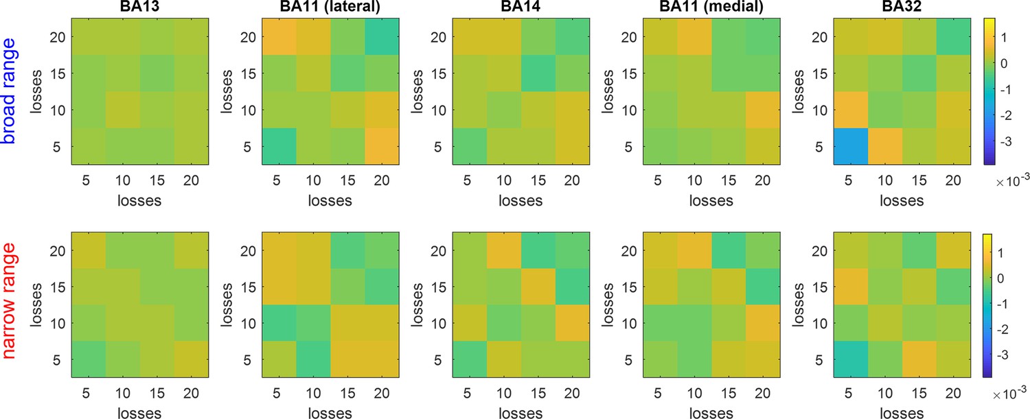
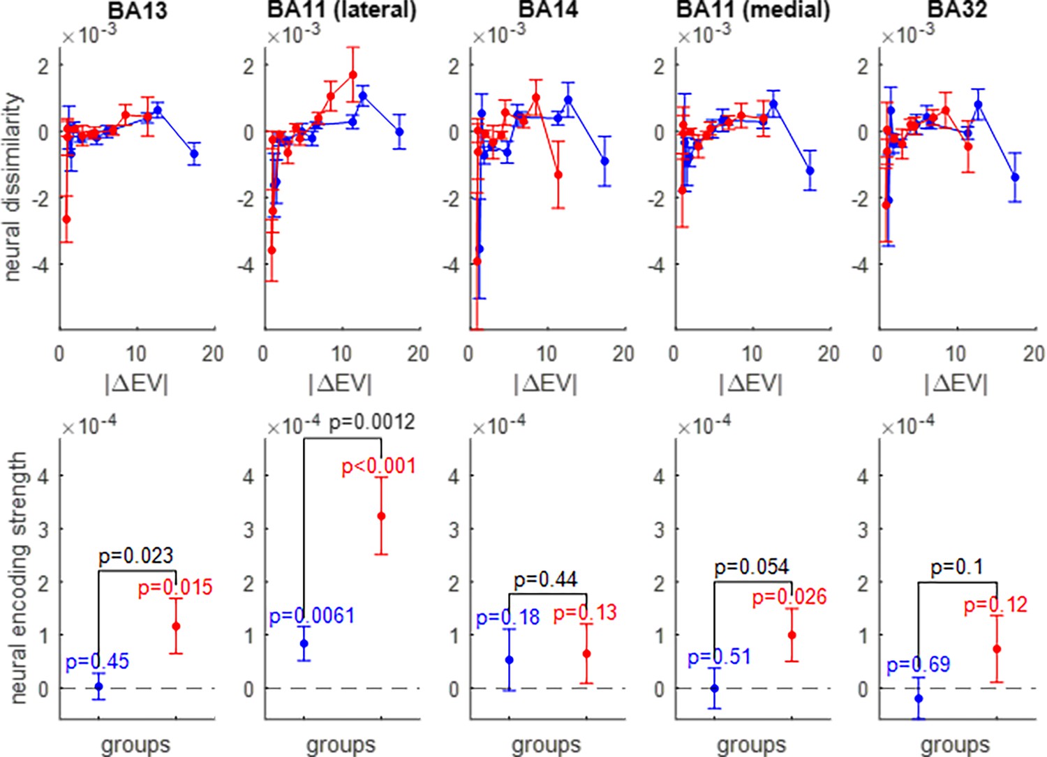
The upper panels show the trial-by-trial neural dissimilarity (y-axis) plotted as a function of trial-by-trial absolute difference in prospective gains (x-axis), for both groups of participants (red: narrow range, blue: wide range), and within each subregion of the OFC. The lower panels show the ensuing neural encoding strength of gains (y-axis), for both groups (same color code), and within each subregion of the OFC. The dotted line indicates the y-axis origin. Errorbars depict s.e.m., and p-values are uncorrected for multiple comparisons.
Figure 5—figure supplement 1
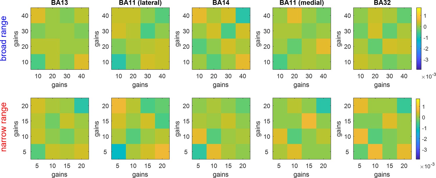
Gain-representational dissimilarity matrices (RDMs).
Average trial-by-trial neural dissimilarity is shown, having binned trials according to prospectives gains (average gains within bins increase from left to right and from bottom to top). Upper row: wide range group, lower row: narrow range group. Each column shows an OFC subregion (from left to right: medial part of BA13, lateral part of BA11, rostral part of BA14, medial part of BA11, rostral part of BA32). The color code is the same for all panels.
Figure 6 with 1 supplement
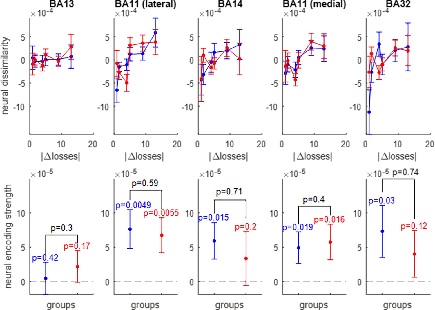
Neural encoding of prospective losses.
Same format as Figure 5.
Figure 6—figure supplement 1
Loss-representational dissimilarity matrices (RDMs).
Average trial-by-trial neural dissimilarity is plotted, having binned trials according to prospectives losses. Same format as Figure 9 (and the same color code).
Figure 7 with 2 supplements
Neural encoding of expected value (EV).
Same format as Figure 5.
Figure 7—figure supplement 1
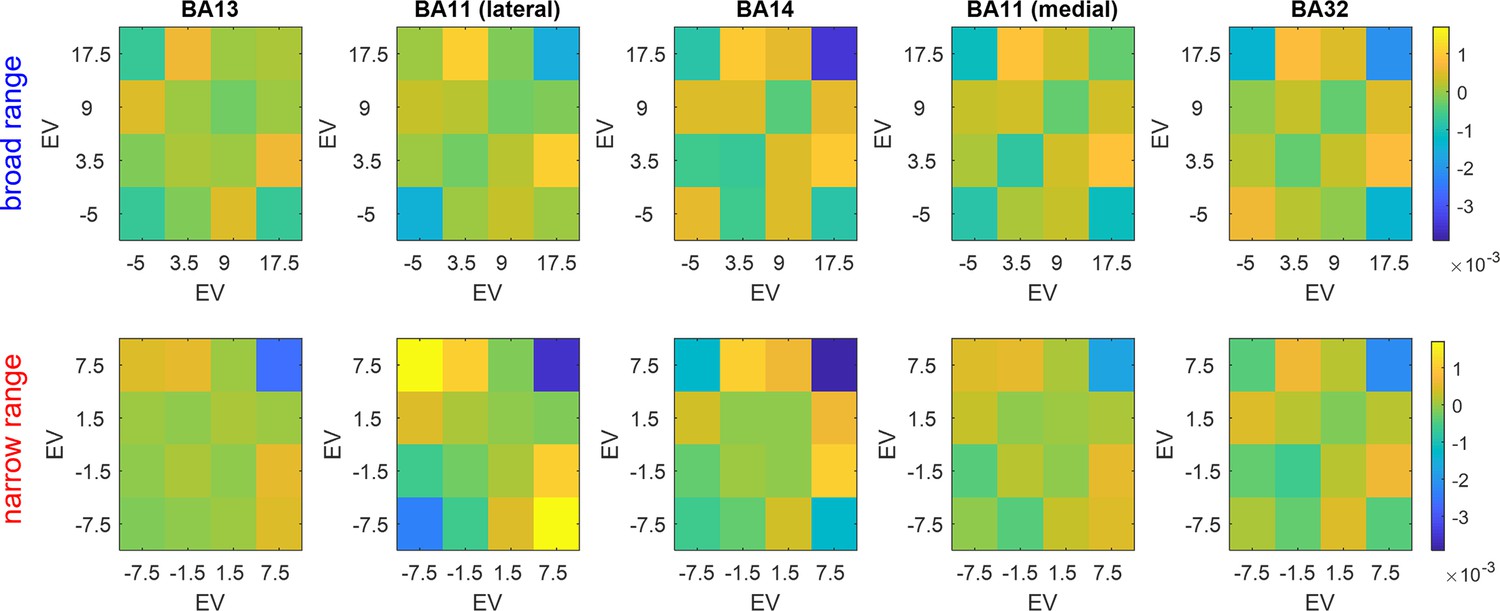
Expected value (EV)-representational dissimilarity matrices (RDMs).
Average trial-by-trial neural dissimilarity is plotted, having binned trials according to EVs. Same format as Figure 9 (and the same color code).
Figure 7—figure supplement 2
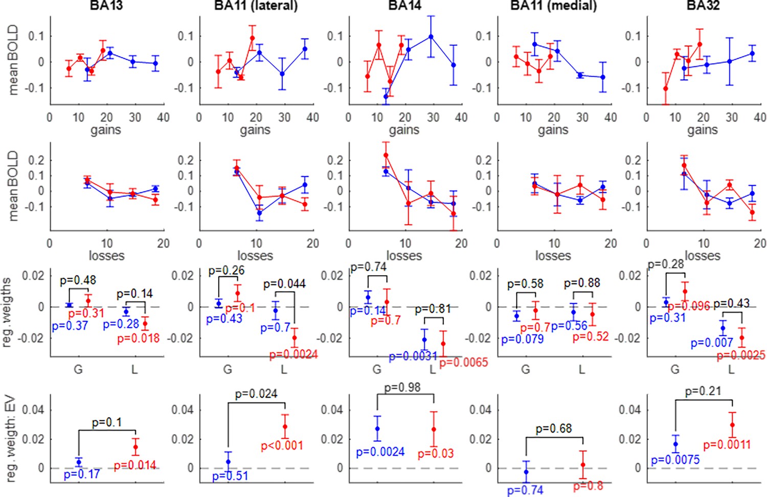
Univariate fMRI analyses.
First row: the average BOLD response (y-axis) is plotted as a function of prospective gains (x-axis), for both groups of participants (red: narrow group, blue: wide group). Second row: same as first row, for prospective losses. Third row: GLM parameter estimates (y-axis) for gains and losses. Fourth row: regression parameter estimates for expected value (EV). Each column shows an OFC subregion (from left to right: medial part of BA13, lateral part of BA11, rostral part of BA14, medial part of BA11, rostral part of BA32). The dashed black lines depict the y-axis origin.
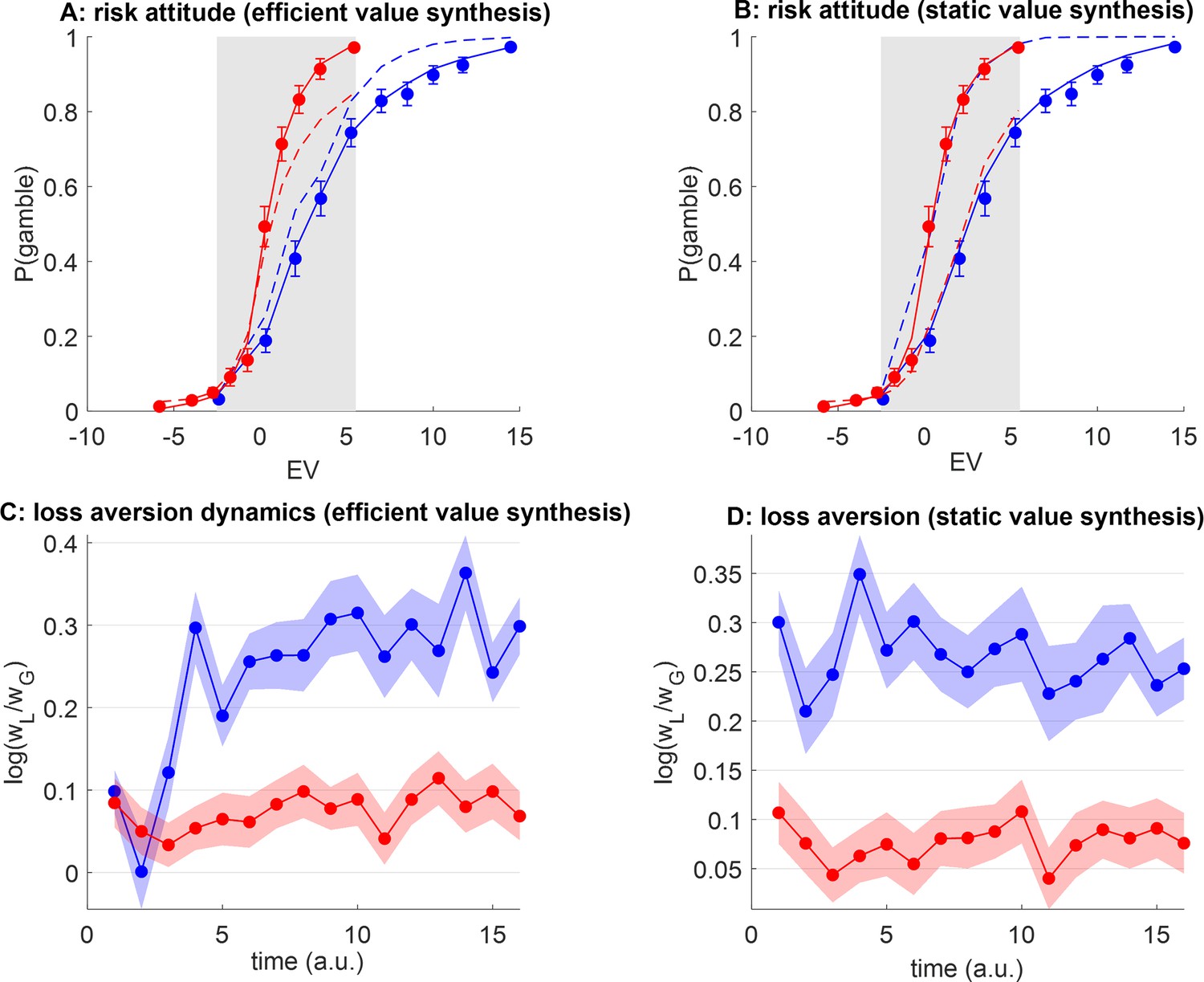
Figure 8 with 2 supplements
Efficient value synthesis: Artificial neural network (ANN) analysis of behavioral data.
(A) The probability of gamble acceptance under plastic ANNs (y-axis) is plotted against gambles’ expected value (EV) (x-axis), in both groups (red: narrow range, blue: wide range). Dots show raw data (error bars depict s.em.). Plain and dashed lines show postdiction and out-of-sample predictions (see main text), respectively. The gray-shaded area highlights the range of expected values that is common to both groups. (B) Same as panel A, for static ANN. (C) Postdicted loss aversion (y-axis) is plotted as a function of time (x-axis) for both groups (same color code), under the efficient value synthesis model. (D) Same as panel C, for static value synthesis.
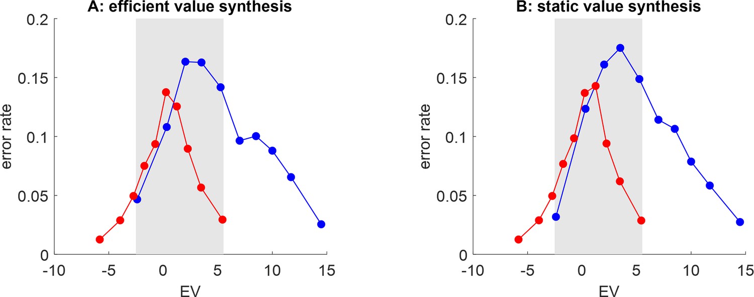
Figure 8—figure supplement 1
Artificial neural network (ANNs’) postdiction error rate.
(A) The rate of postdiction error (y-axis) under the efficient value synthesis scenario is plotted against gambles’ expected value (x-axis), for both groups (red: narrow range, blue: wide range). (B) Static value synthesis, same format.
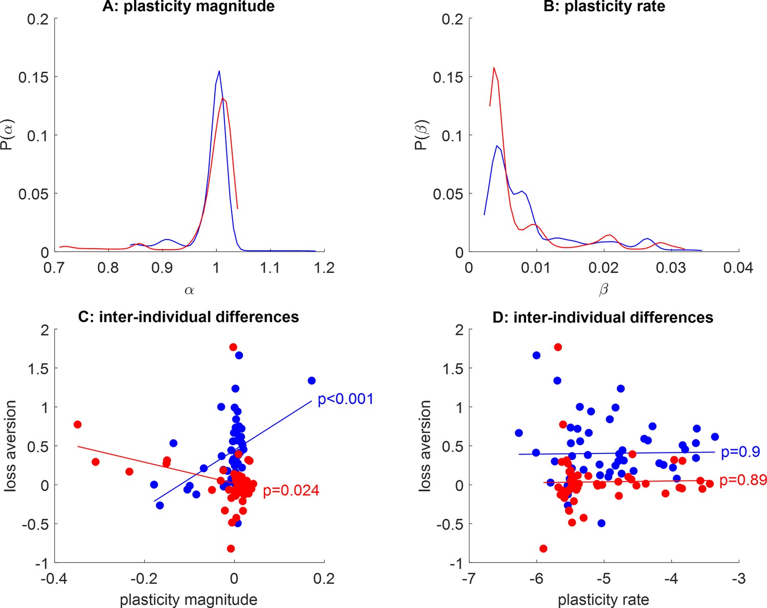
Figure 8—figure supplement 2
Self-organized plasticity parameter estimates.
(A) Empirical distribution of plasticity magnitude, for both groups (red: narrow range, blue: wide range). (B) Empirical distribution of plasticity rate. (C) Observed loss aversion (y-axis) is plotted as a function of plasticity magnitude (x-axis, log scale), for both groups. Each dot is a participant; plain lines depict the best-fitting linear trend. (D) Observed loss aversion as a function of plasticity rate (log scale).
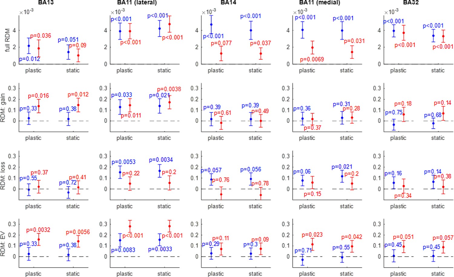
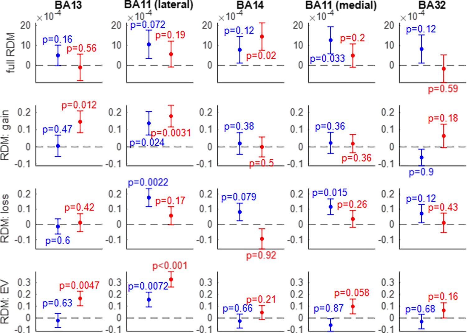
Figure 9 with 1 supplement
Efficient value synthesis: Representational similarity analysis (RSA) analysis results.
Within each panel, the correlation between artificial neural network (ANN)-based and fMRI-based representational dissimilarity matrices (RDMs) (y-axis) is shown for both groups of participants (red: narrow range group, blue: wide range group), and both ANN variants (left: plastic ANN, right: static ANN). Errorbars depict within-group s.e.m., and p-values are uncorrected for multiple comparisons. Each column shows the representational similarity analysis (RSA) results of a given OFC subregion from left to right: BA13 (medial), BA11 (lateral), BA14 (rostral), BA11 (medial), and BA32 (rostral). Each row shows one type of RDM (from top to bottom: trial-by-trial RDMs, gain-RDMs, loss-RDMs, and expected value (EV)-RDMs).
Figure 9—figure supplement 1
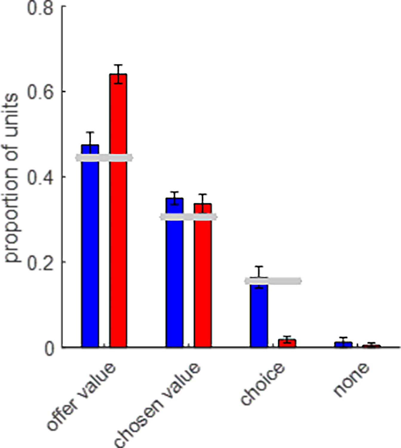
Response profile diversity in HP-artificial neural networks (ANNs’) integration units.
The average proportion of HP-ANNs integration units (y-data) that shows a significant correlation with choice, chosen value, and offer value (or none of these) is plotted for both groups (blue: wide range, red: narrow range). Error bars depict s.e.m. (across participants). Horizontal gray bars show the normalized frequency of ‘offer value,’ ‘chosen value,’ and ‘choice’ cells detected at OFC neurons’ response peak (see Figure 4 in Padoa-Schioppa and Assad, 2006).
Figure 10 with 3 supplements
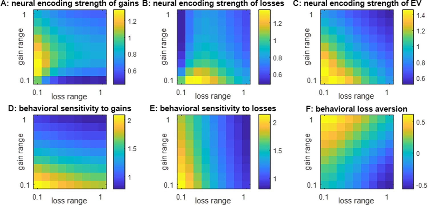
Main divergent predictions of the efficient coding of attributes scenario.
(A) The average units’ response (y-axis) to pairs of prospective gains and losses that fall within predefined expected value (EV) bins (x-axis) is shown, while ANNs that operate efficient value synthesis are exposed to four different spanned gain/loss domains (blue: narrow ranges of gains and losses, violet: wide ranges of gains and losses, red: narrow gain range and wide loss range, yellow: wide gain range and narrow loss range, see main text). Only integration units that correlate positively with EV are shown. (B) Integration units that correlate negatively with EV, same format as panel (A). (C) The neural encoding strength of gains (color code: from blue -low encoding strength- to yellow -high encoding strength-) is shown as a function of the spanned range of losses (x-axis, range increases from left to right) and gains (y-axis, range increases from bottom to top). (D) Neural encoding strength of losses, same format.
Figure 10—figure supplement 1
Efficient coding of attributes: impact of spanned ranges of gains and losses.
(A) The neural encoding strength of gains (color code: from blue -minimal encoding strength- to yellow -maximal encoding strength-) is shown as a function of the spanned range of losses (x-axis, range increases from left to right) and gains (y-axis, range increases from bottom to top). (B) Neural encoding strength of losses, same format. (C) Neural encoding strength of expected value (EV), same format. (D) Behavioral sensitivity to gains, same format. (E) Behavioral sensitivity to losses, same format. (F) Behavioral loss aversion, same format.
Figure 10—figure supplement 2
Efficient coding of attributes: Artificial neural network (ANN) analysis of behavioral data.
(A) The probability of gamble acceptance (y-axis) is plotted against the gambles’ expected value (EV) (x-axis), in both groups (red: narrow range, blue: wide range). Dots show raw data (error bars depict s.em.). Plain and dashed lines show postdictions and out-of-sample predictions (see main text), respectively. The gray-shaded area highlights the range of expected values that is common to both groups. (B) Postdicted loss aversion (y-axis) is plotted as a function of time (x-axis) for both groups (color code).
Figure 10—figure supplement 3
Efficient coding of attributes: Representational similarity analysis (RSA) analysis results.
Within each panel, the correlation between artificial neural network (ANN)-based and fMRI-based representational dissimilarity matrices (RDMs) (y-axis) is shown for both groups of participants (red: narrow range, blue: wide range). Error bars depict within-group s.e.m. Each column shows the representational similarity analysis (RSA) results of a given OFC subregion from left to right: BA13 (medial), BA11 (lateral), BA14 (rostral), BA11 (medial), and BA32 (rostral). Each row shows one type of RDM (from top to bottom: full-RDMs, gain-RDMs, loss-RDMs, and expected value (EV)-RDMs).
Figure 11
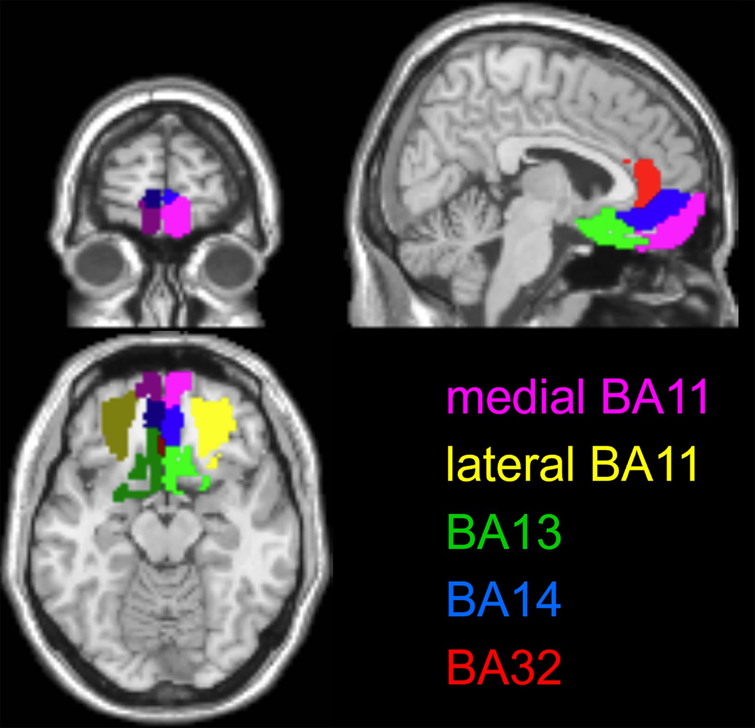
Anatomical masks of OFC subregions.
Pink: medial part of BA11, yellow: lateral part of BA11, green: A13, blue: BA14, red: BA32. Dark and light colors correspond to left and right hemispheric analogous regions, respectively.
Tables
Table 1
Anatomical coordinates of OFC subregions’ barycenter.
| Anatomical region | Barycenter coordinates (left) | Barycenter coordinates (right) |
|---|---|---|
| Medial part of BA11 | 68,166,125 | 114,164,126 |
| Lateral part of BA11 | 81,146,127 | 100,149,127 |
| BA13 | 81,146,127 | 100,149,127 |
| BA14 | 84,182,114 | 97,176,114 |
| Subgenual part of BA32 | 87,167,110 | 96,169,101 |
Appendix 1—table 1
Parameters' priors for biologically constrained artificial neural networks (ANNs).
| Parameter | Distributions | Rational |
|---|---|---|
| Firing rate threshold | Regular tiling of inputs | |
| Activation function slope | Partially overlapping tiling of inputs | |
| Initial connectivity | EV population code | |
| Value readout weights | EV population code | |
| Plasticity magnitude | Non informative prior | |
| Plasticity rate | Non informative prior |
Appendix 1—table 2
Mean R2 and its standard deviation for each model, for both groups.
| Narrow range group | Wide range group | |||
|---|---|---|---|---|
| Mean | Std | Mean | Std | |
| Logistic | 0.74 | 0.02 | 0.66 | 0.02 |
| Static ANN | 0.73 | 0.02 | 0.62 | 0.03 |
| Plastic ANN | 0.75 | 0.02 | 0.66 | 0.02 |
Additional files
Download links
A two-part list of links to download the article, or parts of the article, in various formats.
Downloads (link to download the article as PDF)
Open citations (links to open the citations from this article in various online reference manager services)
Cite this article (links to download the citations from this article in formats compatible with various reference manager tools)
Efficient value synthesis in the orbitofrontal cortex explains how loss aversion adapts to the ranges of gain and loss prospects
eLife 13:e80979.
https://doi.org/10.7554/eLife.80979


