A visual sense of number emerges from divisive normalization in a simple center-surround convolutional network
- Department of Psychological and Brain Sciences, University of Massachusetts Amherst, United States
- Commonwealth Honors College, University of Massachusetts Amherst, United States
Figures
Figure 1
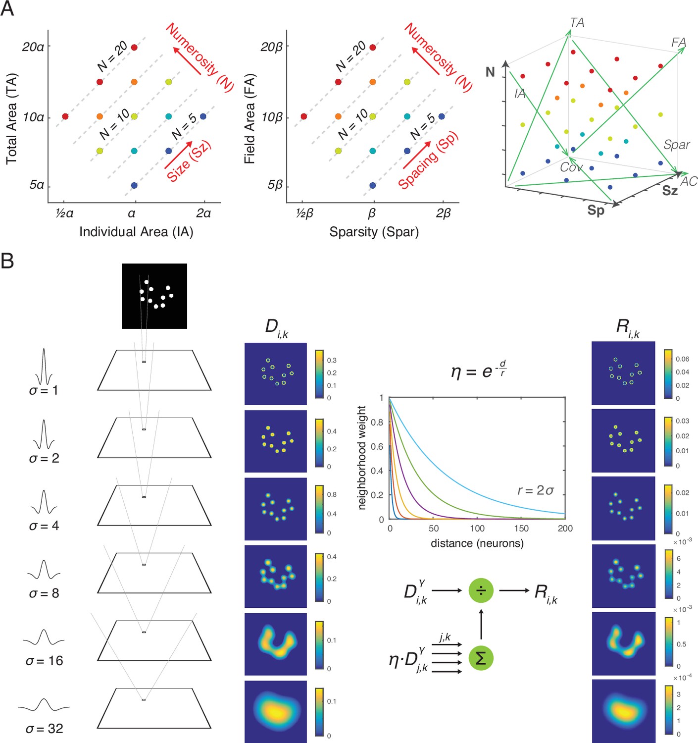
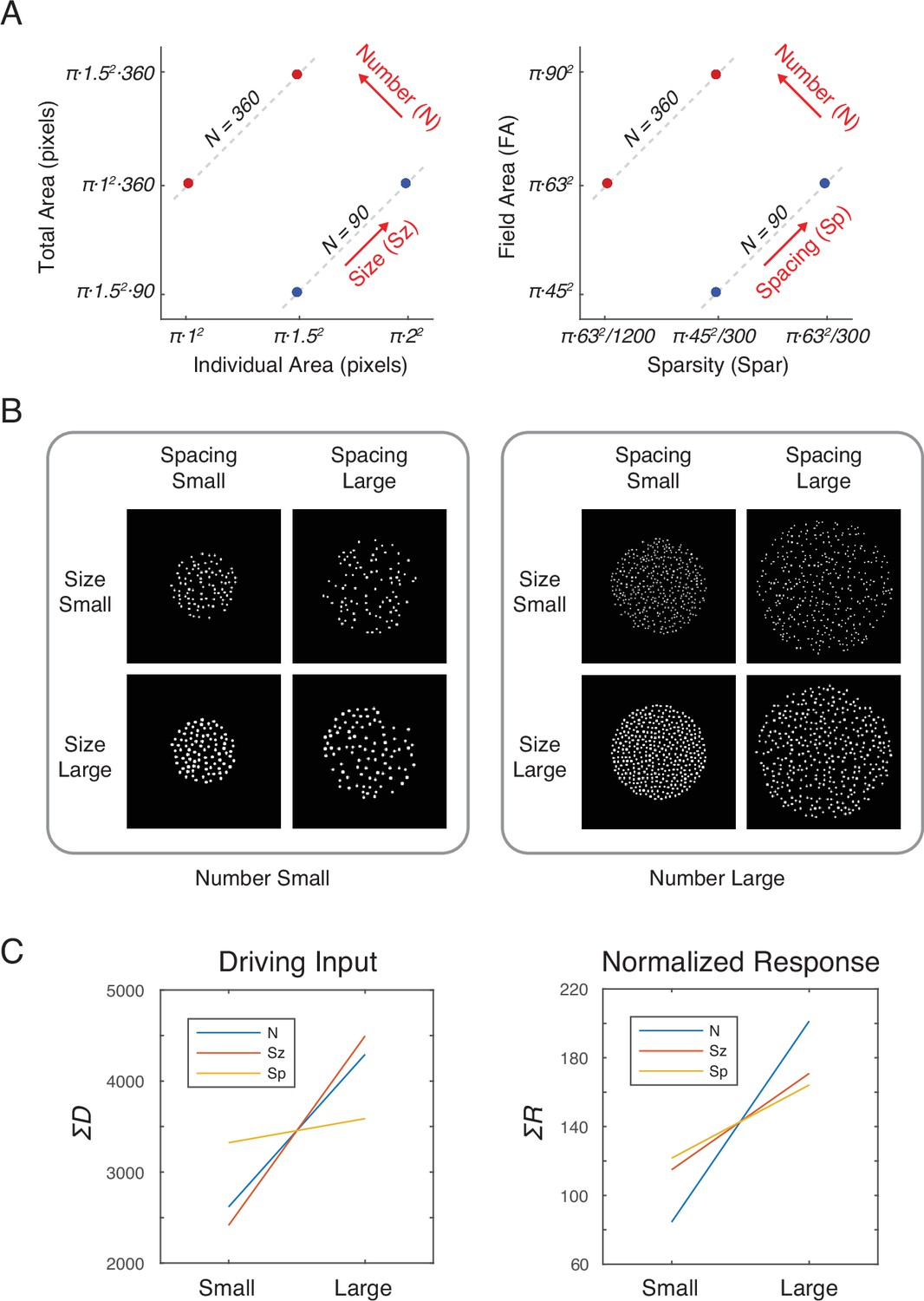
Stimulus design and computational methods.
(A) Properties of magnitude dimensions represented in three orthogonal axes defined by log-scaled number (N), size (Sz), and spacing (Sp) (Table 1). (B) Schematic illustration of the computational process from a dot-array image to the driving input (i.e., the model without divisive normalization), D, of the simulated neurons, versus the normalized response (i.e., the model with divisive normalization), R. A bitmap image of a dot array was fed into a convolutional layer with DoG filters in six different sizes (Equation 1). The resulting values, after half wave rectification, represented the driving input. Neighborhood weight, defined by η, was multiplied by the driving input across all the neurons across all the filter sizes, the summation of which served as the normalization factor (see Equations 2 and 3). This illustration of η is showing the case where r is defined by twice the size of the sigma for the DoG kernel. DOG, difference-of-Gaussians.
Figure 2 with 3 supplements
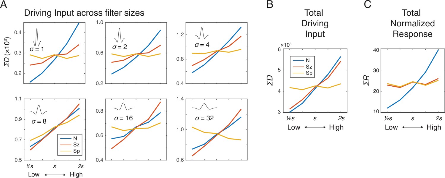
Simulation results showing the effects of number (N), size (Sz), and spacing (Sp) on the driving input and normalized response of the network units.
(A) Summed driving input (ΣD) separately for each of the six filter sizes as a function of N, Sz, and Sp (see Materials and methods for the specific values of s). (B) ΣD across all filters is modulated by both number and size but not by spacing. (C) Summed normalized response (ΣR) showed a near elimination of the Sz effect leaving only the effect of N. The results were simulated using r=2σ and γ=2, but effects of Sz and Sp were negligible across all the tested model parameters (Figure 2—figure supplement 2). The value s on the horizontal axis indicates a median value for each dimension (see Materials and methods).
Figure 2—figure supplement 1
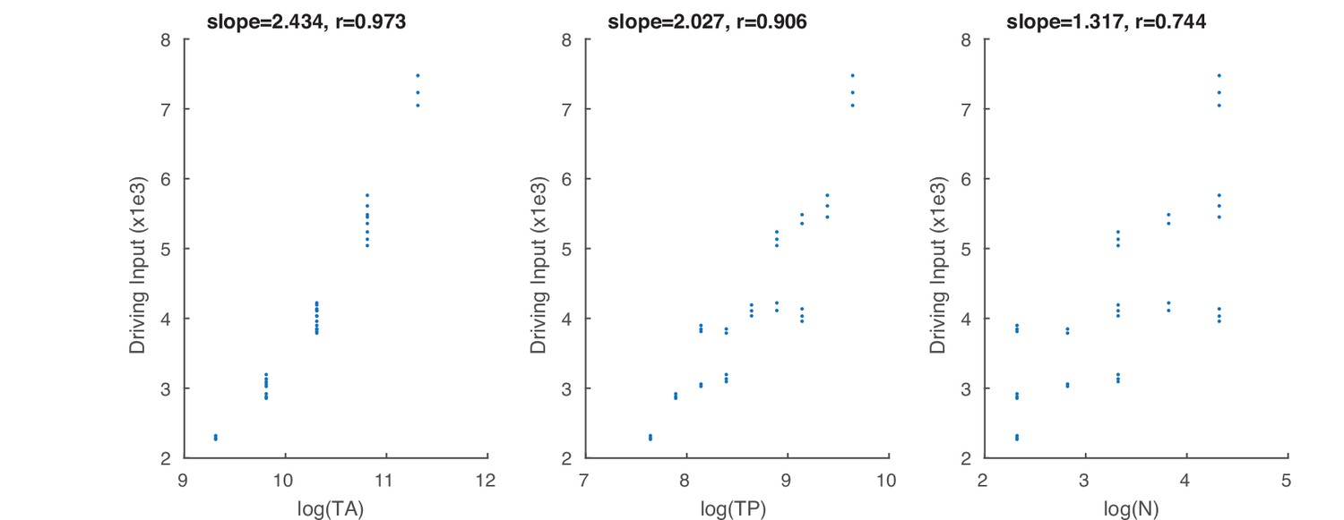
Additional illustration concerning the driving input.
Correlation between summed driving input, ΣD, and log-scaled total area (TA), total perimeter (TP), and number (N).
Figure 2—figure supplement 2
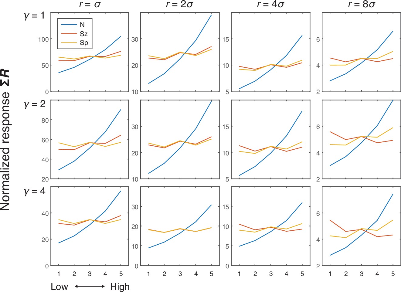
Simulation results showing the effects of number (N), size (Sz), and spacing (Sp) on the normalized response (i.e., the model with divisive normalization) of the network units as a function of neighborhood size (r) and amplification factor (γ).
Greater r resulted in a flatter curve for the size effect, and this flattening became more pronounced as γ increased, with the combination of high values for both parameters producing a modest negative effect of size as well as a modest positive effect of spacing. More specifically, the combination of high r and γ values produces a winner-take-all process across large regions of the display. Greater size, in these cases, thus leads to greater normalization factor (denominator) which results in reduced normalization activity, although the extent of this normalization depends on how far away the other dots are located (e.g., less normalization with spacing). Although this is an interesting phenomenon, empirical neural and behavioral studies show a positive effect of size, if any. Hence, larger values of r and γ in this model do not seem to be plausible in the case of numerosity perception. Therefore, we chose moderate values of r (=2) and γ (=2) for subsequent simulations.
Figure 2—figure supplement 3
Simulation results from images of densely packed dot arrays with extremely high numerosity.
(A) The dots arrays were systematically constructed ranging equally across the dimensions of N, Sz, and Sp, which was achieved by using the following parameters: number (n)=from 90 to 360, dot radius (rd)=from 1 to 2 pixels, field radius (rf)=from 45 to 90 pixels. For each point in the 2×2×2 parameters space, 16 unique arrays were created. (B) Examples of dot array images are shown. These images were submitted to the current computational model with the same parameters used in our original analysis (r=2σ and γ=2). (C) Summed driving input (ΣD) was modulated primarily by N and Sz. Summed normalized response (ΣR) was most modulated by N but also by Sz and Sp to some degree. The slope of the linear fit to N, Sz, and Sp adjusted by the baseline (the slope estimate divided by the intercept estimate in the simple regression) was 0.4086, 0.1958, and 0.1488, respectively. Note that this baseline-adjusted slope allows comparison of relative change in the response driven by N, Sz, and Sp, despite differences in the baseline activity across different sets of images. In our original simulation, the baseline-adjusted slopes for N, Sz, and Sp were 0.5771, 0.0646, and 0.0321, respectively. Thus, the same computational network when representing much more densely packed dot arrays seems to show relatively decreased sensitivity to numerosity. These results indicate that neural sensitivity to various magnitude dimensions and the degree of that sensitivity differ based on the assumptions about the distribution of filters and filter sizes.
Figure 3 with 7 supplements

Simulation of numerosity illusions.
Normalized response of the network units influenced by the (A) regularity, (B) grouping, and (C) heterogeneity of dot arrays, as well as by (D) adaptation and (E) context. Error bars represent one standard deviation of the normalized response across simulations; however, the error bars in most cases were too small to be visualized. Spatial normalization effects (A, B, and C) were simulated with r=2 and γ=2. Temporal normalization effects (D, E) used these same parameters values in combination with ω=8 and δ=1.
Figure 3—figure supplement 1
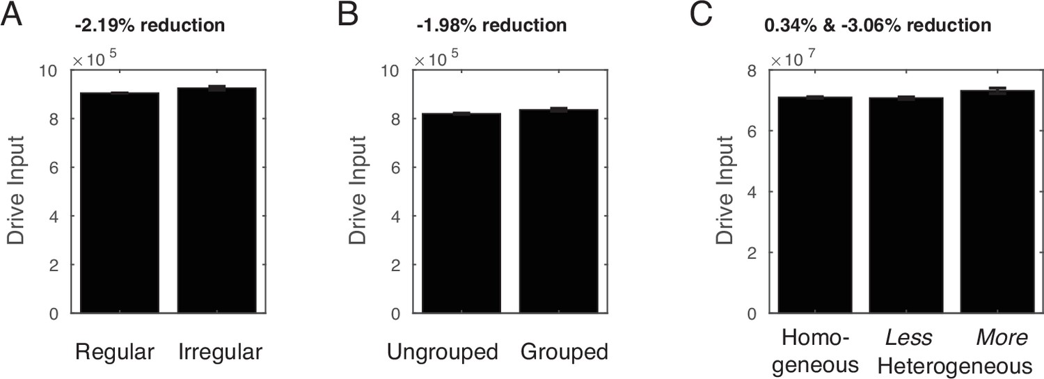
Simulation of visual illusions considering the driving input (i.e., the model without divisive normalization).
No underestimation was observed in any of these cases. If any, irregularly spaced arrays (by 2.19%), grouped arrays (by 1.98%), and more heterogeneous arrays (by 3.06%) were overestimated based on their driving input. In sum, without divisive normalization, the model failed to explain the typically observed visual illusions. Error bars indicate one standard deviation of the normalized response across 16 simulations.
Figure 3—figure supplement 2
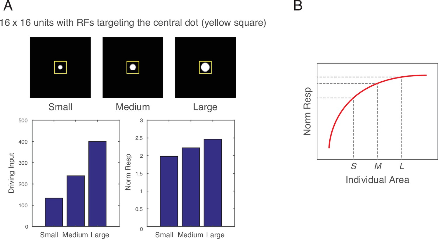
Effects of single dots.
(A) Images of small (radius=3.5), medium (radius=5), and large (radius=7) singly presented dots were fed into the computational model, and the driving input and the normalized response of the units with the receptive fields (RFs) targeting the dots were computed. As expected, driving input was nearly perfectly correlated with area of the dots (r=0.9983). In contrast, normalized response showed a linear relationship with the radius, which meant a logarithmic relationship with area. This occurs because a larger dot involves a greater number of filters overlapping with the dot (i.e., greater driving input), but this greater number of filters leads to a greater normalization factor (increase in the denominator of divisive normalization). In other words, the normalized response becomes tempered in a non-linear way, producing a saturating normalized response as a function of increasing dot area. (B) Schematic illustration of the saturating effect of normalized response for a single dot (within a hypothetical dot array) as a function of the area of the dot. Heterogeneous arrays are created by holding the total area and numerosity constant while changing individual dot size. Therefore, when medium-sized dots (M) are replaced with large dots (L), the same number of replacements must be done to go from medium-size dots (M) to small dots (S). However, because of the saturating effect, there is a greater decrease in normalized response than an increase in normalized response. Thus, the overall normalized response becomes necessarily smaller in a heterogeneous array compared to a homogeneous array.
Figure 3—figure supplement 3
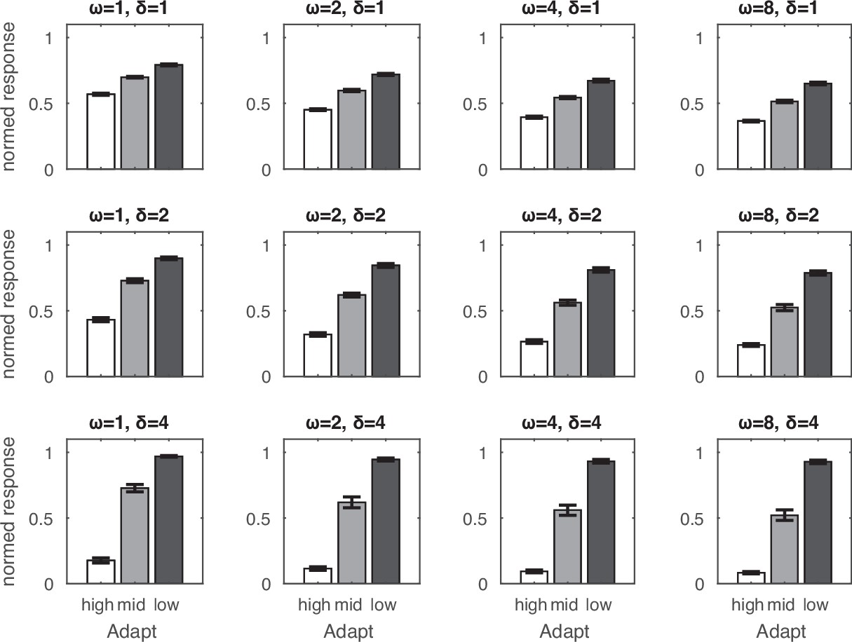
Adaptation effects as a function of model parameters.
In this simulation, the target of 10 dots was preceded by an adaptor of 5, 10, or 20 dots. Temporal normalization could be understood in terms of a sigmoid response curve with the amplification factor (δ) determining the slope of the curve and the recency weighting factor (ω) determining the horizontal position of the curve. Smaller ω values resulted in a relative overestimation of the normalized response to the target, which can be explained by the relative leftward horizontal shift of the sigmoid response curve and hence relative increase in normalized activity (nonlinearly as a function of driving input). Larger δ values resulted in greater under- and overestimation effects, which can be explained by the sharpening of the sigmoid response curve. Error bars indicate one standard deviation of the normalized response across 32 simulations.
Figure 3—figure supplement 4
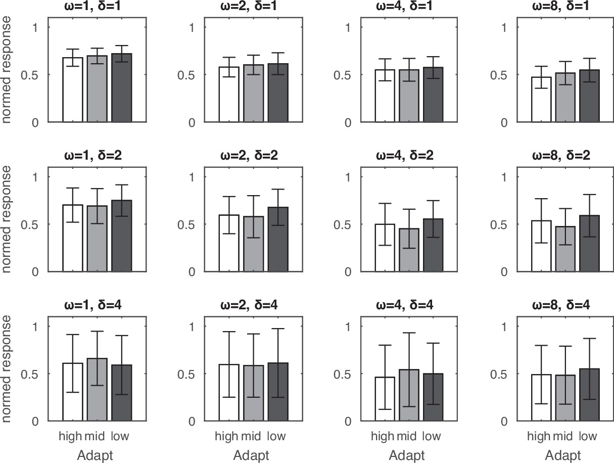
Adaptation effects along the size dimension.
The target of medium-sized array was preceded by an adaptor of small-, medium-, or large-sized array. No systematic pattern of adaptation was observed in these simulations. Error bars indicate one standard deviation of the normalized response across 32 simulations.
Figure 3—figure supplement 5
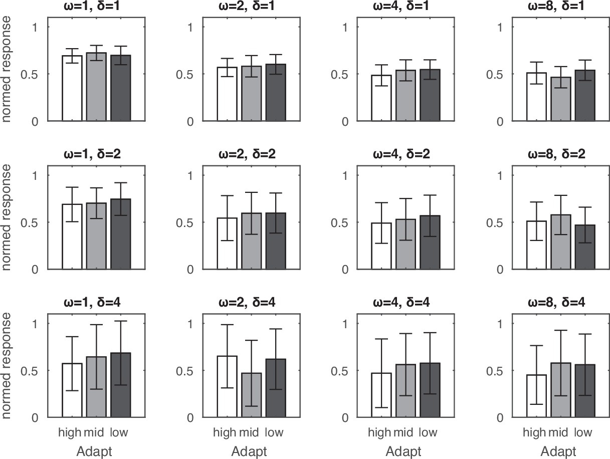
Adaptation effects along the spacing dimension.
The target of medium-spaced array was preceded by an adaptor of small-, medium-, or large-spaced array. No systematic pattern of adaptation was observed in these simulations. Error bars indicate one standard deviation of the normalized response across 32 simulations.
Figure 3—figure supplement 6
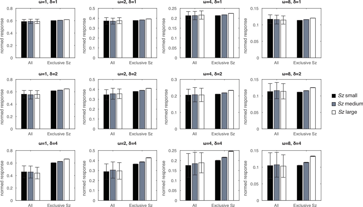
Context effects as a function of model parameters.
When the model saw 400 dot arrays that varied randomly across number, size, and spacing, the normalized responses to images corresponding to small, medium, and large sizes (Sz) showed no association with size. When then model saw 400 dot arrays that differed only in size, the normalized responses were strongly associated with size. Such a pattern was consistent across all the simulations over various amplification factors (δ) and recency weighting factors (ω) tested. Error bars represent one standard deviation of the normalized response across 128 simulations. Note that the error bars in the exclusive change in size conditions are extremely small.
Figure 3—figure supplement 7
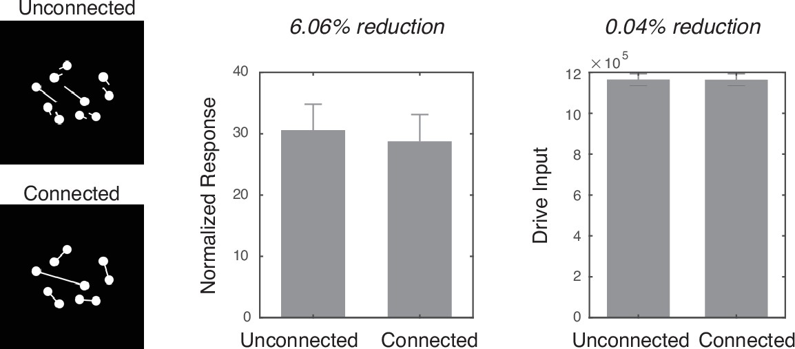
Simulation of the connectedness illusion.
In order to simulate the connectedness illusion, one set of ‘connected’ dot arrays and another set of ‘unconnected’ dot arrays were constructed. First, a large number of dot arrays with n=10, rd=6.5 pixels, and rf=64 pixels were created. Then, connected dot arrays were constructed by connecting the centers of two dots with a thin white line that was 2 pixels in width. The resulting images were visually checked, and all the images in which the lines cross or touch other lines or dots were removed from the set. Then, unconnected dot arrays were constructed from those connected dot arrays by breaking the midpoints of the interconnecting lines and rotating those broken lines about the center of each dot by ±30° in either direction randomly determined. The resulting images were checked again for any cross over of lines, in which case both that image and the corresponding connected image were removed. A total of 16 connected and 16 unconnected arrays entered the simulation. The connected arrays were underestimated by over 6% (Cohen’s d=5.72). Such an underestimation was not observed when considering the driving input (i.e., the model without divisive normalization). Error bars represent one standard deviation of the normalized response across simulations.
Figure 4
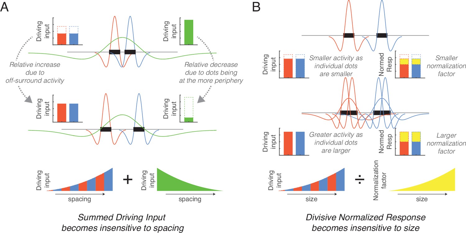
Simplified schematics explaining the mechanisms underlying the normalization of size and spacing.
(A) As spacing increases (from top to middle row) the response of small size center-surround filters increases (red and blue) whereas the response of large size center-surround filters decreases (green), with these effects counteracting each other in the total response. (B) As dot size increases (from top to middle row), more filters are involved in responding to the dots thereby increasing the unnormalized response (red and blue), but this results in a greater overlap in the neighborhoods and increases the normalization factor (yellow). These counteracting effects eliminate the size effect.
Tables
Table 1
Mathematical relationship between various magnitude dimensions.
| Dimension | As a function of n, rd, rf | As a function of N, Sz, Sp |
|---|---|---|
| Individual area (IA) | ||
| Total area (TA) | ||
| Field area (FA) | ||
| Sparsity (Spar) | ||
| Individual perimeter (IP) | ||
| Total perimeter (TP) | ||
| Coverage (Cov) | ||
| Closeness (Close) |
-
Note: n=number; rd=radius of individual dot; rf=radius of the invisible circular field in which the dots are drawn.
Additional files
Download links
A two-part list of links to download the article, or parts of the article, in various formats.
Downloads (link to download the article as PDF)
Open citations (links to open the citations from this article in various online reference manager services)
Cite this article (links to download the citations from this article in formats compatible with various reference manager tools)
A visual sense of number emerges from divisive normalization in a simple center-surround convolutional network
eLife 11:e80990.
https://doi.org/10.7554/eLife.80990


