Dynamics of immune memory and learning in bacterial communities
- Department of Physics, University of Toronto, Canada
- Institute of Biomaterials & Biomedical Engineering, University of Toronto, Canada
Figures
Figure 1 with 7 supplements
Model description.
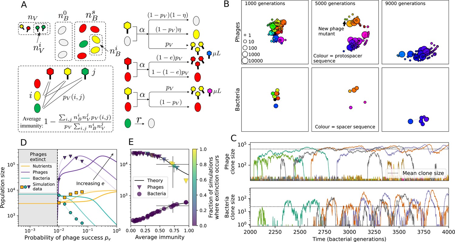
(A) We model bacteria and phages interacting in a well-mixed vessel. We track nutrient concentration, phage population size (), and bacteria population size (). Bacteria can either have no spacer () or a spacer of type (, ), and phages can have a single protospacer of type (). With rate , a phage interacts with a bacterium. If the bacterium does not have a matching spacer, the phage kills with probability and produces a burst of new phages, while for bacteria with a matching spacer that probability is reduced to , . Bacteria without spacers that survive an attack have a chance to acquire a spacer with probability , and bacteria with spacers lose them at rate . Lower inset: average immunity is the weighted average pairwise immunity between spacer-containing bacteria and phages, given by . The probability of a phage with protospacer successfully infecting a bacterium with spacer is . (B) Three time points in a typical simulation with , , , and . Coloured circles represent unique protospacer or spacer sequences; shared sequences are shown with the same colour. The size of each circle is proportional to clone size, and new mutants are shown radially more distant from the centre. (C) Ten individual clone trajectories vs simulation time for phages (top) and bacteria (bottom). The mean clone size is shown with a horizontal dashed line. (D) Total phage, bacteria, and nutrient concentration as a function of phage success probability . Markers show an average over five independent simulations for different values of with , and . Solid lines show theoretical predictions for different constant values of effective . As decreases, phages go extinct at a critical value given by , where . (E) Total phage and bacteria population size as a function of average bacterial immunity to phages. Colours indicate the fraction of simulations in which phage or bacteria go extinct before a set endpoint. Solid lines show the mean-field prediction. Error bars are the standard deviation across three or more independent simulations.
Figure 1—figure supplement 1

Probability of stochastic extinction at low spacer acquisition.
Probability of extinction in four or more simulations with the same parameters vs. mean phage population size (left) and mean bacteria population size (right) for the lowest value of spacer acquisition probability (). Colours indicate mutation rate and shapes indicate CRISPR effectiveness .
Figure 1—figure supplement 2
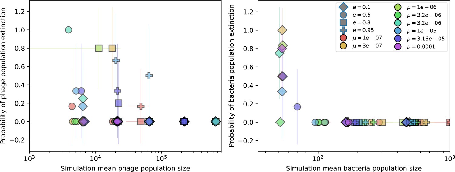
Probability of stochastic extinction at high spacer acquisition.
Probability of extinction in four or more simulations with the same parameters vs. mean phage population size (left) and mean bacteria population size (right) for the highest value of spacer acquisition probability (). Colours indicate mutation rate and shapes indicate CRISPR effectiveness . Error bars are the standard deviation across three or more independent simulations.
Figure 1—figure supplement 3

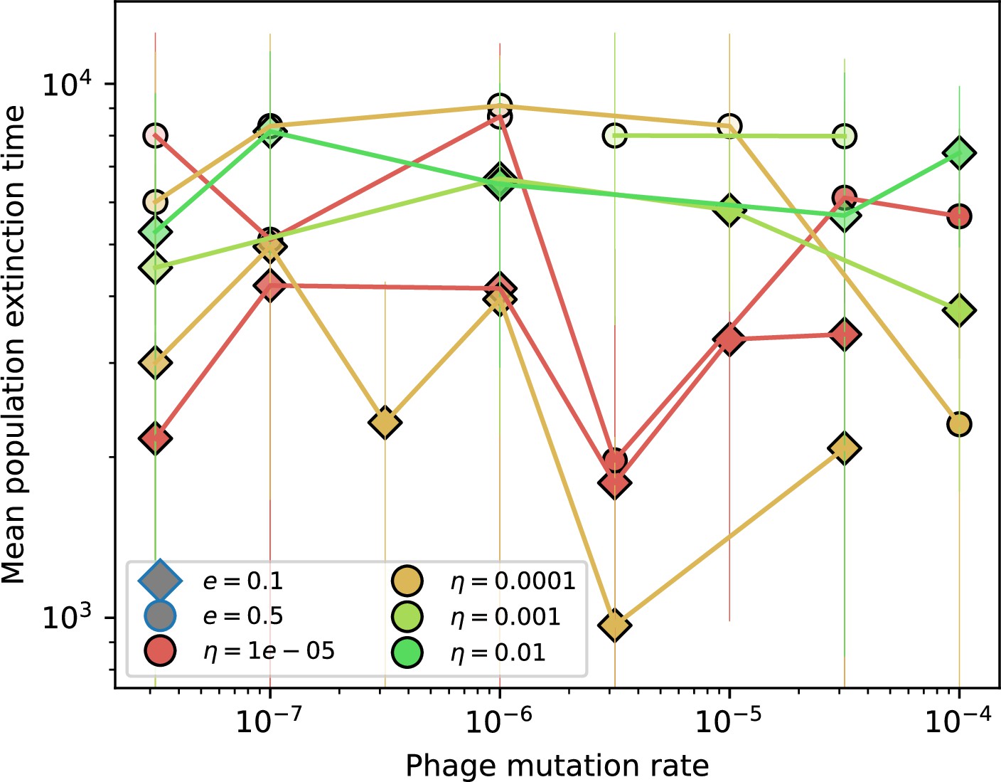
Time to extinction for phages vs. mutation rate.
Mean time for the phage population to go extinct vs. phage mutation rate across simulations where at least one simulation experienced phage extinction. The darkness of each point indicates the fraction of simulations that went extinct with darkest colours representing all simulations extinct. Simulations are shown for . Error bars are the standard deviation across three or more independent simulations.
Figure 1—figure supplement 4
Time to extinction for bacteria vs. mutation rate.
Mean time for the bacteria population to go extinct vs. phage mutation rate across simulations where at least one simulation experienced bacteria extinction. The darkness of each point indicates the fraction of simulations that went extinct with darkest colours representing all simulations extinct. Error bars are the standard deviation across three or more independent simulations.
Figure 1—figure supplement 5

Time to extinction for phages for different initial diversity and low spacer acquisition.
Mean time for the phage population to go extinct vs. phage mutation rate across simulations where at least one simulation experienced phage extinction. The darkness of each point indicates the fraction of simulations that went extinct with darkest colours representing all simulations extinct. Colours represent number of initial phage clones . Simulations are shown for and . Error bars are the standard deviation across three or more independent simulations.
Figure 1—figure supplement 6

Time to extinction for phages for different initial diversity and high spacer acquisition.
Mean time for the phage population to go extinct vs. phage mutation rate across simulations where at least one simulation experienced phage extinction. The darkness of each point indicates the fraction of simulations that went extinct with darkest colours representing all simulations extinct. Colours represent number of initial phage clones . Simulations are shown for and . Error bars are the standard deviation across three or more independent simulations.
Figure 1—video 1
An animation of a typical simulation of bacteria and phages interacting with CRISPR immunity.
Each bacteria can have a single spacer, indicated by colour, and each phage has a single protospacer sequence. Matching sequences are shown with the same colour. The size of each circle is proportional to clone size, and new mutants are shown radially more distant from the centre. New phages appear by mutation over time; many of them go extinct, but some establish and grow large, and then bacteria acquire matching spacers.
Figure 2 with 4 supplements
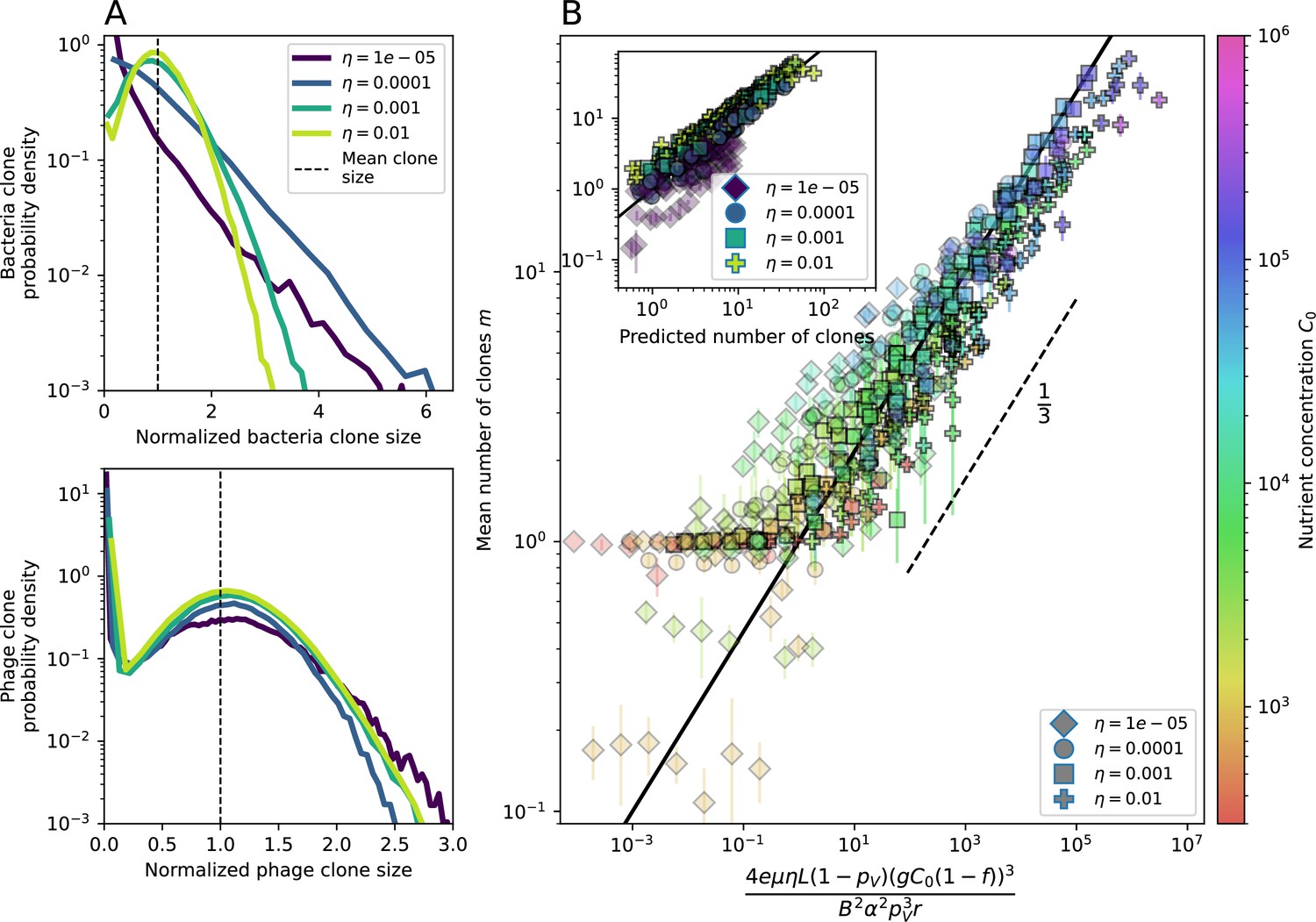
Diversity depends sub-linearly on parameters.
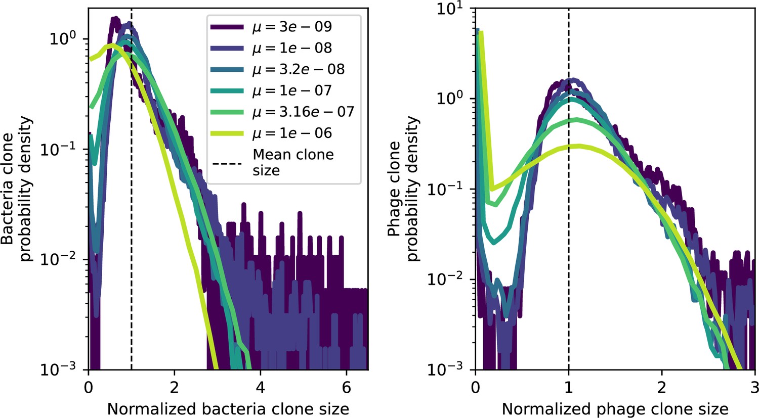
(A) Bacteria and phage clone size distributions normalized to the measured mean clone size for , , and . As increases, both clone size distributions become more sharply peaked. (B) The mean number of bacterial clones depends only on a combined parameter in the limit of small average immunity (generally coinciding with high C0). (Inset) The mean number of bacterial clones can be predicted by numerically solving Equation 1 for . The two lowest values of are shown with lighter shading. Error bars are the standard deviation across three or more independent simulations.
Figure 2—figure supplement 1
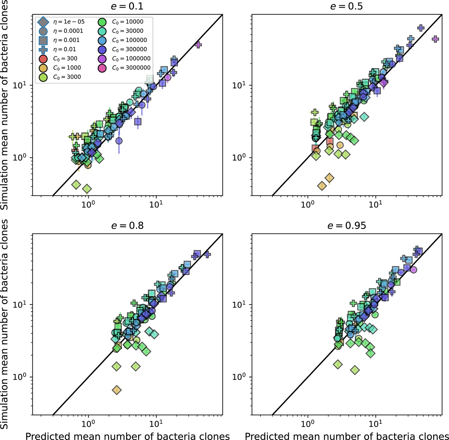
Predicted diversity grouped by spacer effectiveness.
Simulation mean number of bacteria clones () vs. theoretical prediction for given by numerically solving Equation 1, broken down by different values of . Error bars are the standard deviation across three or more independent simulations.
Figure 2—figure supplement 2
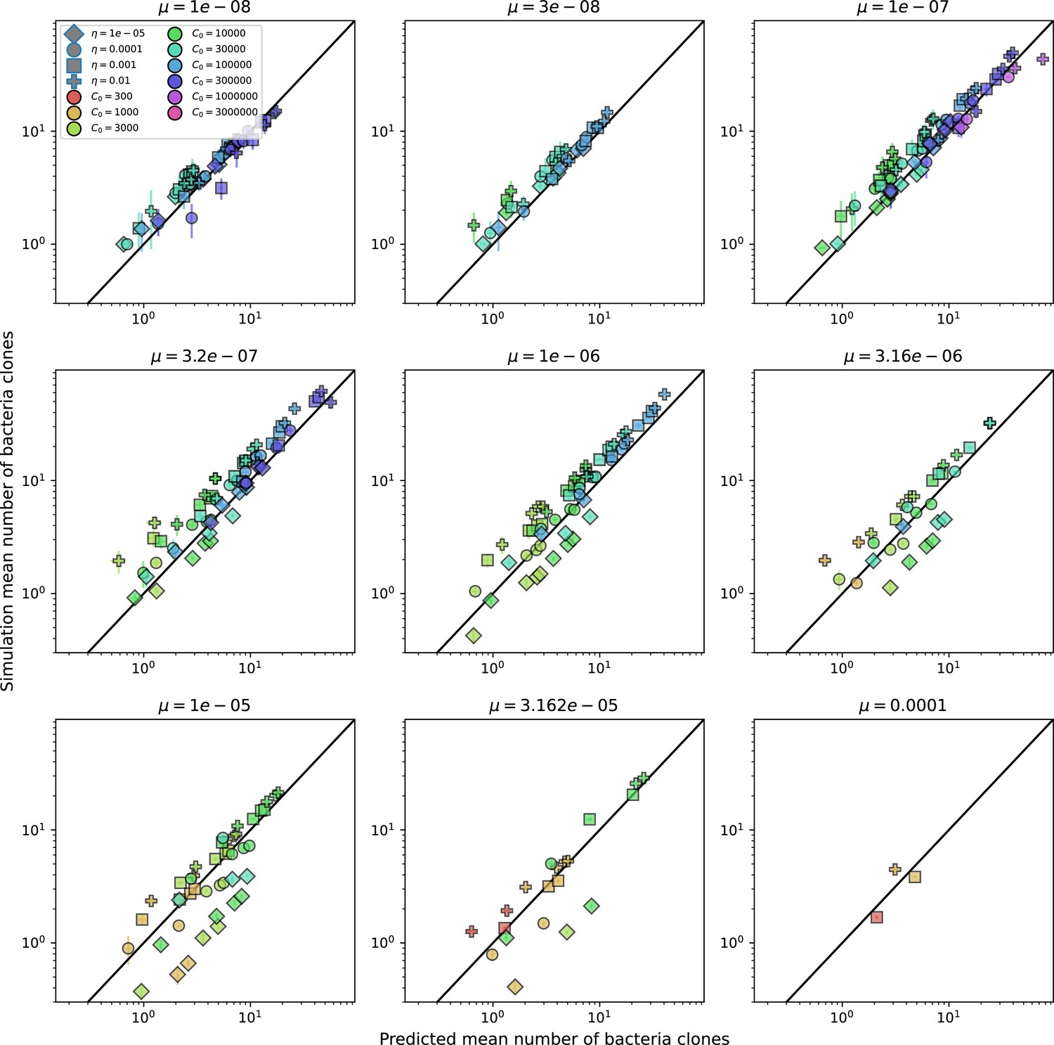
Predicted diversity grouped by mutation rate.
Simulation mean number of bacteria clones () vs. theoretical prediction for given by numerically solving Equation 1, broken down by different values of . Error bars are the standard deviation across three or more independent simulations.
Figure 2—figure supplement 3

Clone size histograms by spacer effectiveness.
Bacteria and phage clone size distributions normalized to the measured mean clone size for , , and .
Figure 2—figure supplement 4
Clone size histograms by phage mutation rate.
Bacteria and phage clone size distributions normalized to the measured mean clone size for , , and .
Figure 3 with 3 supplements
The fate of individual clones.
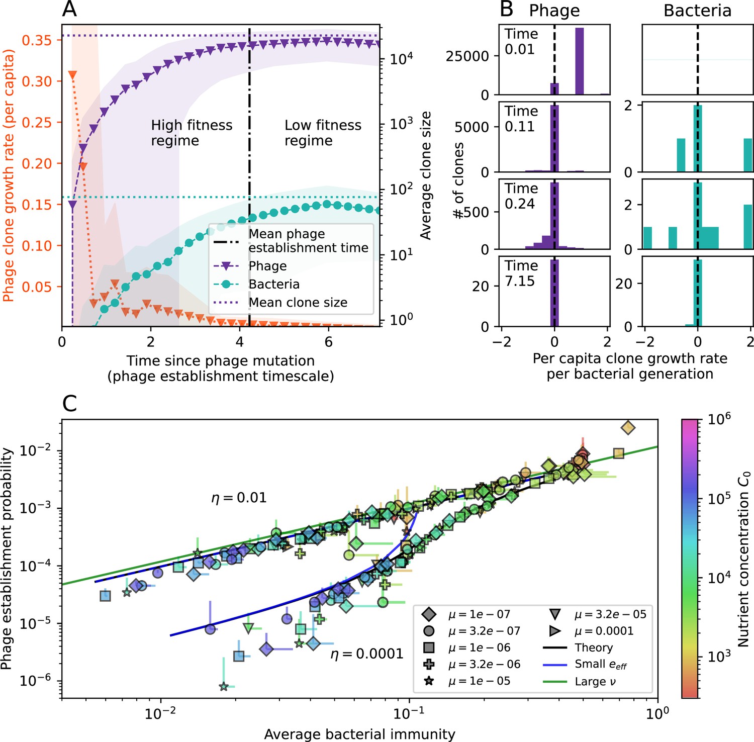
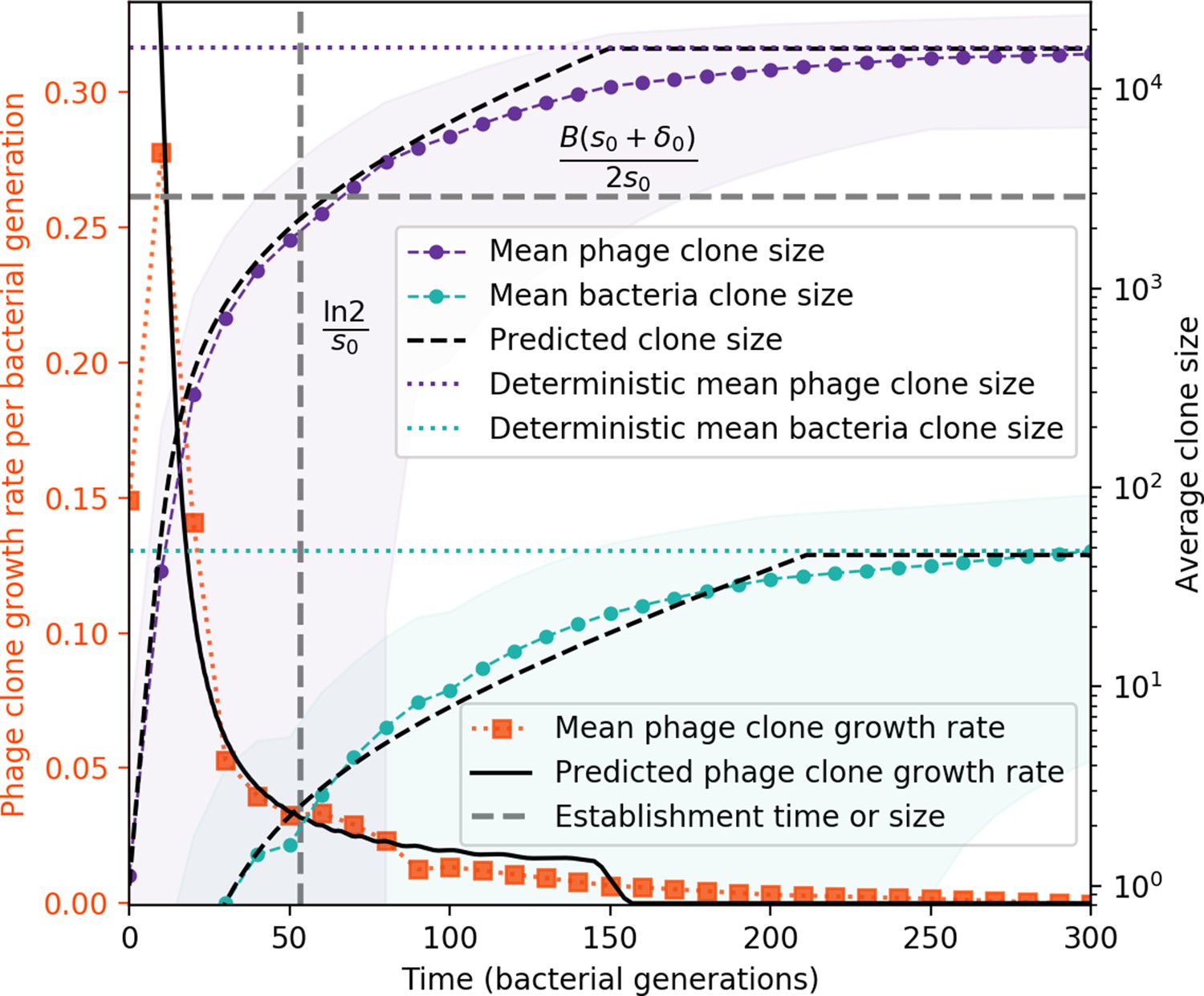
(A) Phage and bacteria coevolve in two timescale-separated regimes characterized by phage clone fitness. Average phage and bacteria clone size vs. time since phage mutation (right axis), and average clone growth rate vs. time since phage mutation (left axis). Markers show the average over all clone trajectories after steady state from six simulations with the same parameters. (B) Histograms of individual clone fitness grouped by time since phage mutation. Phage clones initially have fitness gt0, but rapidly most clones reach neutral growth (fitness ). Bacteria clones also follow suit, initially having fitness gt0 and rapidly reaching 0 fitness on average. Because spacer acquisition for a clone only happens after that clone is created by phage mutation, the top-right panel of (B) is empty at the earliest time point following phage mutation. Individual clone trajectories are highly variable. (C) Probability of phage clone establishment vs. average immunity. Clones are considered established in simulations when they reach the mean clone size. Equation 3 with is shown in green and with given by Equation 4 in blue. In (A, B), , , , and . Error bars are the standard deviation across three or more independent simulations.
Figure 3—figure supplement 1
Average clone sizes and fitness over time in a simulation.
Average phage and bacteria clone size vs. time (right vertical axis, purple and green markers) and average phage clone growth rate vs. time (left vertical axis, orange markers). Markers are the average over all clone trajectories after steady state in a single simulation. Phage clones appear at size 1 and grow until they reach the deterministic mean phage clone size on average. Once a phage clone becomes large, bacteria encounter it often enough to acquire a matching spacer, and bacteria clones grow until they reach their deterministic mean clone size. New phage mutants have a selective advantage (fitness gt0, positive growth rate) until they reach the deterministic mean clone size, at which point they evolve neutrally (fitness ). Individual clone trajectories are highly variable, leading to a large standard deviation on the mean phage clone fitness and a fitness trend which is only evident on average. The predicted clone size is piecewise-defined as the theoretical clone trajectory until the theoretical trajectory reaches the predicted mean clone size.
Figure 3—figure supplement 2

Approximations for phage establishment probability.
Phage establishment probability vs. effective . Markers are simulation results; error bars are standard deviation across three or more independent simulations. Black lines are the numerical theoretical solution. Blue lines are the approximate solution given by Equation 54 (with the full theoretical predicted value of ), and green lines are the same but with . All values of collapse on the same lines; the establishment probability depends only on and not on by itself. Interestingly, the approximation is close to the small approximation at high . This implies that high matters more at small . For some simulations near the transition from low to high , the probability of establishment is zero, which is why the grey connecting lines drop below the x-axis near effective .
Figure 3—figure supplement 3
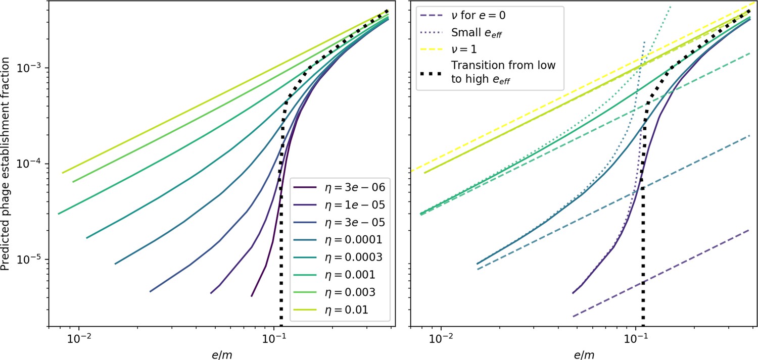
Theoretical phage establishment probability with approximations.
Theoretical phage establishment probability vs. . Solid lines are the numerical theoretical solution. Light dashed lines (‘small ’) are the approximate solution given by Equation 54 (with the full theoretical predicted value of ), heavy dashed lines are the same but with . All values of collapse on the same lines; the establishment probability depends only on and not on by itself. The inflection point in (dashed black line) is given by Equation 58.
Figure 4 with 4 supplements
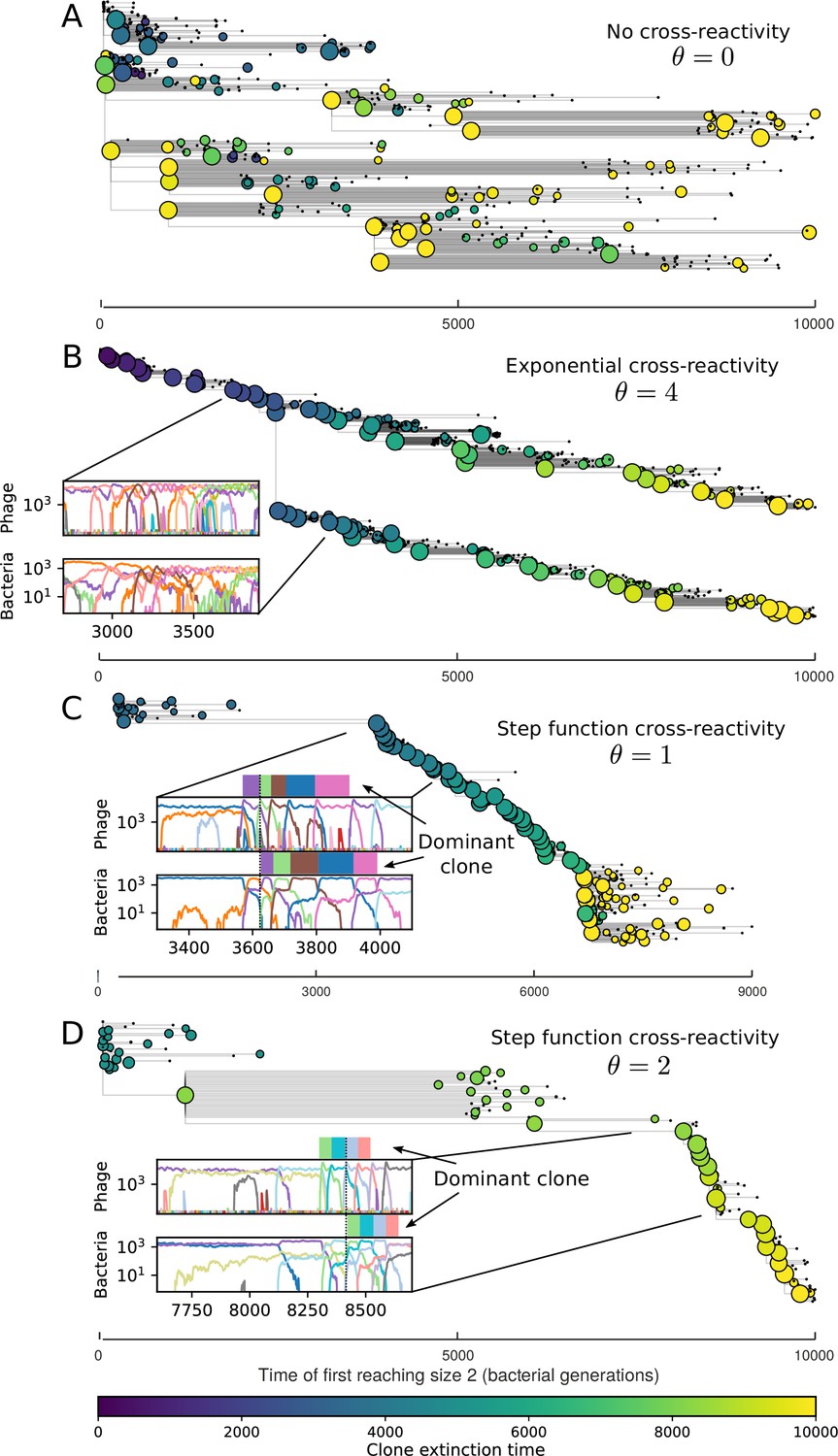
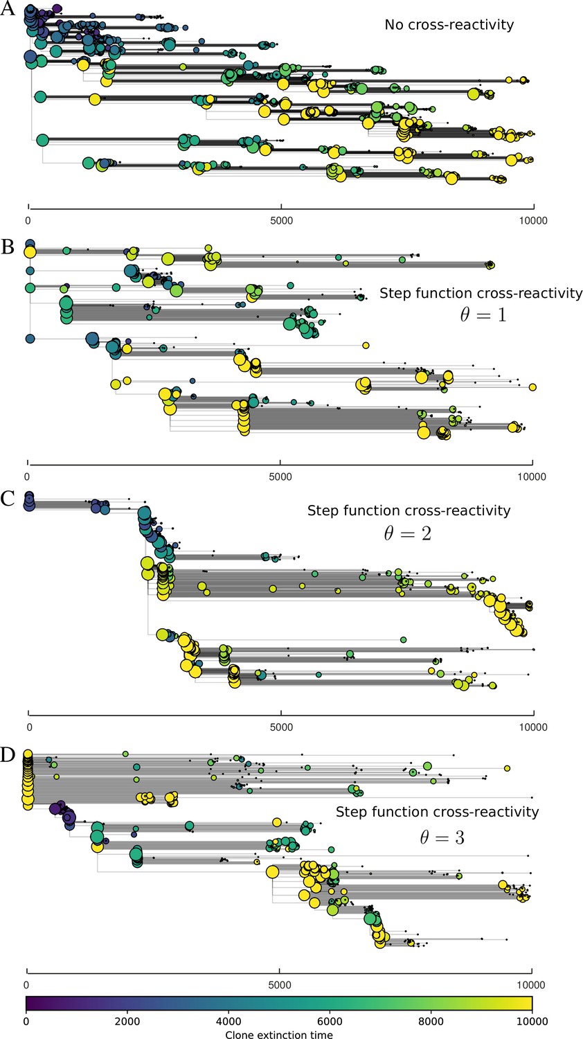
Cross-reactivity leads to ‘spindly’ phylogenies and regime switching.
Phage clone phylogenies for four simulations with different cross-reactivities: no cross-reactivity (A), exponential cross-reactivity with (B), and step-function cross-reactivity with (C) and (D). All simulations share all other parameters: . Phage clones are plotted at the first time they pass a population size of 2 to remove clutter from many new mutations destined for extinction, and the size of each circle is logarithmically proportional to the maximum size reached by that clone. Colours indicate the time of extinction of each clone. For each simulation with cross-reactivity, the left inset shows phage (top) and bacteria (bottom) clone sizes over time; colours indicate unique clone identities. Coloured rectangles above insets in (C) and (D) correspond to the dominant clone at each time. Dominant clone identities are offset by (vertical dashed line for visual aid).
Figure 4—video 1
Animation of simulation without cross-reactivity for Figure 4A.
Figure 4—video 2
Simulation animation with exponential cross-reactivity for Figure 4B.
Figure 4—video 3
Simulation animation with step-function cross-reactivity for Figure 4C.
Figure 4—video 4
Simulation animation with step-function cross-reactivity for Figure 4D.
Figure 5 with 1 supplement
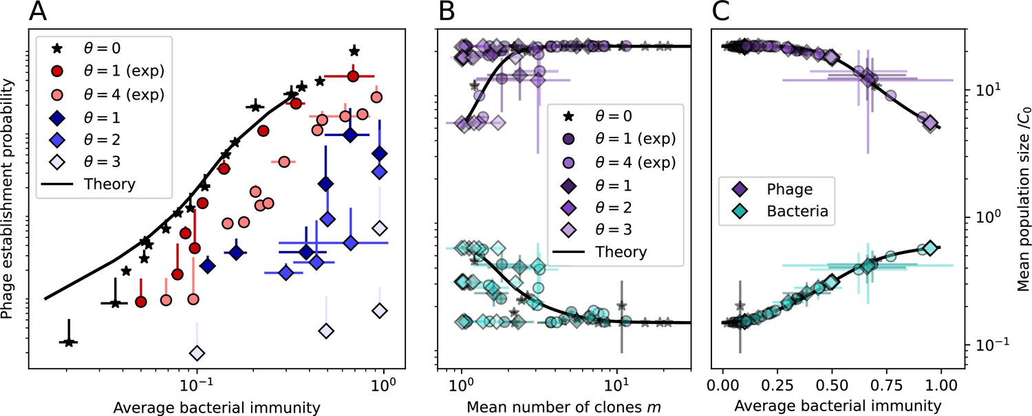
Average immunity underlies population outcomes.
(A) Probability of phage clone establishment vs. average immunity for different amounts and types of cross-reactivity. No cross-reactivity () is shown as black stars, exponential cross-reactivity in red, and step-function cross-reactivity in blue. Simulation averages are shown for and . Error bars are the standard deviation across three or more independent simulations and are shown in both x directions and the positive y direction. (B, C) Total phage (purple) and total bacteria (teal) average population sizes vs. the mean number of bacterial clones (B) and vs. average bacterial immunity (C) for . Each point is an average at steady state over three or more independent simulations with the same parameters; error bars are standard deviation. Total sizes are scaled by the initial nutrient concentration C0. Lighter colours indicate stronger cross-reactivity, marker shapes match legends in (A) and (B). Solid lines are the predicted total population size given by solving Equations 13–17 and using the approximation effective in (B) and the measured average immunity for effective in (C).
Figure 5—figure supplement 1

Total population sizes predicted by average immunity in a simulation with cross-reactivity.
Total phage (top) and total bacteria (bottom) in a simulation with cross-reactivity (step function CRISPR effectiveness with ). The dashed black line uses the measured value of average immunity from the simulation at each time point to predict population sizes using the solutions to the system of Equations 13–17. This simulation has one initial phage clone and parameters , , , and .
Figure 6 with 5 supplements
Phage evolution and spacer turnover.
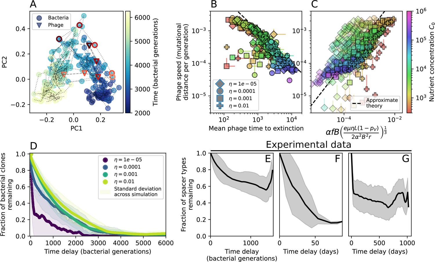
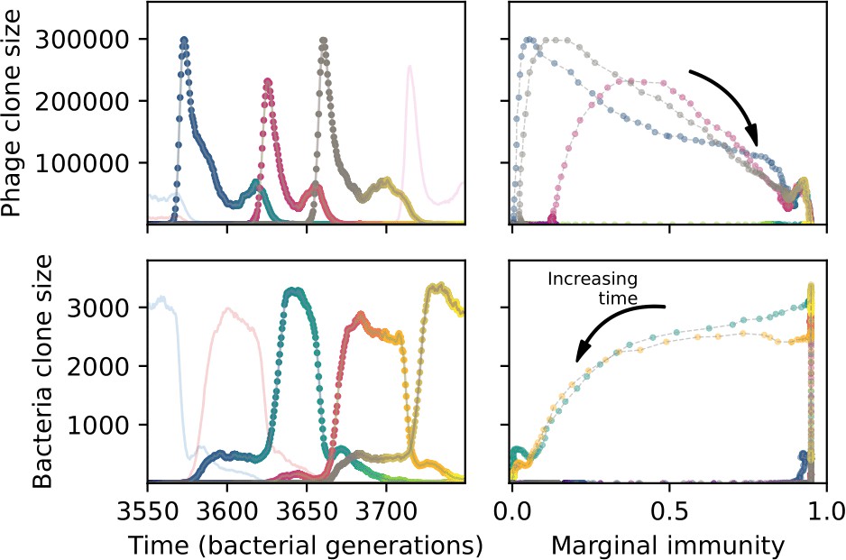
(A) Principal Component Analysis (PCA) decomposition of phage and bacteria clone abundances for a simulation with , , , and . Clone abundances are normalized at each time point, then PCA is performed for the entire phage time series over generations (four times the mean extinction time for phage clones). Bacteria and phage clone abundances are transformed into the PCA coordinates; colours indicate simulation time. Five time points are highlighted in progressively lighter shades of red for emphasis. (B) Phage genomic speed of evolution vs. mean large phage clone time to extinction. The phage speed is the weighted average genomic distance between the phage population at the end of the simulation and the phage population at an earlier time, divided by the time interval. The dashed line is . (C) The speed of evolution increases as spacer effectiveness , spacer acquisition probability , and phage mutation rate increase. The dashed line shows an approximate theoretical calculation (assuming speed = 1/time to extinction) which captures the trend across a wide range of parameters. Error bars in (B) and (C) are the standard deviation across three or more independent simulations and are shown in the positive direction only. (D) Spacer turnover as a function of time delay for four simulations with , , and . The fraction of bacterial clones remaining is the fraction of clones that were present at time that are still present at time delay. Solid lines are an average across steady-state for each value of the time delay; shaded regions are the standard deviation. (E–G) Spacer-type turnover calculated as in (D) using experimental data from Paez-Espino et al., 2015 (E), metagenomic data sampled from groundwater from Burstein et al., 2016 (F), and metagenomic data sampled from a wastewater treatment plant from Guerrero et al., 2021a (G). Experimental time points are interpolated to the minimum sampling interval to allow averaging across the experiment.
Figure 6—figure supplement 1

Clone size PCA for a simulation with exponential cross-reactivity.
PCA decomposition of phage and bacteria clone abundances for a simulation with exponential cross-reactivity and , ,, and. Clone abundances are normalized at each time point, then PCA is performed for the entire phage time series over generations (four times the mean extinction time for phage clones). Bacteria and phage clone abundances are transformed into the PCA coordinates; colours indicate simulation time. Five time points are highlighted in progressively lighter shades of red for emphasis.
Figure 6—figure supplement 2
Genetic distance vs. diversity and time to extinction.
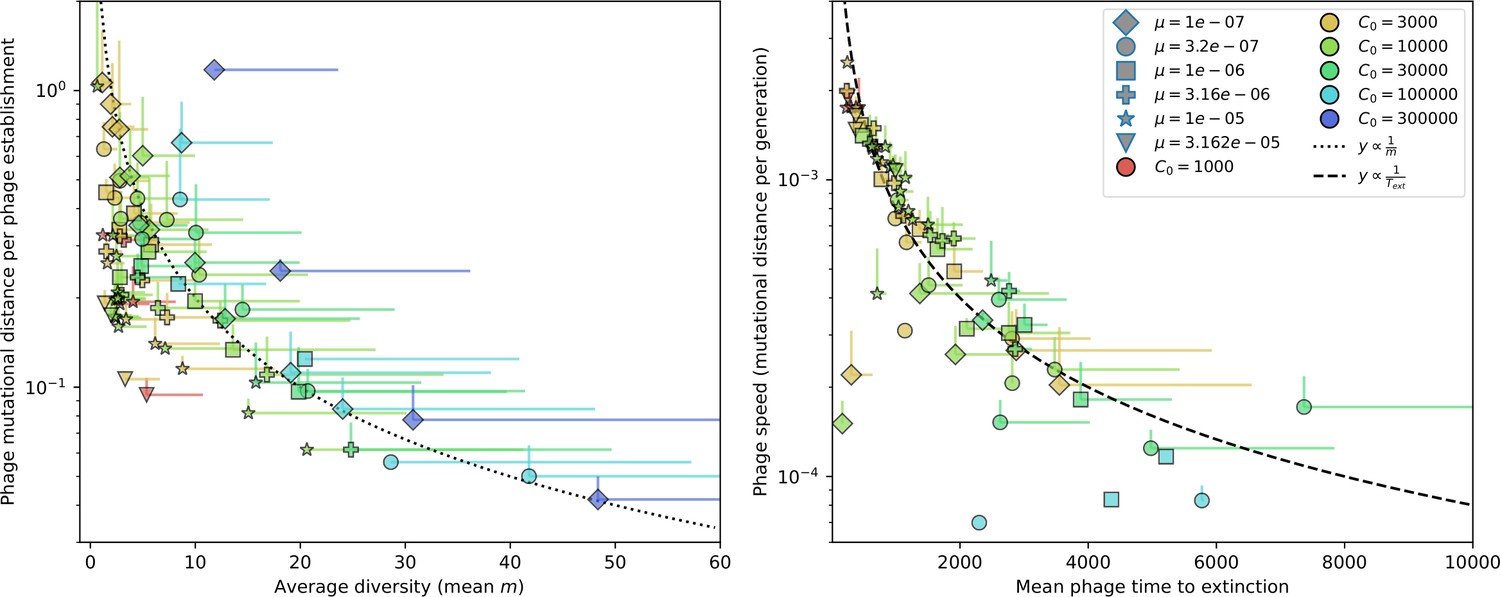
Phage mutational distance reached in simulations divided by the number of phage establishments vs. diversity (left) and phage mutational distance per generation vs. mean phage time to extinction (right). Error bars are the standard deviation across three or more independent simulations and are shown in the positive direction only.
Figure 6—figure supplement 3

Spacer turnover by spacer effectiveness.
Spacer turnover as a function of time delay for four simulations with , , and . The fraction of bacterial clones remaining is the fraction of clones that were present at time that are still present at time delay. Solid lines are an average across steady state for each value of the time delay; shaded regions are the standard deviation.
Figure 6—figure supplement 4

Spacer turnover by phage mutation rate.
Spacer turnover as a function of time delay for four simulations with , , and . The fraction of bacterial clones remaining is the fraction of clones that were present at time that are still present at time delay. Solid lines are an average across steady state for each value of the time delay; shaded regions are the standard deviation.
Figure 6—video 1
PCA decomposition of phage and bacteria protospacer and spacer clone abundances for a simulation of bacteria and phages interacting with CRISPR immunity.
Clone abundances are normalized at each time point, then PCA is performed for the entire phage time series over about 4000 generations (four times the mean extinction time for phage clones). Bacteria and phage clone abundances are transformed into the PCA coordinates; colours indicate simulation time.
Figure 7 with 12 supplements
Quantifying immune memory in data.
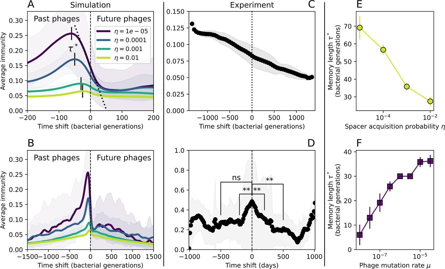
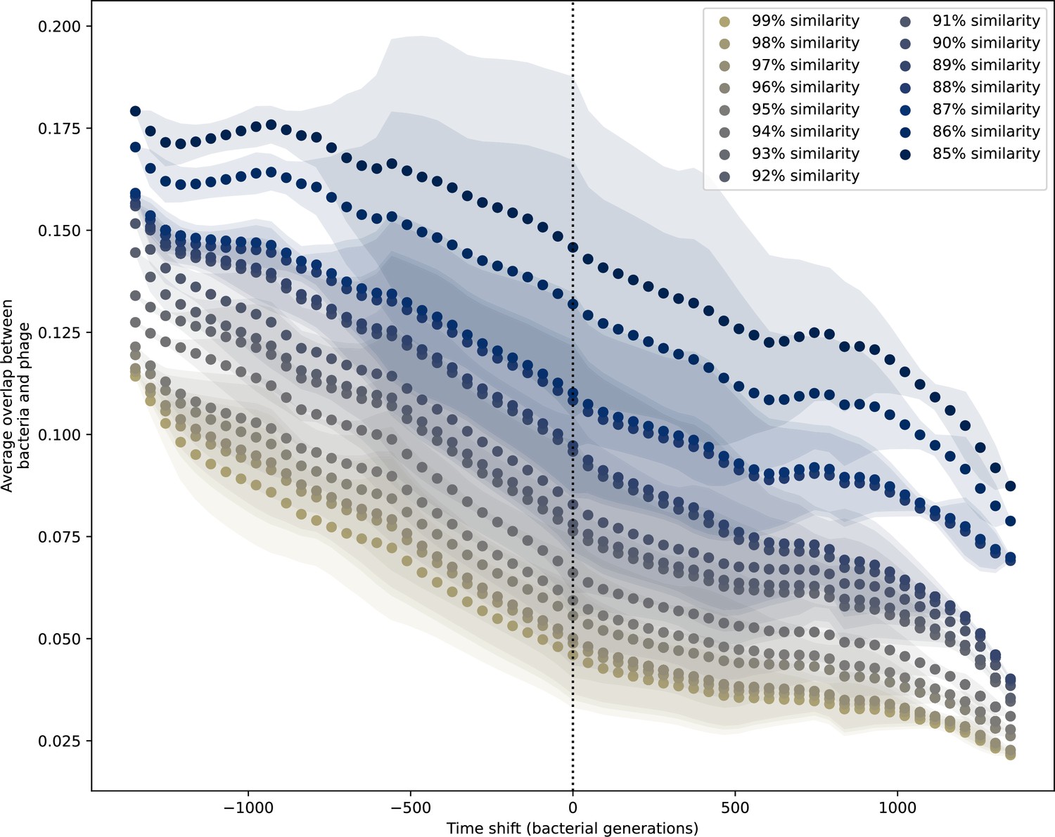
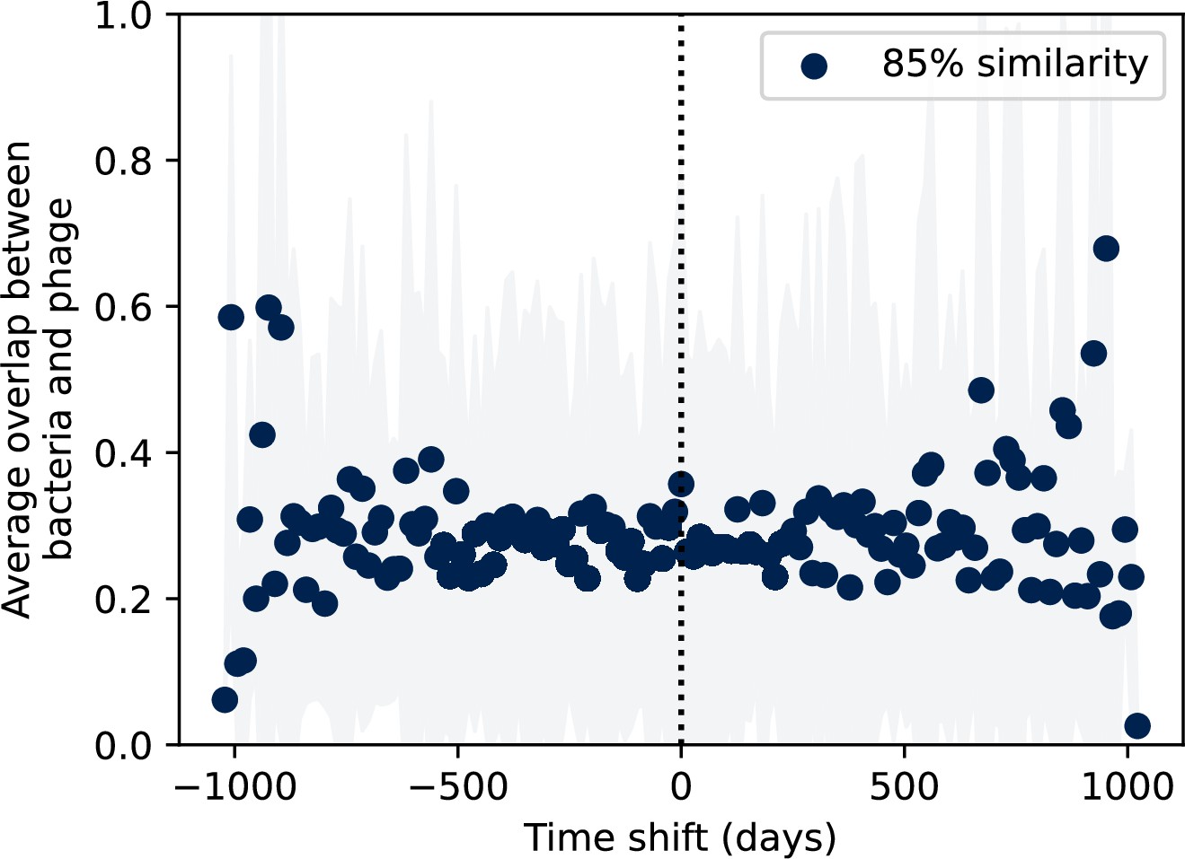
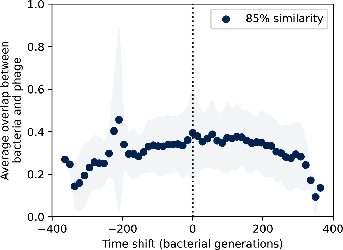
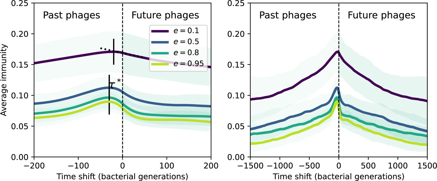
(A, B) Average immunity of bacteria against phage for four simulations with different values of as a function of time shift. Solid lines are an average across steady state for each value of the time shift; shaded regions are the standard deviation. Average immunity peaks in the recent past (A, indicated by ) with a negative slope through zero delay (A, black dashed line) and decays to zero at long delays in the past or future (B). For all simulations , , and . (C, D) Average overlap between bacterial spacer and phage protospacer types using data from a lab experiment with S. thermophilus and phage from Paez-Espino et al., 2015 (C) and data from a wastewater treatment plant sampled over 3 years from Guerrero et al., 2021a (D). Spacer types are grouped by 85% similarity, and shaded region is standard deviation across averaged data. Base average immunity values were multiplied by the average number of protospacers corresponding to the S. thermophilus CRISPR system (C) and the Gordonia CRISPR systems (D) to account for multiple potential protospacer targets per phage. In (D), we compared two time shifts with zero delay average immunity using a Wilcoxon signed-rank test: for lower past immunity at 500 days, for lower past immunity at 200 days, for lower future immunity at 500 days, and for lower future immunity at 200 days. (E, F) The position of the peak in past immunity for simulated data vs. spacer acquisition probability (E) and phage mutation rate (F). The peak position is the time shift value for which the curves in (A) are largest, indicated by . Error bars are the standard deviation across three or more independent simulations.
Figure 7—figure supplement 1
Time-shifted average immunity for experimental coevolution data.
Time shifted overlap for experimental coevolution data with the first time point and last two time points removed. Interpolation spacing is 3 days, the smallest interval between remaining time points. Time intervals in days were multiplied by 6.64, the estimated number of bacterial generations per day assuming exponential growth with 100:1 serial dilutions. Protospacers are included if they have a perfect PAM, and all wild-type spacers are included.
Figure 7—figure supplement 2
Time-shifted average immunity for experimental coevolution data with partial PAM matches included.
Time-shifted overlap for experimental coevolution data with the first time point and last two time points removed. Interpolation spacing is 3 days, the smallest interval between remaining time points. Time intervals in days were multiplied by 6.64, the estimated number of bacterial generations per day assuming exponential growth with 100:1 serial dilutions. Protospacers are included if they have a perfect PAM or partially perfect PAM, and all wild-type spacers are included.
Figure 7—figure supplement 3
Time-shifted average immunity for experimental coevolution data with all sequences regardless of PAM.
Time-shifted overlap for experimental coevolution data with the first time point and last two time points removed. Interpolation spacing is 3 days, the smallest interval between remaining time points. Time intervals in days were multiplied by 6.64, the estimated number of bacterial generations per day assuming exponential growth with 100:1 serial dilutions. All potential protospacers are included regardless of PAM sequence, and all wild-type spacers are included.
Figure 7—figure supplement 4
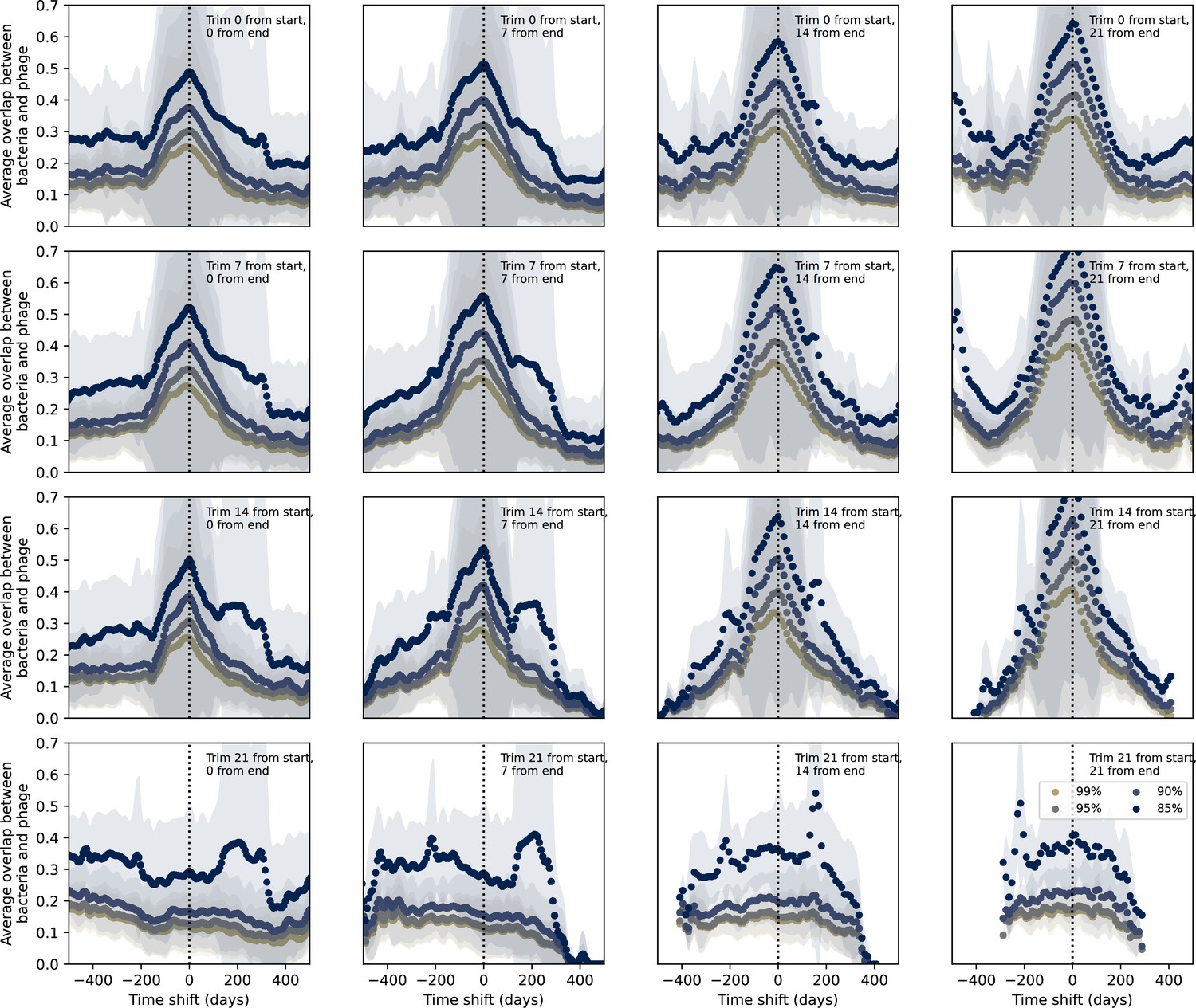
Time-shifted average immunity for experimental coevolution data with data trimmed from start and end.
Time-shifted overlap for experimental coevolution data with increasing numbers of time points from the start and end removed. Interpolation spacing is the smallest interval between remaining time points. Only perfect-PAM protospacers are included; all wild-type spacers are included.
Figure 7—figure supplement 5
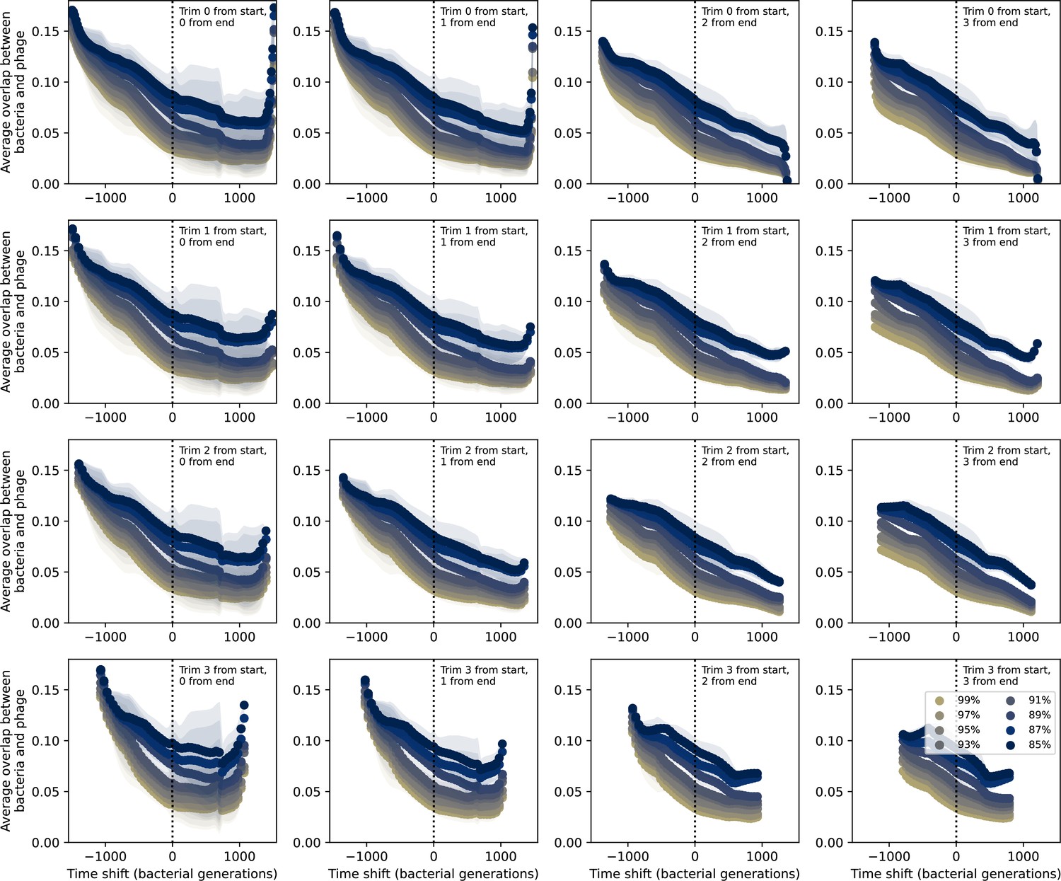
Time-shifted average immunity for wastewater with data trimmed from start and end.
Time-shifted average immunity for spacers and protospacers from wastewater grouped at four different similarity thresholds. Points are trimmed from the start and end of the time series in each panel as described in the overlay text. Raw values are multiplied by 1956, the average number of protospacers with the GTT PAM from the phage DC-56 and DS-92 genomes. Only perfect-PAM protospacers are included; all wild-type spacers are included.
Figure 7—figure supplement 6
Bootstrapped average immunity with all points randomly shuffled.
Bootstrapped control: time-shifted average immunity for wastewater after randomly shuffling the interpolated clone abundances separately for bacteria and phage.
Figure 7—figure supplement 7

Bootstrapped average immunity with pairs of bacteria and phage clone sizes shuffled.
Bootstrapped control: time-shifted average immunity for wastewater after randomly shuffling pairs of interpolated bacteria and phage clone sizes such that time point matching is maintained between bacteria and phages.
Figure 7—figure supplement 8

Time-shifted average immunity for wastewater with data trimmed from the end.
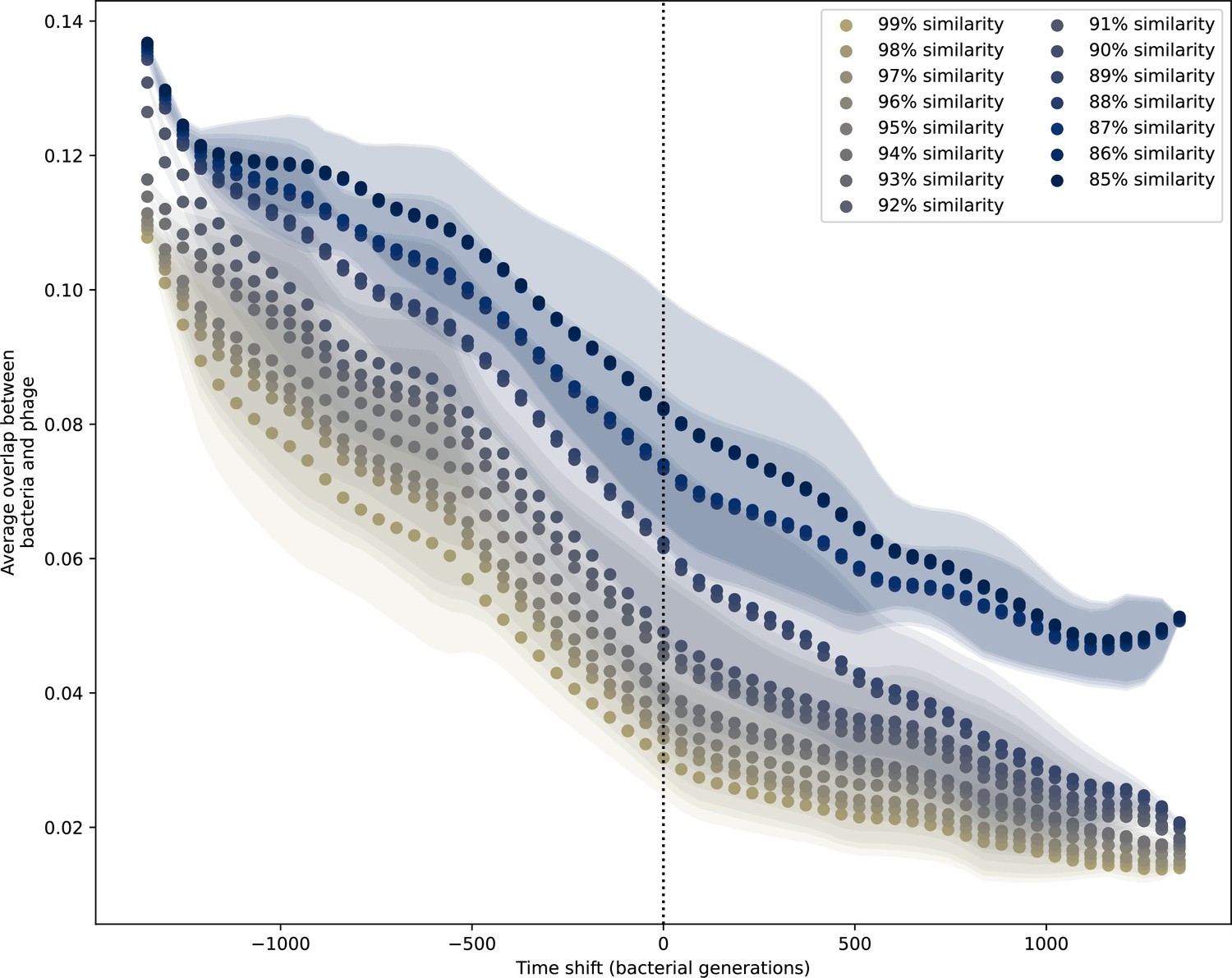
Time-shifted average immunity for spacers and protospacers grouped at an 85% similarity threshold. 16 time points are removed from the end of the data series in order to remove the region with zero protospacer counts. Raw values are multiplied by 1956, the average number of protospacers with the GTT PAM from the phage DC-56 and DS-92 genomes. Only perfect-PAM protospacers are included; all wild-type spacers are included.
Figure 7—figure supplement 9

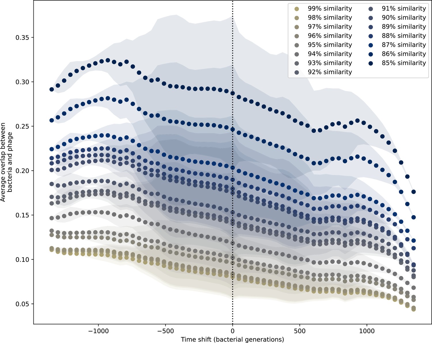
Time-shifted average immunity for wastewater with data trimmed from the start.
Time-shifted average immunity for spacers and protospacers grouped at an 85% similarity threshold. 21 time points are removed from the beginning of the data series to remove the region with anomalously high average immunity. Raw values are multiplied by 1956, the average number of protospacers with the GTT PAM from the phage DC-56 and DS-92 genomes. Only perfect-PAM protospacers are included; all wild-type spacers are included.
Figure 7—figure supplement 10
Time-shifted average immunity for wastewater with data trimmed from the start and end.
Time-shifted average immunity for spacers and protospacers grouped at an 85% similarity threshold. 21 time points are removed from the beginning of the data series to remove the region with anomalously high average immunity, and 16 time points are removed from the end of the data series in order to remove the region with zero protospacer counts. Raw values are multiplied by 1956, the average number of protospacers with the GTT PAM from the phage DC-56 and DS-92 genomes. Only perfect-PAM protospacers are included; all wild-type spacers are included.
Figure 7—figure supplement 11
Time-shifted average immunity by spacer effectiveness.
Average immunity of bacteria against phage for four simulations with different values of as a function of time shift. Solid lines are an average across steady-state for each value of the time shift; shaded regions are the standard deviation. A short-time view is shown on the left and a long-time view on the right. For all simulations , , and .
Figure 7—figure supplement 12

Time-shifted average immunity by phage mutation rate.
Average immunity of bacteria against phage for four simulations with different values of as a function of time shift. Solid lines are an average across steady state for each value of the time shift; shaded regions are the standard deviation. A short-time view is shown on the left and a long-time view on the right. For all simulations , , and .
Figure 8
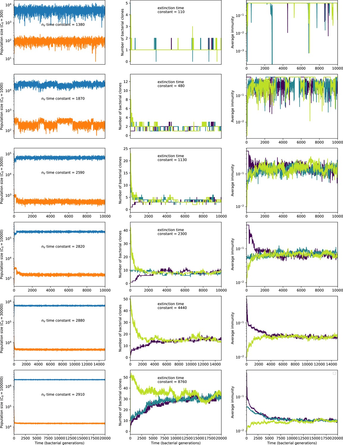
Total phage, total bacteria (left), and mean number of bacterial clones (right) vs. simulation time for five simulations with , , , and C0 ranging from 300 (top row) to 30,000 (bottom row).
Total population sizes equilibrate very quickly, but the total number of clones can take longer at large population sizes (high C0). The time constants inset are a measure of how quickly we expect each mean-field quantity to equilibrate: time constant is the inverse growth rate of the total phage population () and the extinction time constant is the mean time to extinction for large phage clones (Equation 171), a measure of the rate of turnover of the number of clones.
Figure 9

Mean number of bacterial clones after bacterial generations vs. initial number of phage clones for , .
The mean is an average of 15 evenly spaced points from to bacterial generations. Error bars are the standard deviation across three or more independent simulations.
Figure 10
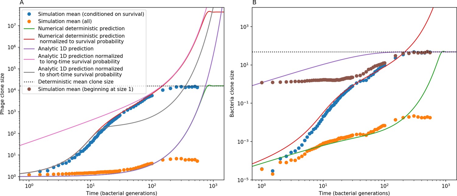
Phage (A) and bacteria (B) mean clone size in a simulation, either conditioned on survival (blue circles) or including extinct clones (orange circles).
Theoretical predictions are plotted as solid lines: the time-dependent numerical solution to Equations 21 and 22 in green, the same solution divided by the phage clone probability of survival in red, and a one-dimensional solution to Equation 21 in (A) and 22 in (B). Equations 25 and 26 are black dashed lines. An alternate simulation mean clone size is plotted for bacteria (brown circles) in which each clone trajectory is stacked based on the bacterial acquisition time and averaged across trajectories, conditioned on survival. Simulation parameters are , , , and .
Figure 11
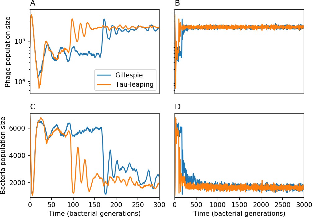
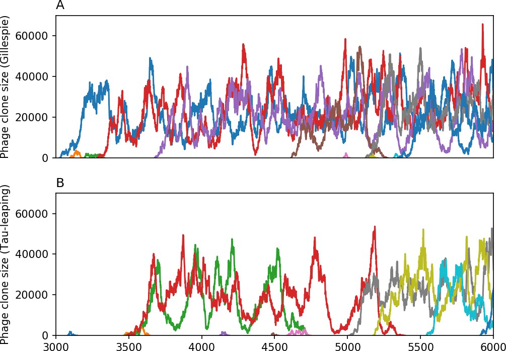
Total phage () and total bacteria () as a function of time for a Gillespie simulation and a tau-leaping simulation with the same parameters.
Total phage is shown at early times (A) and late times (B), and total bacteria at early times (C) and late times (D). The simulation parameters are , , , and . Early time dynamics differ slightly in this example, but the long-time behaviour and steady-state values are similar.
Figure 12
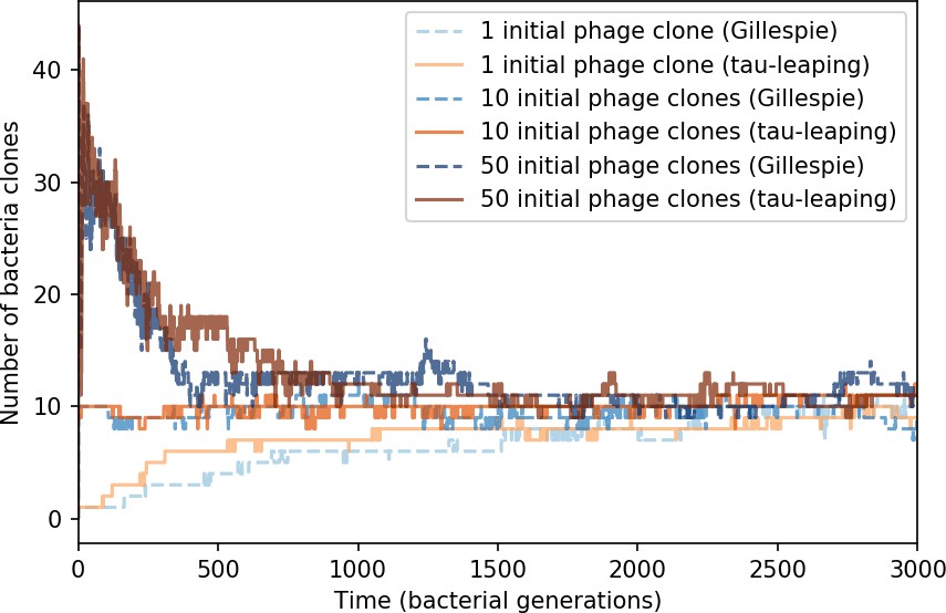
Number of bacterial clones () vs. simulation time for three sets of simulations, each beginning with 1, 10, or 50 phage clones.
Gillespie simulations are dashed blue lines, and tau-leaping simulations are solid orange and red lines. The simulation parameters are , , , and .
Figure 13
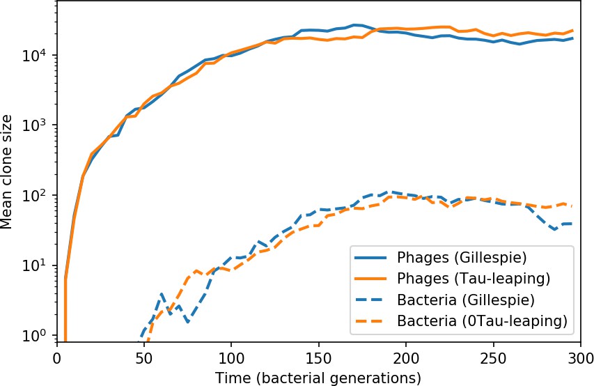
Average population size of phage clones (solid lines) and bacterial clones (dashed lines) in a Gillespie and tau-leaping simulation with the same parameters.
The simulation parameters are , , , and .
Figure 14
10 spacer trajectories for a Gillespie simulation (A) and tau-leaping simulation (B).
The first 10 trajectories that surpass are shown. The simulation parameters are , , , and .
Figure 15
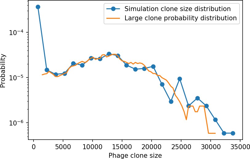
Phage clone size distribution from 15 combined time points for a simulation with the parameters , , , and .
The blue points are the values of the full normalized phage clone size histogram with a bin width of 1500. The orange line is given by in Equation 28 smoothed with a running average of window size 3000. Both distributions are scaled by the total number of phage clones.
Figure 16
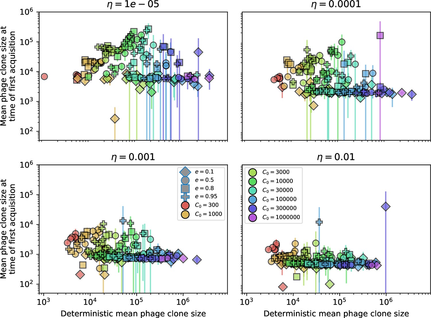
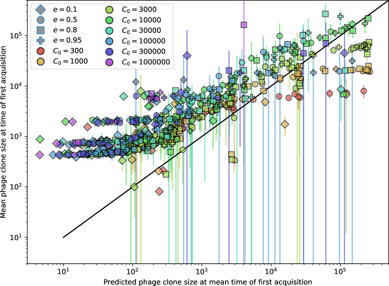
Mean phage clone size at the time of first spacer acquisition vs. the deterministic mean phage clone size.
For each phage clone trajectory, the clone size at the time of first spacer acquisition is recorded and these are averaged across each simulation. Error bars are the standard deviation across three or more independent simulations.
Figure 17
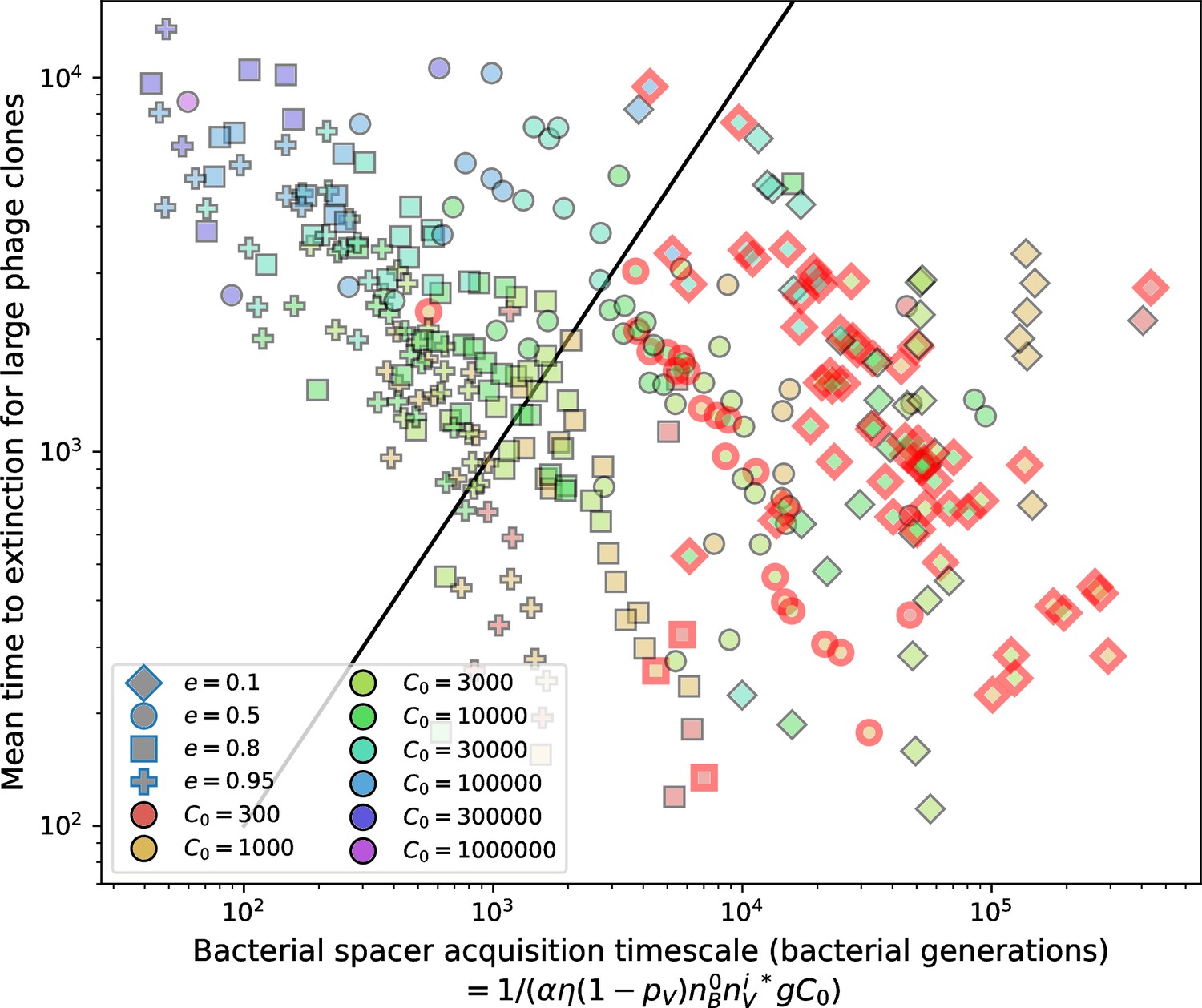
Mean time to extinction for phage clones vs. the timescale of bacteria spacer acquisition given by where .
Points outlined in red are simulations where the ratio of large phage clones to bacterial clones exceeds 1.2. Phage clones experience clonal interference at low : they go extinct faster than bacteria acquire spacers.
Figure 18
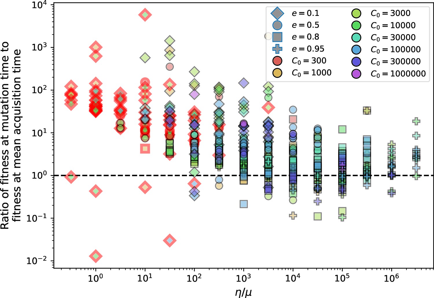
Ratio of average phage clone initial fitness to the average phage clone fitness at the mean bacterial spacer acquisition time vs .
Points outlined in red are simulations where the ratio of large phage clones to bacterial clones exceeds 1.2. The phage fitness is the average per capita growth rate of phage clones conditioned on survival. Phage clones experience clonal interference at low and high .
Figure 19
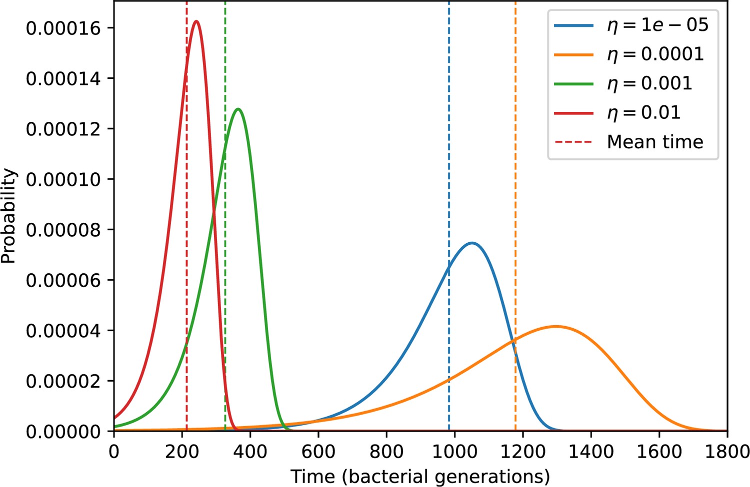
Probability of the first spacer acquisition happening at time for four simulations with different values of and , and .
The mean of each distribution is shown as a vertical dashed line.
Figure 20

Mean phage clone size at time of first spacer acquisition for simulation data, the predicted with Equation 31, and the prediction with the mode of the distribution given by Equation 29 for four simulations with different values of and , and .
Figure 21
Measured mean phage clone size at the time of first spacer acquisition vs. the prediction given by of Equation 31.
Error bars are the standard deviation across three or more independent simulations.
Figure 22
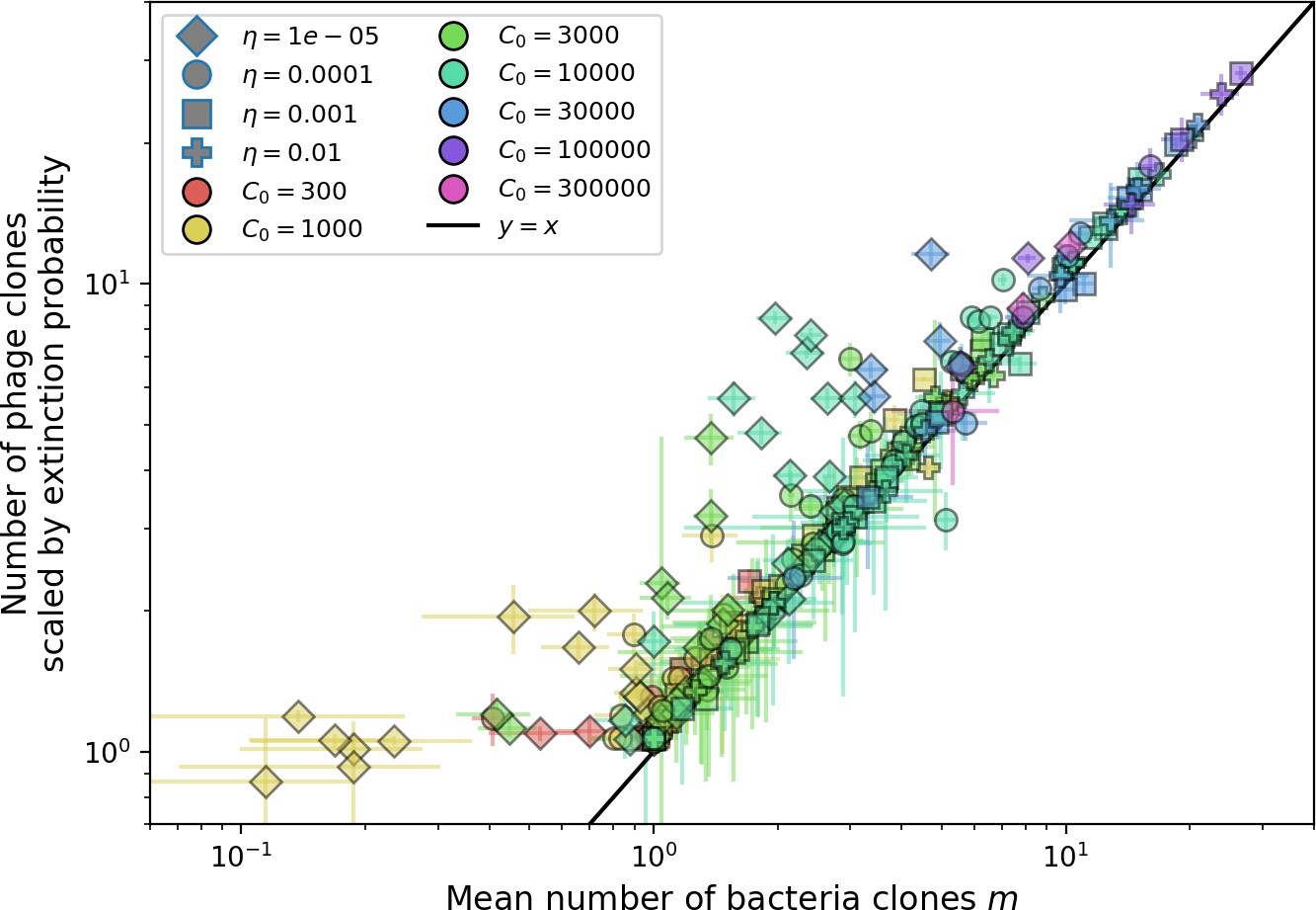
Mean number of large phage clones vs. mean number of bacterial clones in simulations.
For each simulation, we take a subset of 15 evenly spaced timepoints at steady state and calculate the size and number of phage clones present. We scale the observed clone sized distribution with Equation 28 and calculate the mean number of large phage clones by multiplying the total number of clones with the fraction of large phage clones given by . We use the simulation mean total population sizes to calculate s0 and in Equation 27. We obtain the mean number of bacterial clones by averaging the number of clones present at 15 evenly spaced timepoints at steady state. Error bars are the standard deviation across three or more independent simulations.
Figure 23
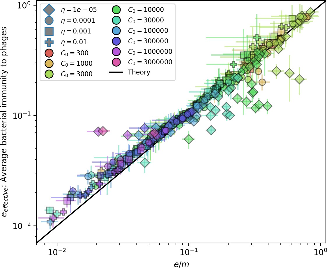
Effective vs across all simulations where on average.
Error bars are the standard deviation across three or more independent simulations. The solid black line is .
Figure 24
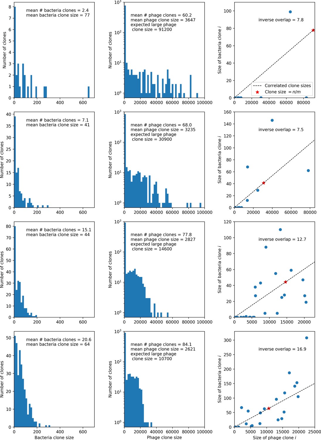
Four simulations with , , and .
From top to bottom, increases by a factor of 10 in each row, from in the top row to in the bottom row. The first two columns show clone size distributions combined from 15 time points between 2000 and 10,000 bacterial generations. Bacteria are in the left column and phages in the middle column. The third column shows the pairwise clone sizes of matching clones at the last sampled time point (9467 generations). The expected large phage clone size is the total phage population divided by the mean number of bacterial clones. The inverse overlap is , which we assume is as shown in Figure 23. The dashed line in the third column indicates the line that clone size pairs would fall on if they were perfectly correlated, and the red star indicates the mean large clone size for phages and the mean clone size for bacteria.
Figure 25
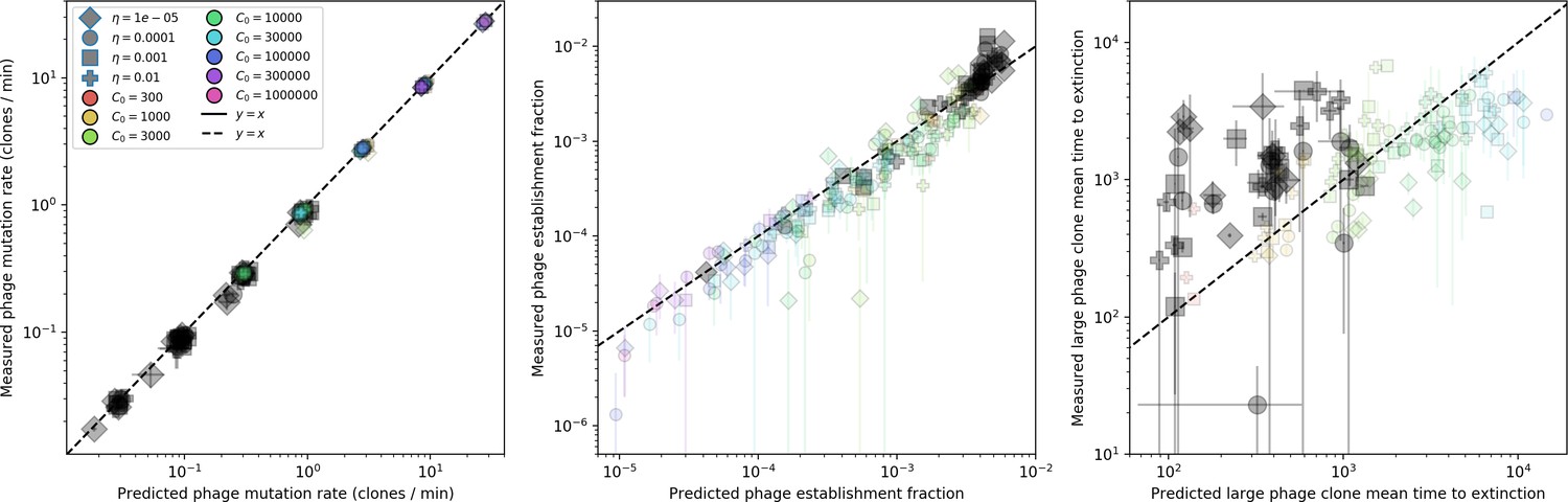
Measured simulation phage clone mutation rate, establishment fraction, and mean time to extinction as a function of the theoretical prediction for each.
Highlighted in grey are parameter combinations for which no theoretically predicted could be determined; the predicted quantity is instead calculated with the simulation mean . Error bar are the stnadard deviation across three or more independent simulations.
Figure 26
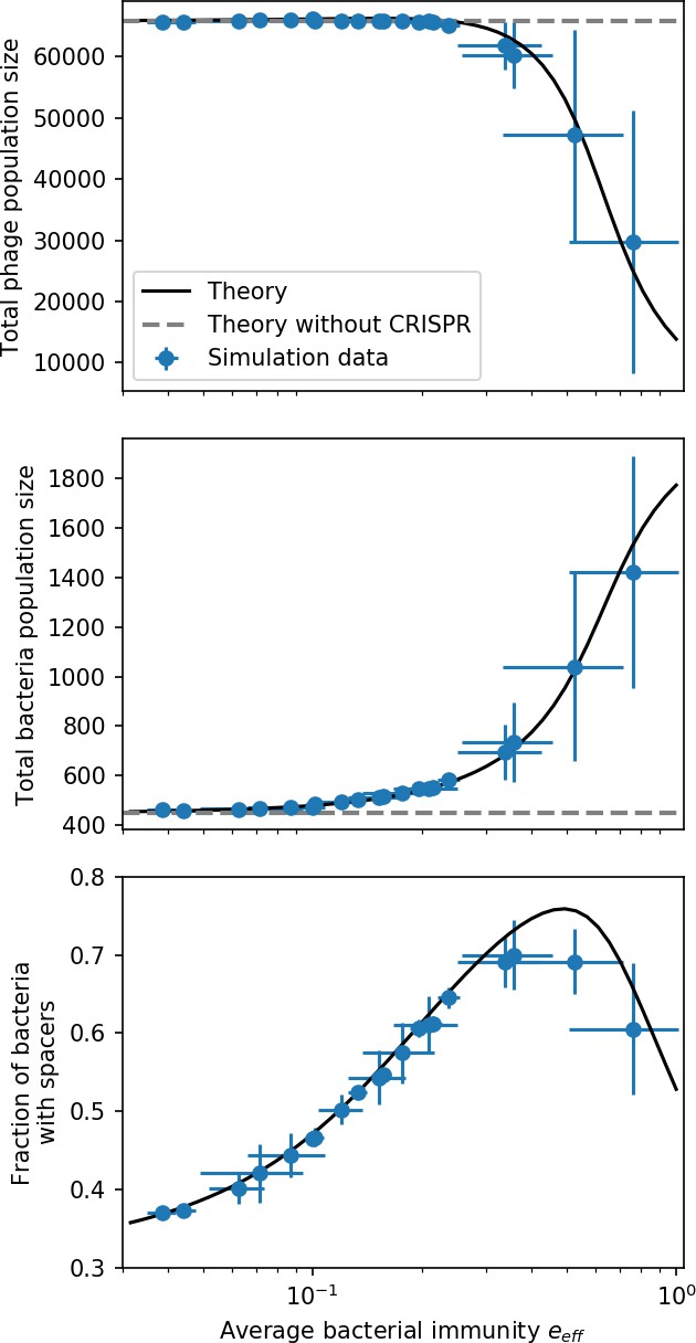
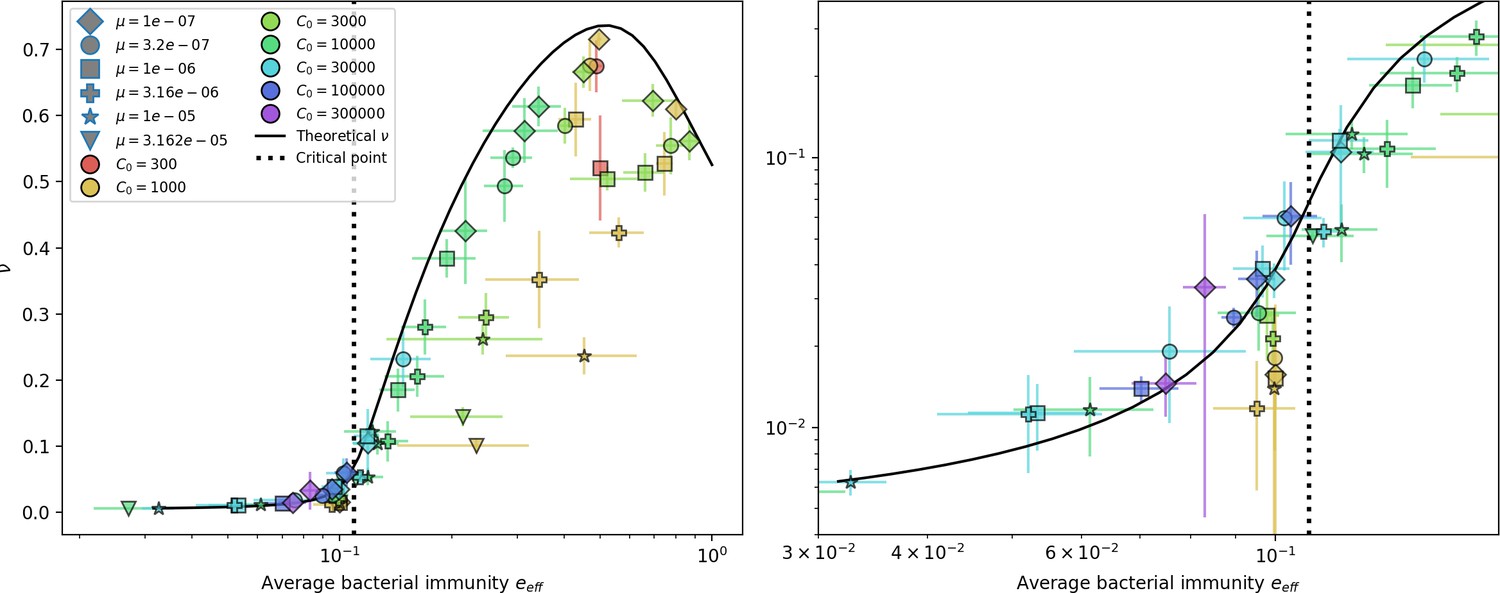
Total phage, total bacteria, and fraction of bacteria with spacers as a function of average immunity (effective ).
Blue points are simulation results. Error bars are standard deviation across three or more independent simulations. The solid black line is the solution given by Equations 42–44 (from Bonsma-Fisher et al., 2018) with the parameter replaced by effective . The horizontal grey dashed line corresponds to the no-CRISPR () mean-field solution (derived in Bonsma-Fisher et al., 2018).
Figure 27
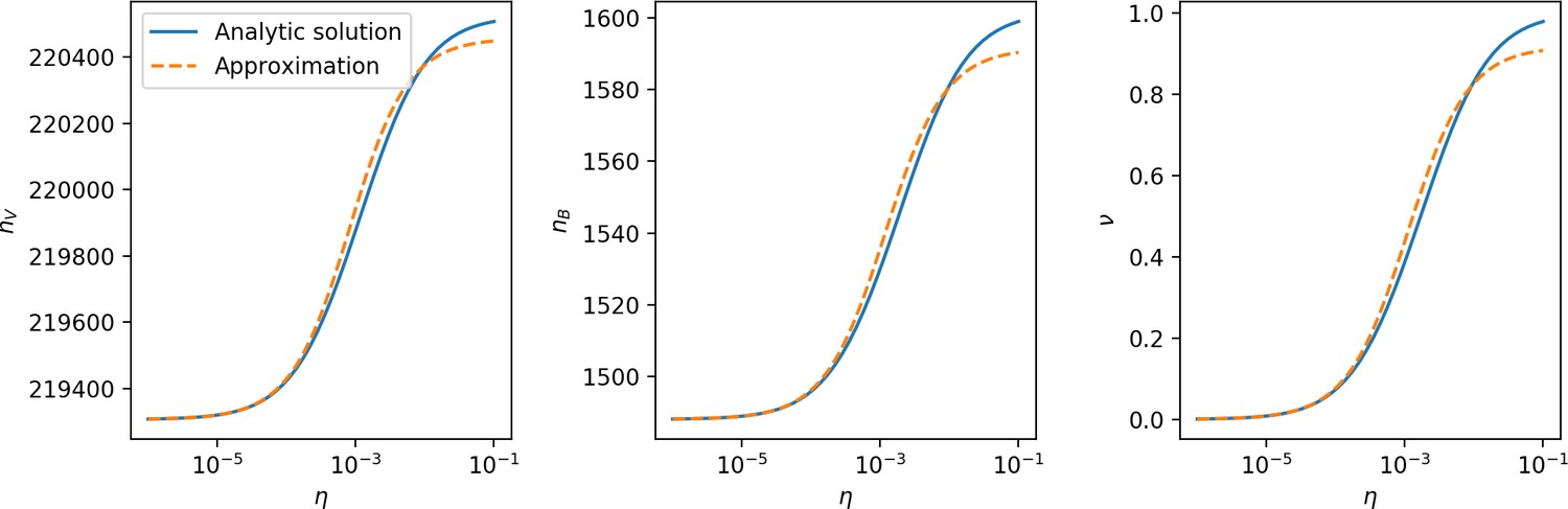
, , and vs. for , approximating .
Figure 28
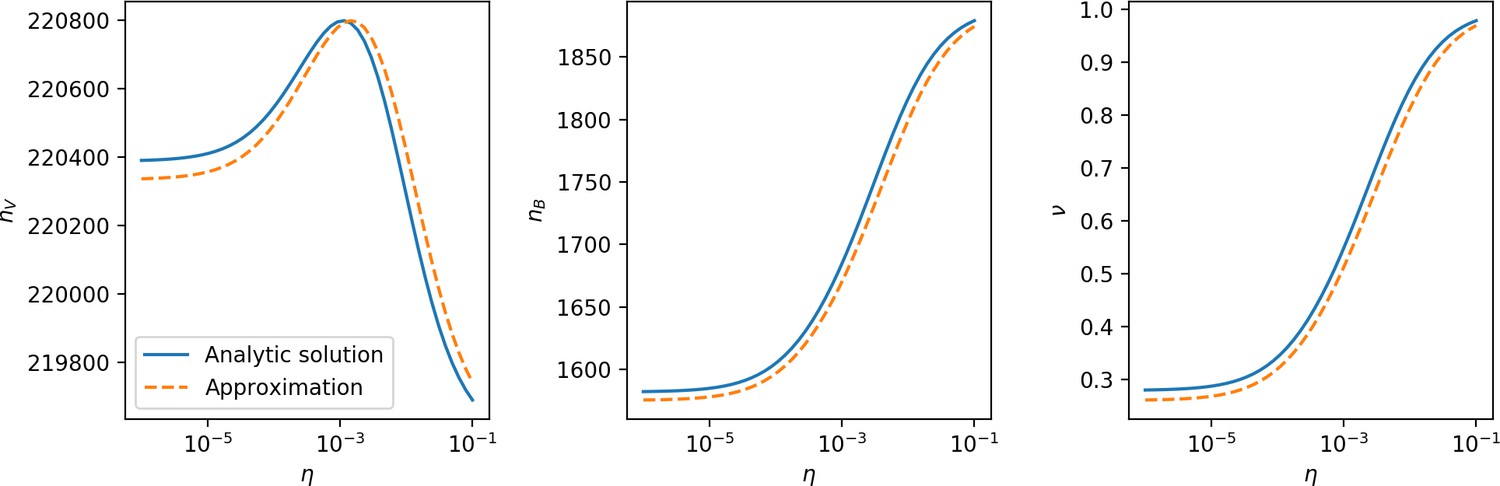
, , and vs for , approximating .
Figure 29
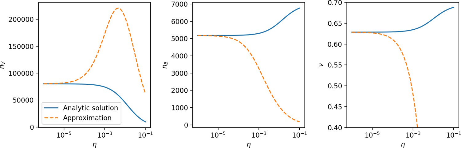
, , and vs. for , approximating .
Figure 30
Fraction of bacteria with spacers vs. effective .
The solid line is the full numerical theoretical solution. The dashed black line is given by Equation 58. Error bars are the standard deviation across three or more independent simulations.
Figure 31
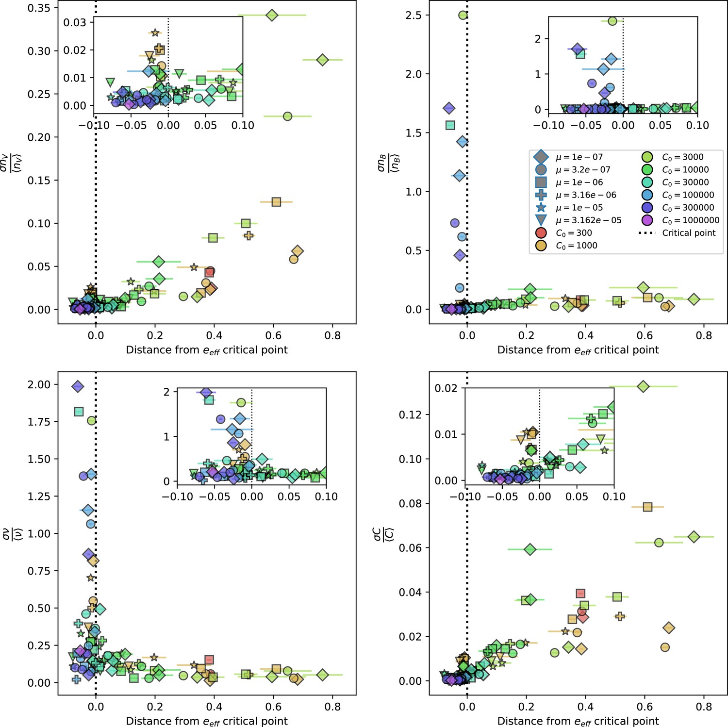
Population standard deviation divided by population mean as a function of the distance from the average immunity critical point given by Equation 58.
Insets show a smaller x-axis range for the same quantities. Total phage (top left), total bacteria (top right), fraction of bacteria with spacers (bottom left) and total nutrients (bottom right) are plotted. X error bars are the standard deviation across three or more independent simulations.
Figure 32

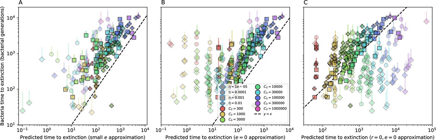
Approximate phage time to extinction vs. numerically calculated theoretical time to extinction, where the approximate time to extinction is given by (Koskella, 2014).
The full theoretical predicted value of is used in the approximate expression.
Figure 33
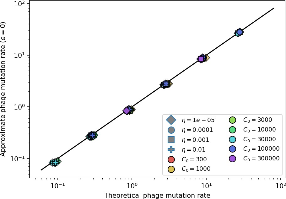
Approximate phage mutation rate for vs theoretical phage mutation rate.
Figure 34
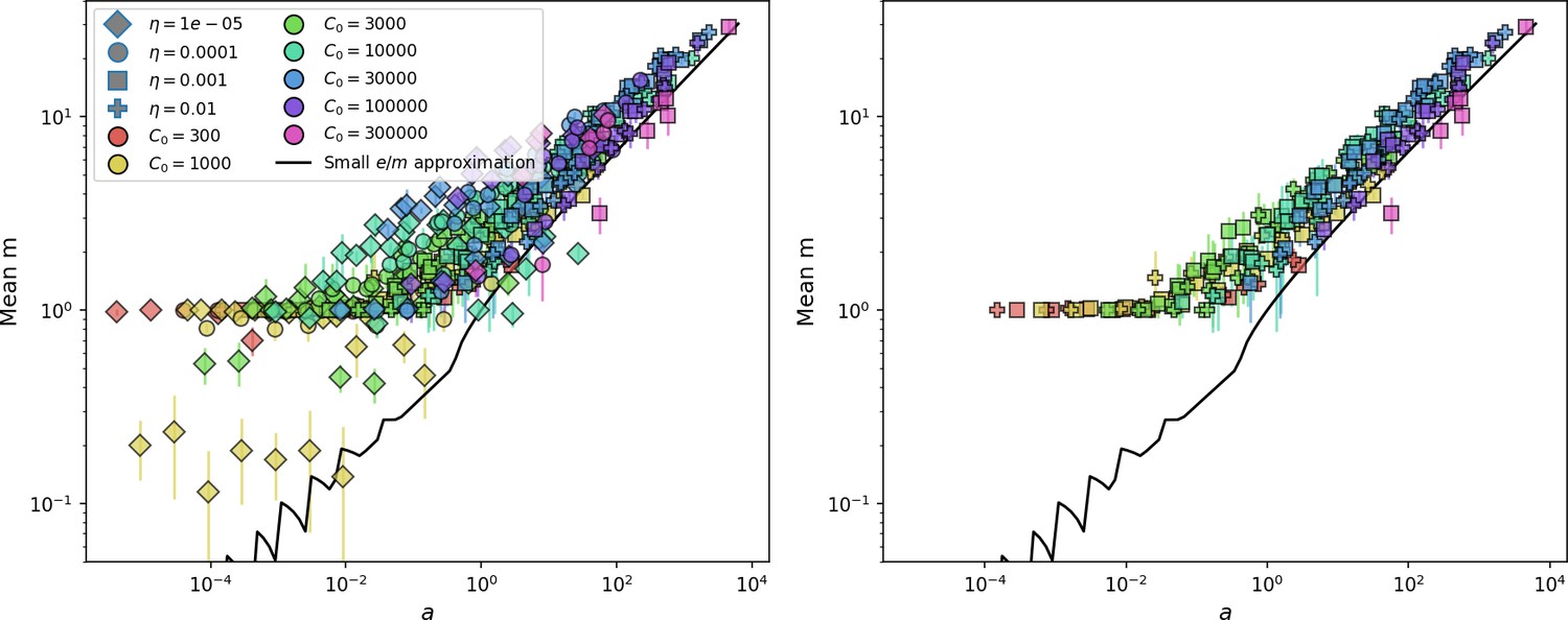
Measured mean in simulations vs. as given by Equation 81.
The solid line is vs. solved numerically using Equation 113. The right panel shows the same but with the two lowest values of removed. Error bars are the standard deviation across three or more independent simulations.
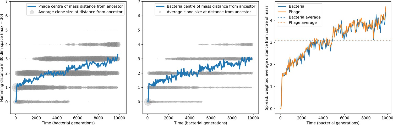
Figure 35
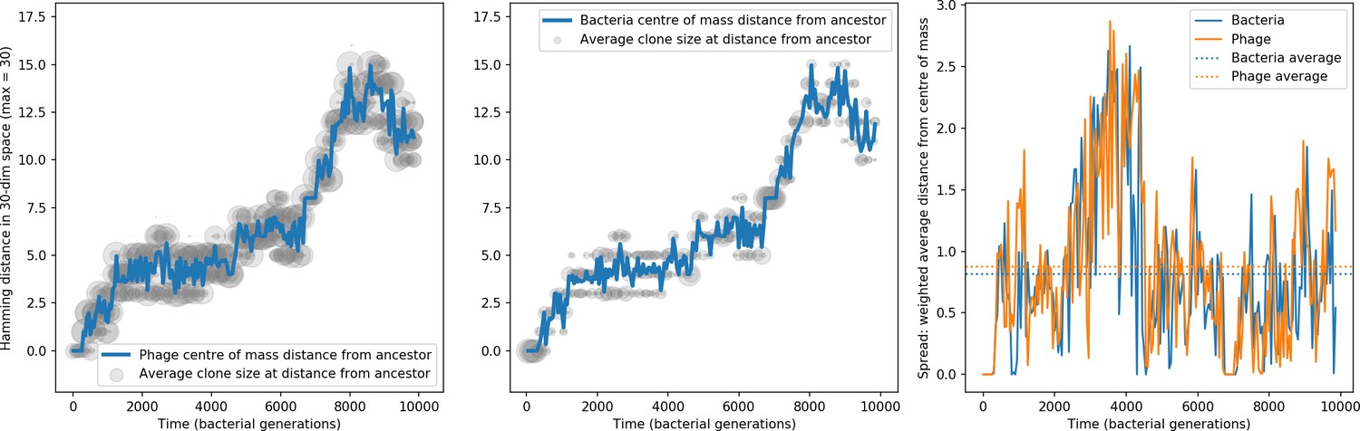
Phage and bacteria centre of mass distance from the original phage and bacteria sequences.
The centre of mass distance is plotted in blue for phage (left) and bacteria (centre). Grey circles represent the size of clonal subpopulations at each distance from the ancestor sequence (arbitrary scale). The third panel shows the weighted average distance of the population from the centre of mass at that timepoint, a measure of the spread in sequences present at any time. In this simulation , , , , and mean .
Figure 36
Phage and bacteria centre of mass distance from the original phage and bacteria sequences.
The centre of mass distance is plotted in blue for phage (left) and bacteria (centre). Grey circles represent the size of clonal subpopulations at each distance from the ancestor sequence (arbitrary scale). The third panel shows the weighted average distance of the population from the centre of mass at that timepoint, a measure of the spread in sequences present at any time. In this simulation , , , , and mean .
Figure 37
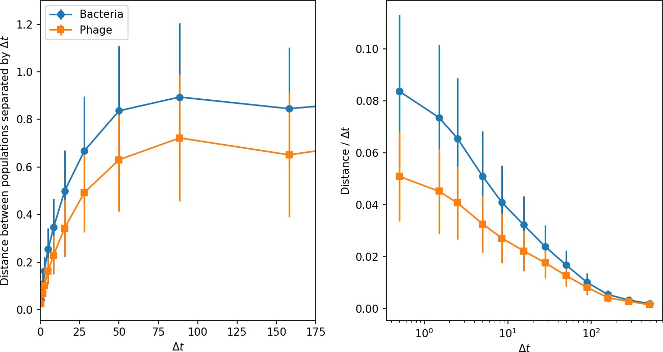
Phage and bacteria centre of mass distance from the centre of mass at time (left) and the distance divided by the time interval (right).
Distances are averaged over the entire simulation at steady state; error bars are standard deviation. Simulation parameters are , , , , and mean .
Figure 38

Maximum distance from ancestor population for bacteria vs. phage.
The maximum distance is highly correlated, indicating that the bacteria population tracks the phage population closely. Error bars are the standard deviation across three or more independent simulations.
Figure 39
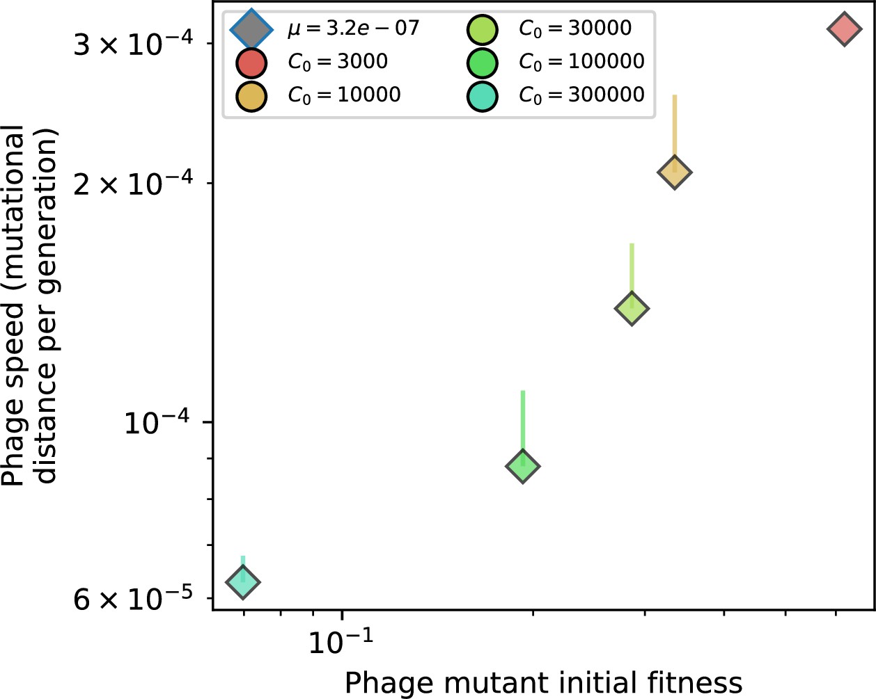
Phage mutational distance per generation vs. initial phage mutant fitness for simulations with , , and .
Error bars are the standard deviation across multiple independent simulations and are shown in the positive direction only.
Figure 40

Average population distance from the centre of mass at steady state for bacteria (left) and phages (right) vs. mean for simulations with one original phage clone ancestor.
The dashed line is , a purely phenomenological choice. Error bars are the standard deviation across three or more independent simulations.
Figure 41
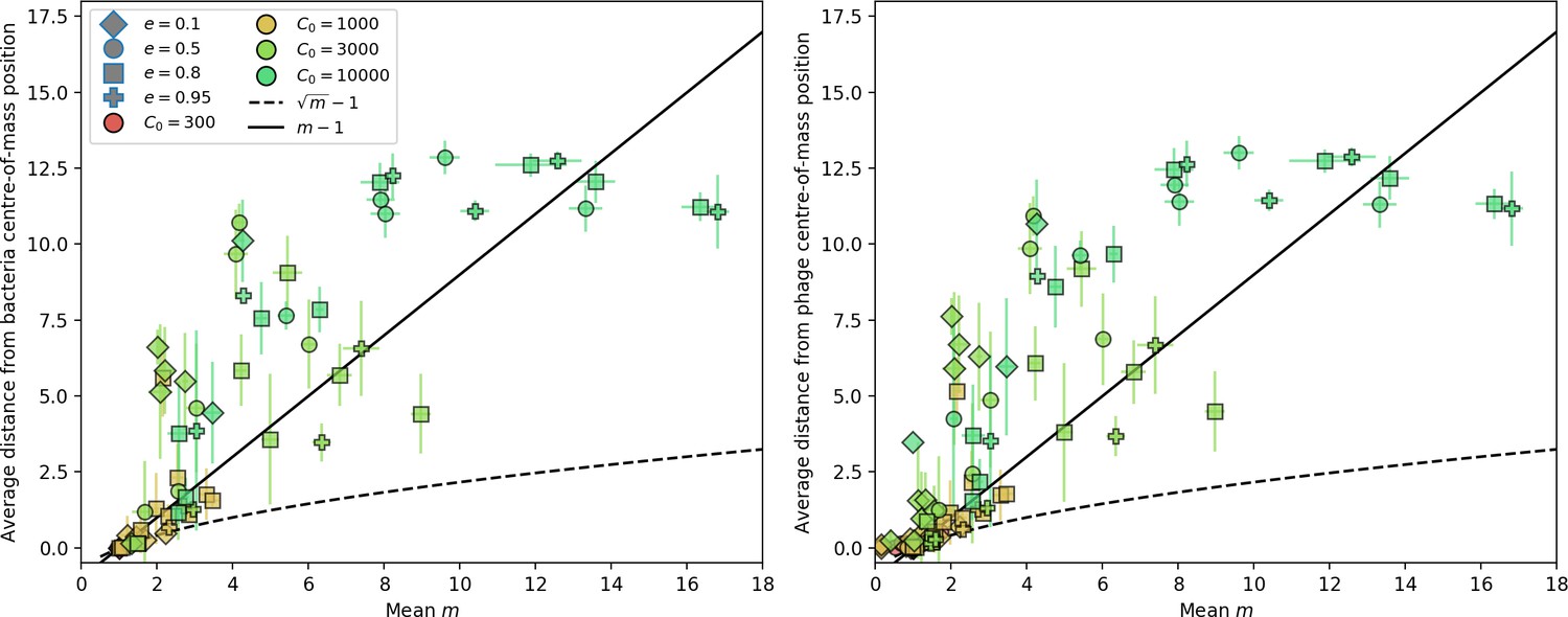
Average population distance from the centre of mass for bacteria (left) and phages (right) vs. mean for simulations with 50 original phage clones.
The dashed line is and the solid line is . Error bars are the standard deviation across three or more independent simulations.
Figure 42

A frame from a simulation movie at 5000 generations with , , , , initial .
Phages are on the left, bacteria with spacers on the right.
Figure 43
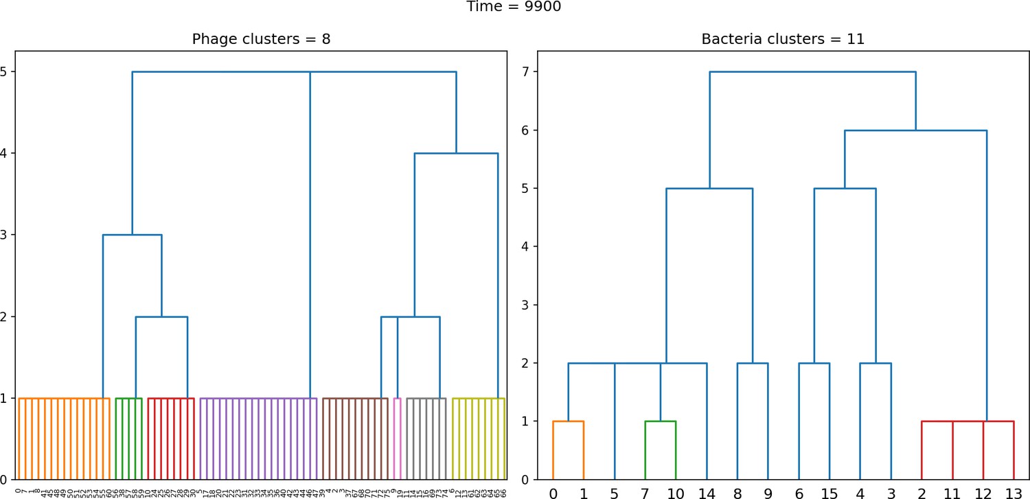
Dendrogram resulting from agglomerative clustering with the L1 norm and linking clusters using the minimum distance between members.
The number of clusters is determined with a cutoff at a distance of 2. , , , , initial .
Figure 44
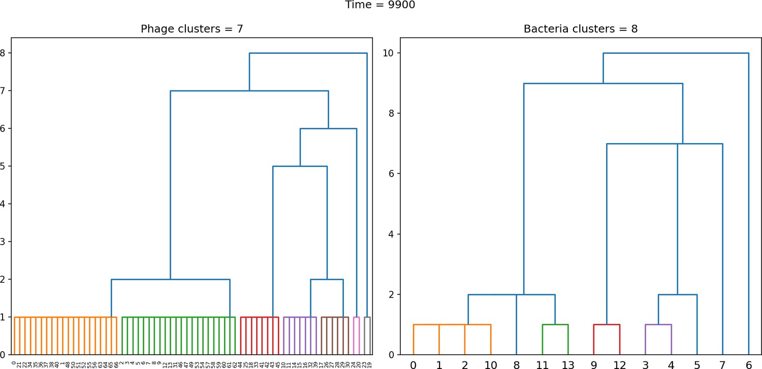
Dendrogram resulting from agglomerative clustering with the L1 norm and linking clusters using the minimum distance between members.
The number of clusters is determined with a cutoff at a distance of 2. , , , , initial .
Figure 45
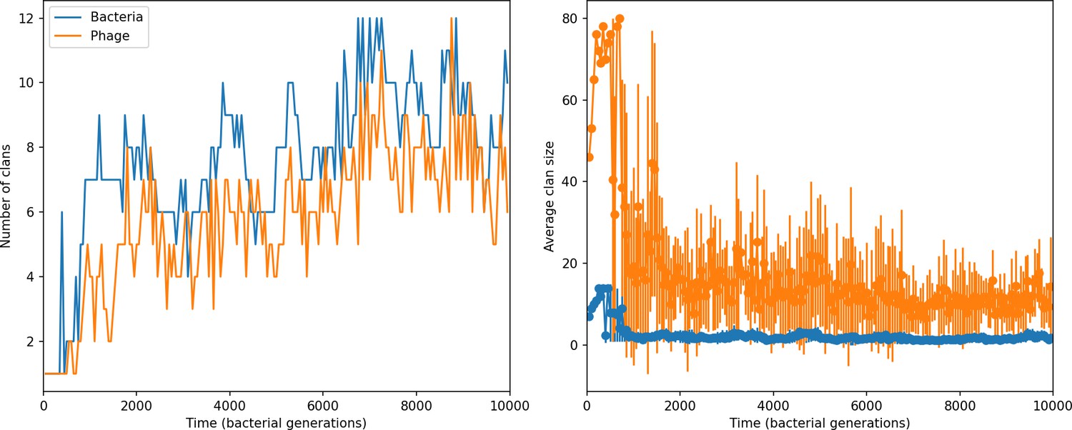
Clan number and size over time in a simulation with , , , , initial .
Figure 46
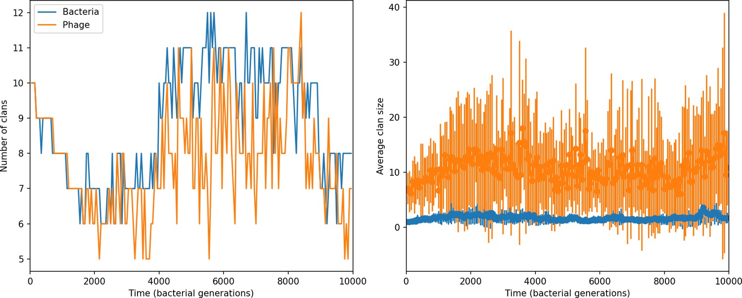
Clan number and size over time in a simulation with , , , , initial .
Figure 47
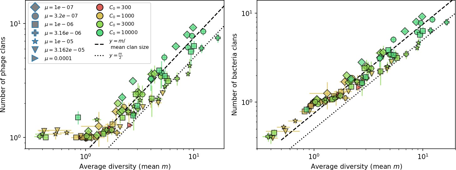
Average clan number vs. for all simulations that begin with 10 clones.
The dashed lines are divided by the mean bacterial clan size () and . Error bars are the standard deviation across three or more independent simulations.
Figure 48
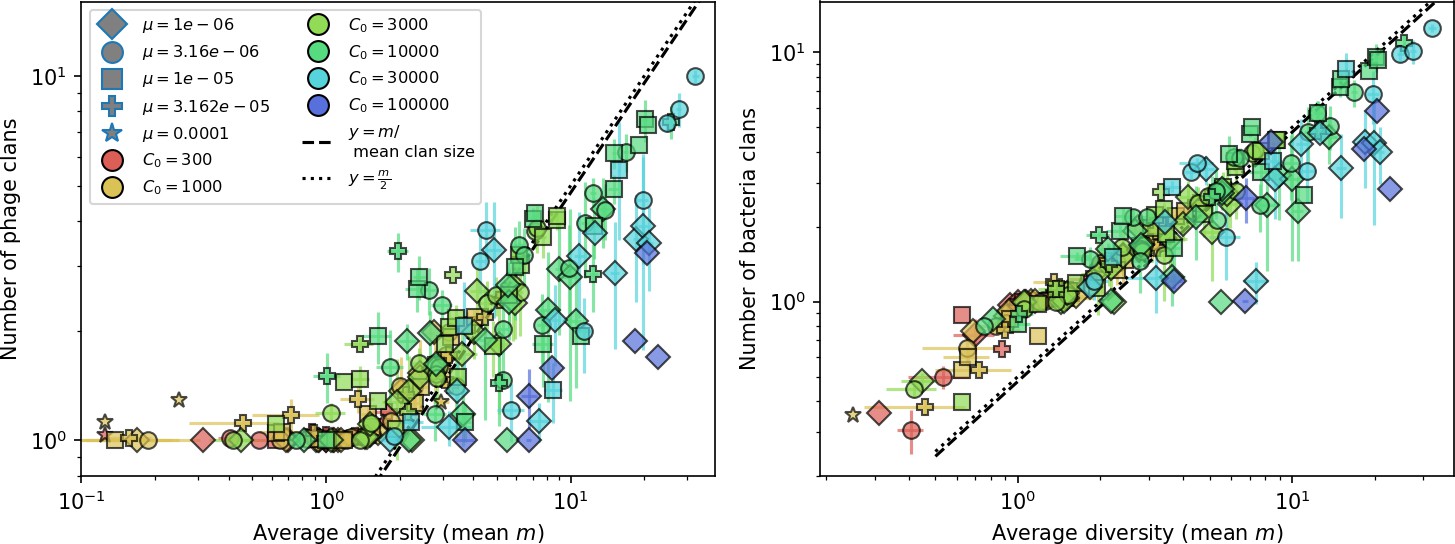
Average clan number vs. for all simulations that begin with one clone with .
The dashed lines are divided by the mean bacterial clan size and . Error bars are the standard deviation across three or more independent simulations.
Figure 49
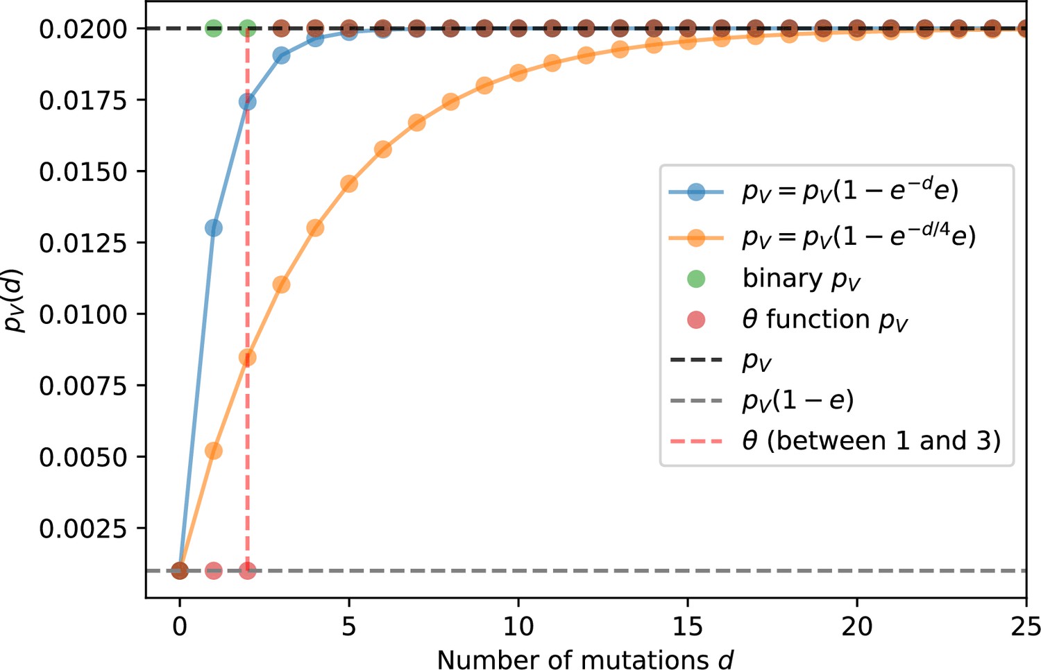
Phage infection success probability as a function of mutational distance between spacers and protospacers for different definitions and degrees of cross-reactivity.
Definitions are plotted for , .
Figure 50
Average immunity vs. diversity with different degrees of cross-reactivity for simulations with , .
Dashed lines are simulations with cross-reactivity, solid line is simulations without cross-reactivity. Error bars are the standard deviation across three or more independent simulations.
Figure 51

Mean phage clone size (top) and mean bacteria clone size (bottom) relative to time of phage mutation for different definitions of .
These simulations begin with one initial phage clone and parameters , , , .
Figure 52
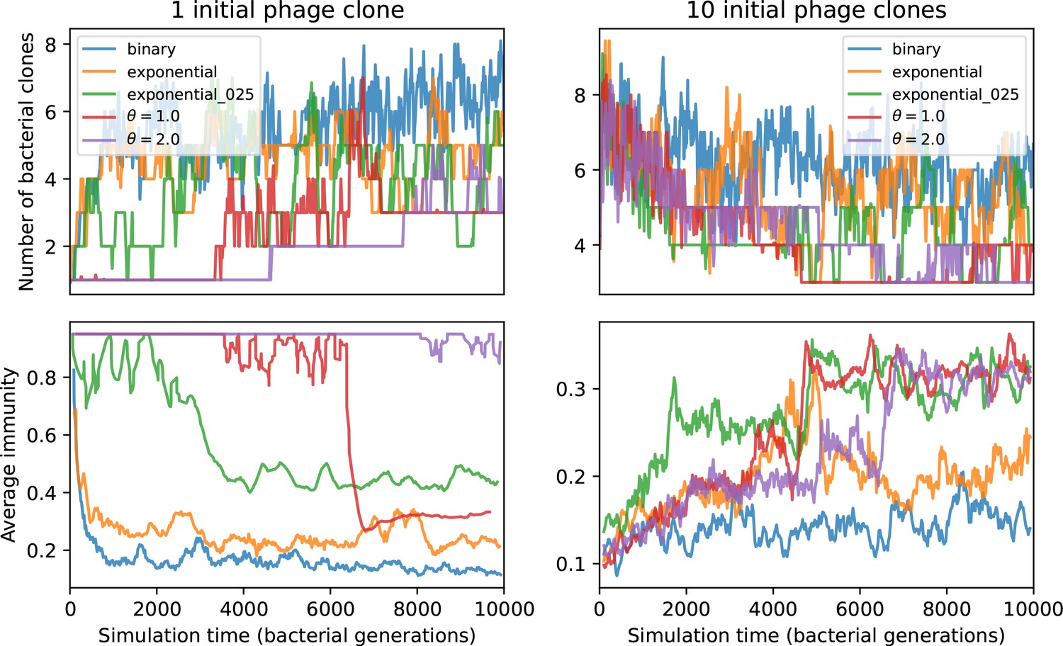
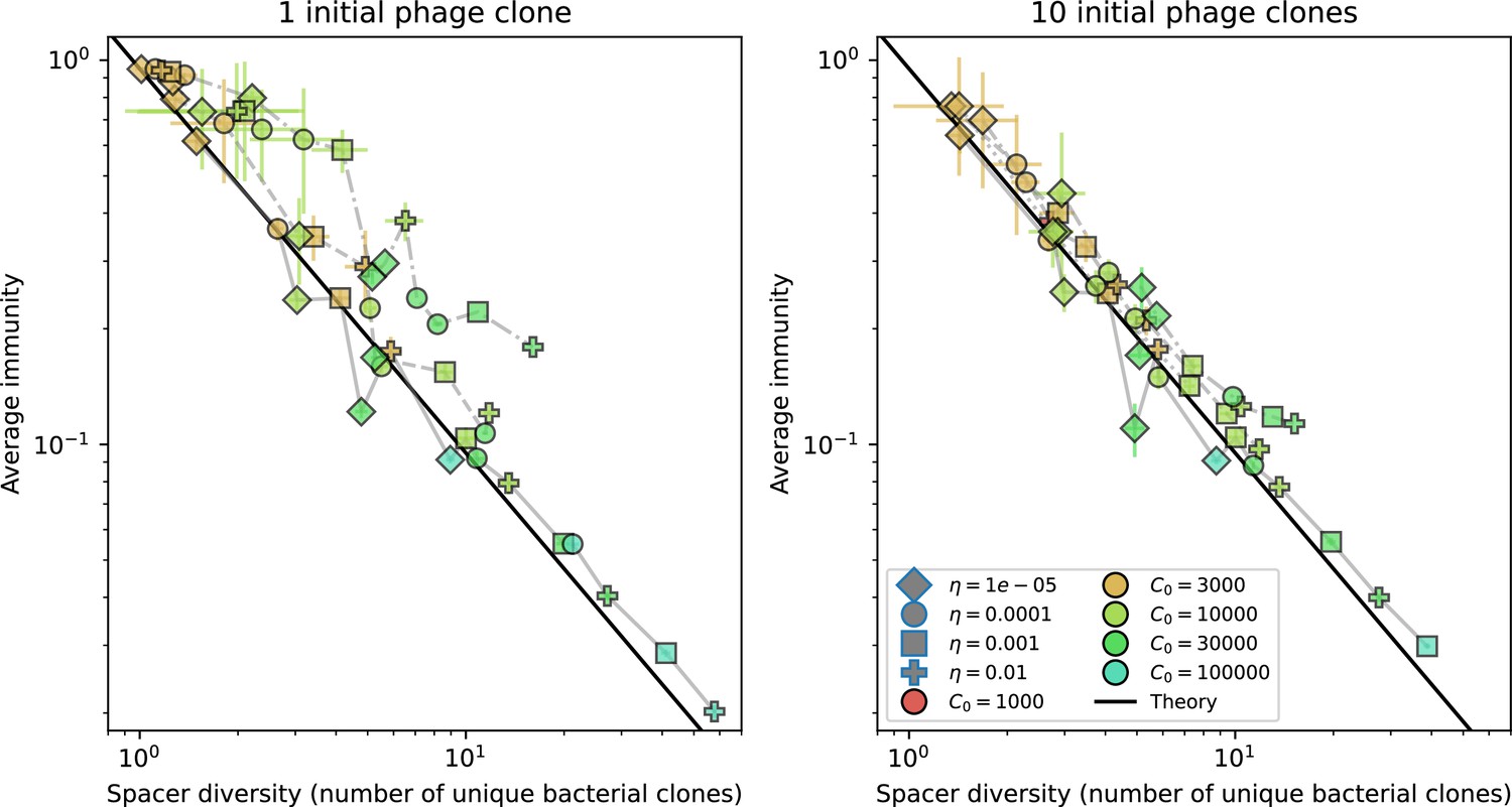
Number of bacterial clones (top) and average immunity (bottom) for simulations beginning with either 1 phage clone (left) or 10 phage clones (right).
These simulations have parameters , , , .
Figure 53
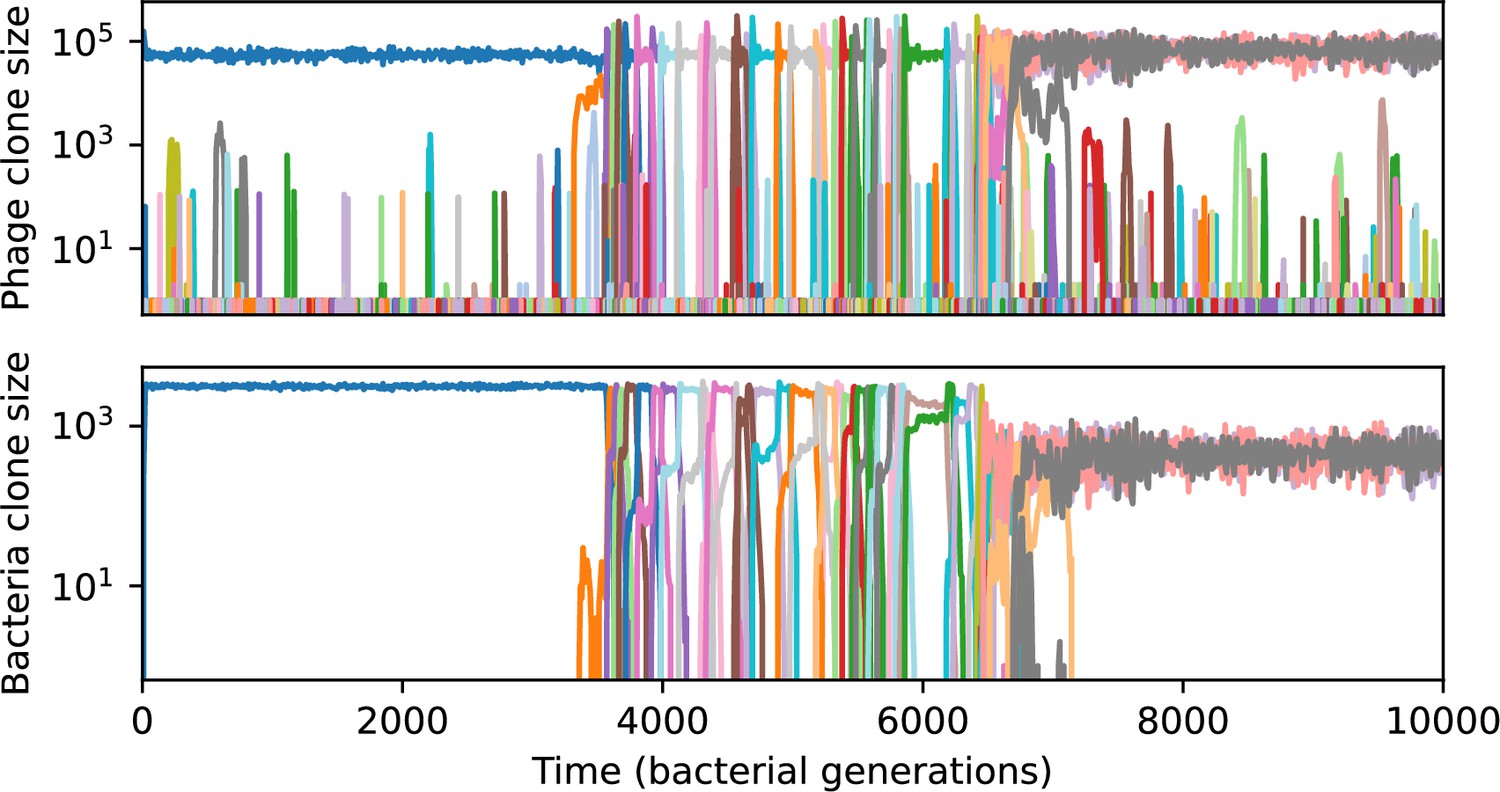
Phage clone size (top) and bacteria clone size (bottom) in a simulation with cross-reactivity (step function CRISPR effectiveness with ).
Figure 54
Phage clone size (top) and bacteria clone size (bottom) in a simulation with cross-reactivity (step function CRISPR effectiveness with ).
This simulation has one initial phage clone and parameters , , , and . Later times in this simulation are shown in Figure 55.
Figure 55
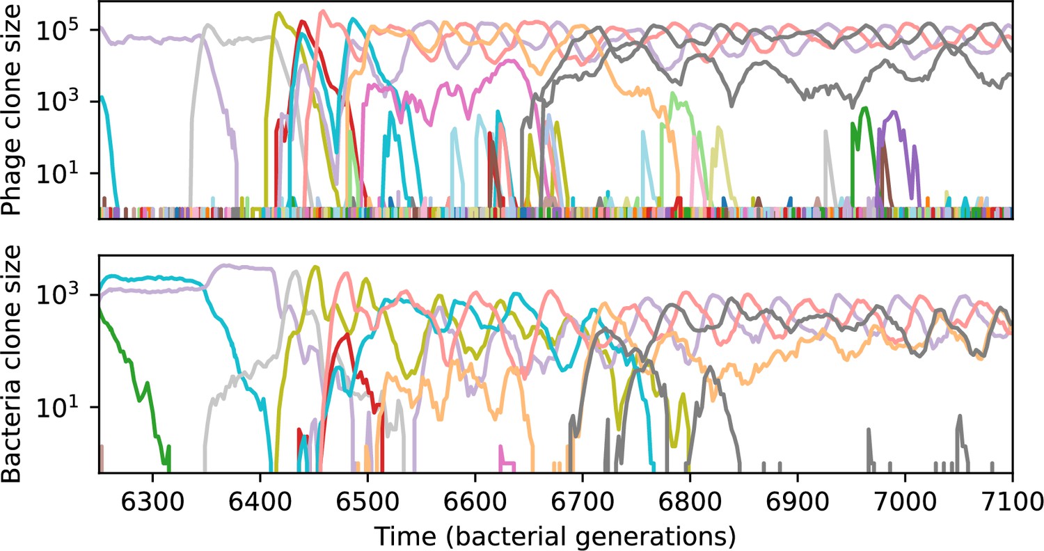
Phage clone size (top) and bacteria clone size (bottom) in a simulation with cross-reactivity (step function CRISPR effectiveness with ) showing the switch between a travelling wave and low turnover regime.
This simulation has one initial phage clone and parameters , , , and . Earlier times in this simulation are shown in Figure 54.
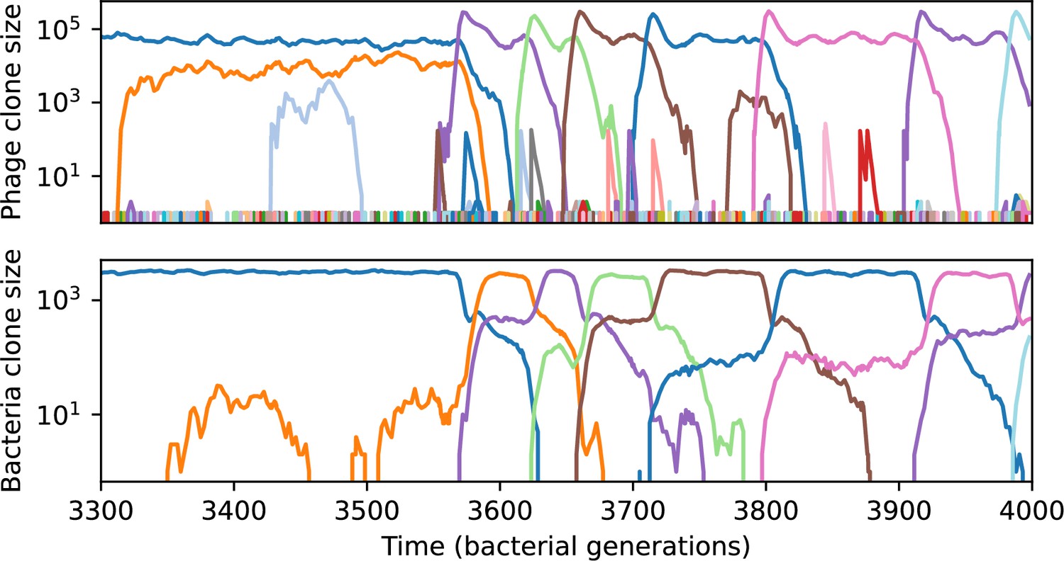
Figure 56
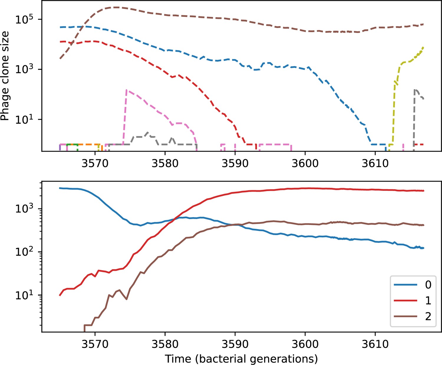
Phage clone size (top) and bacteria clone size (bottom) for a short time window of the simulation shown in Figure 54.
Large phage and bacteria clones are numbered in the legend; these numbers correspond to the numbers in Figure 57.
Figure 57

Phage infection success probability matrix for each clone shown in Figure 56.
Dark blue is low infection success, light blue is high infection success.
Figure 58

Mean phage clone size (top) and mean bacteria clone size (bottom) relative to the time of phage clone mutation, either normalized to surviving clones (left) or averaged over all trajectories (right) for the simulation shown in Figure 54 (, , ).
Clones in the travelling wave regime (4000–6200 generations, orange) grow much more quickly than clones in the initial low-turnover regime (1000–3200 generations, blue) or the final low turnover regime (7000–10,000 generations, green). The black dashed line is the mean clone size for a simulation with the same parameters but without cross-reactivity.
Figure 59
A slow-switching cross-reactivity regime for the simulation shown in Figure 54.
(Left) A subset of clone trajectories for phages (top) and bacteria (bottom) in a simulation with cross-reactivity (step function CRISPR effectiveness with ). Three trajectories are highlighted and coloured to show increasing time. The population is in a regime where matching clones are offset: because clones that are one mutation apart have the same complete immune overlap, the highlighted clones have large bacterial clone size well after the matching phage clone goes extinct. (Right) The clone size of the highlighted trajectories shown as a function of the bacterial marginal immunity against a particular phage clone (top) or the marginal immunity of a particular bacteria clone (bottom).
Figure 60

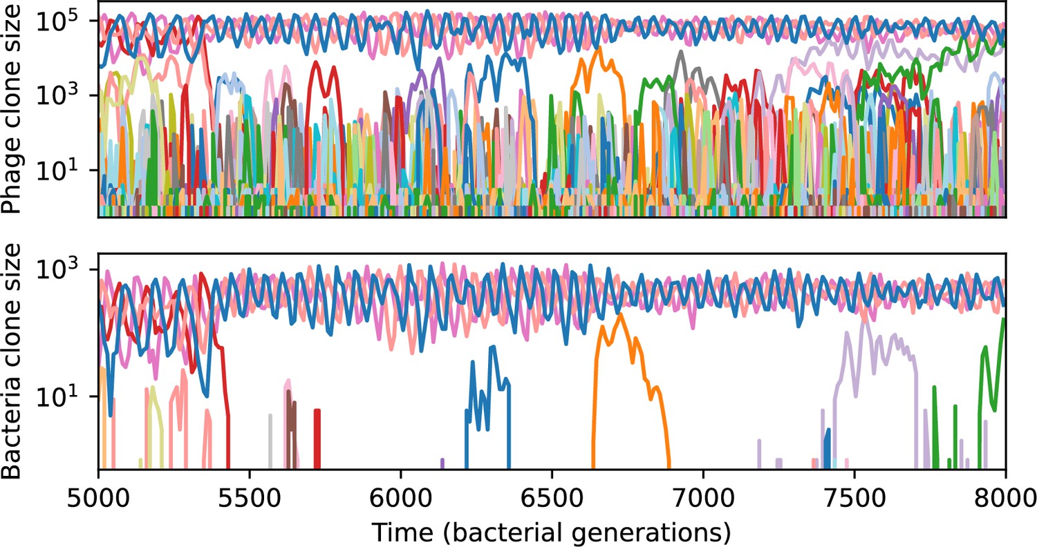
Cross-reactivity leads to persistent oscillations.
(A) A subset of clone trajectories for phages (top) and bacteria (bottom) in a simulation with no cross-reactivity. Transient oscillations occur. One trajectory is highlighted and coloured to show increasing time. (B) The highlighted trajectory in (A) is shown as a function of the marginal immunity for phages (top) and bacteria (bottom). Clones experience an oscillating fitness that depends on their overlap from the other population. Arrows indicate the direction of increasing time in the oscillation. (C) A subset of clone trajectories for phages (top) and bacteria (bottom) in a simulation with cross-reactivity (step function CRISPR effectiveness with ). The population is in a regime where several clones experience persistent and rapid oscillations. One trajectory is highlighted and coloured to show increasing time. (D) The highlighted trajectory in (C) is shown as a function of the marginal immunity for phages (top) and bacteria (bottom). Clones experience an oscillating fitness that depends on their overlap from the other population. Arrows indicate the direction of increasing time in the oscillation. For all simulations , and .
Figure 61
Phage clone phylogenies for four simulations with different cross-reactivities and a higher mutation rate than shown in main text Figure 4: no cross-reactivity (A) and step-function cross-reactivity with (B, ) (C), and (D).
All simulations share all other parameters: . Phage clones are plotted at the first time they pass a population size of 2 (to remove clutter from many new mutations destined for extinction), and the size of each circle is logarithmically proportional to the maximum size reached by that clone. Colours indicate the time of extinction of each clone. For each simulation with cross-reactivity, the left inset shows phage (top) and bacteria (bottom) clone sizes over time; colours indicate unique clone identities.
Figure 62
Phage clone size (top) and bacteria clone size (bottom) for a short time window of the simulation shown in Figure 61C.
Each of the large trajectories oscillating out of phase between 5000 and 7000 generations is at least three mutations away from all of the others; they are all outside each other’s cross-reactivity radius.
Figure 63

Matrix of mutational distance between each of the four largest phage clones shown in Figure 62; colours of those trajectories are labelled on the y axis.
Each clone is at least three mutations away from all other large clones.
Figure 64
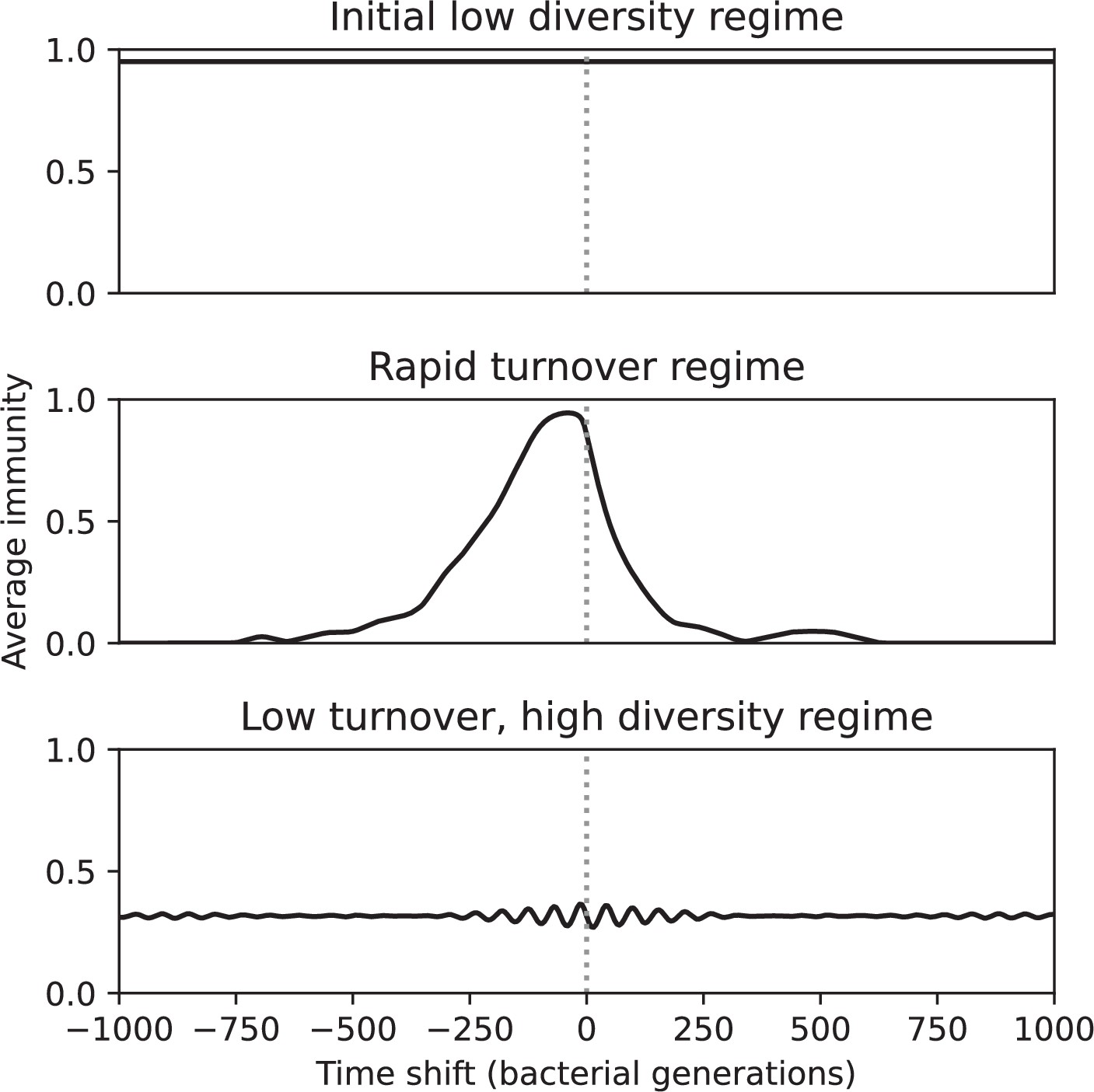
Time-shifted average immunity for three regimes of the simulation shown in Figure 54 (, , , and , step-function cross-reactivity with ).
The initial low-diversity regime (1000–3200 generations) and the low turnover, high diversity regime (7000–10,000 generations) had extremely low turnover, while the travelling wave regime (4000–6200 generations) had high average immunity near 0 delay that rapidly decayed to zero both in the past and future.
Figure 65
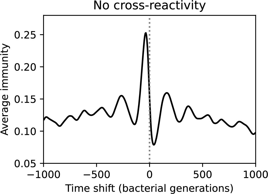
Time-shifted average immunity for the corresponding simulation to Figure 64 without cross-reactivity (, , , and ). Peak average immunity is low because of high diversity, and immunity decays very gradually to zero in both the past and future.
Figure 66
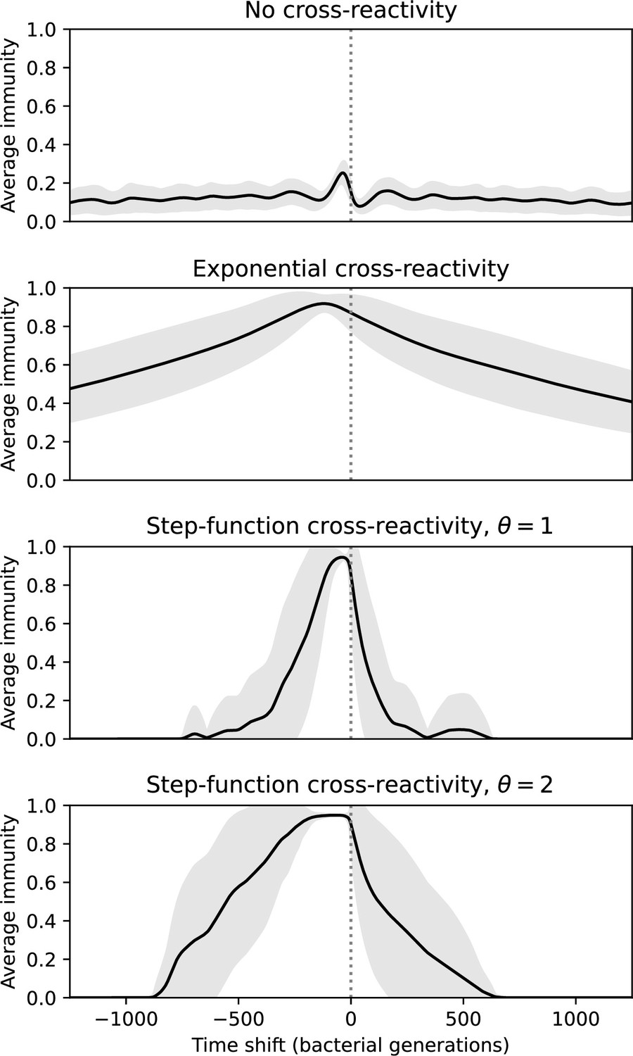
Time-shifted average immunity for four simulations with the same parameters but different types of cross-reactivity: no cross-reactivity (top), exponential cross-reactivity (middle top), step-function cross-reactivity with (middle bottom), and (bottom).
Shared parameters are , , , and . Only the travelling-wave regime of each simulation with cross-reactivity was used to compare turnover in this regime. The grey shaded region is the standard deviation across averaged data.
Figure 67
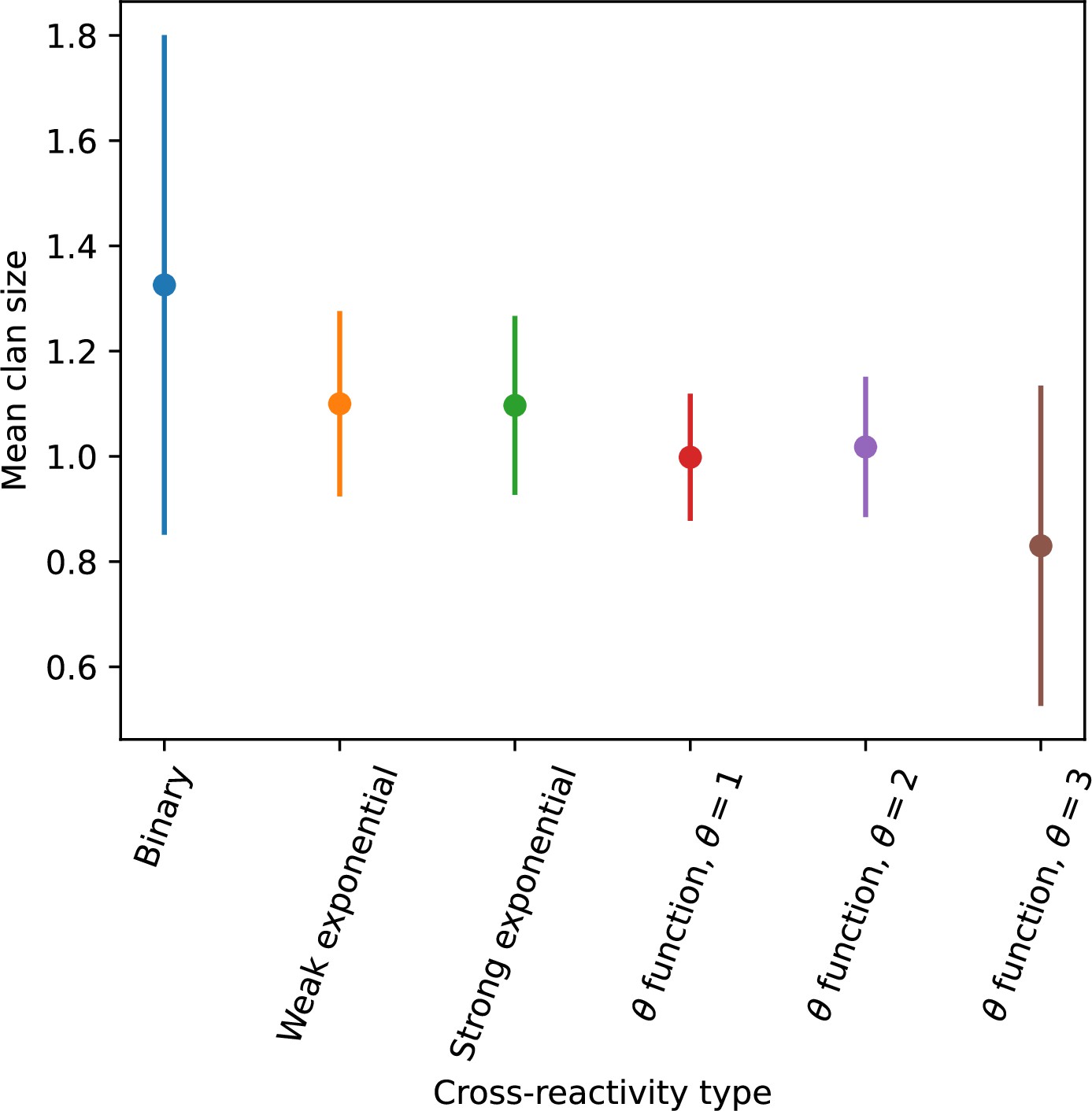
Average clan size across simulations with different parameters for different degrees of cross-reactivity with .
Error bars are the standard deviation across three or more independent simulations.
Figure 68

Average immunity vs. bacterial spacer array length for simulated distributions of protospacers and spacers.
We simulate 50 phages, each with 5 protospacers represented by letters from the alphabet, uniformly sampled. We simulate 420 bacterial spacers, drawn from the alphabet either uniformly (top row) or following an exponential distribution with mean 6 (bottom row). We construct arrays by sampling from the set of 420 spacers without replacement, either creating arrays of constant length (left column), or of variable length with a gaussian distribution (middle column) or exponential distribution (right column). Average immunity is calculated as in Equation 90 except the indices run over all arrays and not over individual sequences, and the presence of any matching pair gives perfect immunity. Blue points are average results over 50 simulations; error bars are standard deviation. The black dashed curve is given by .
Figure 69
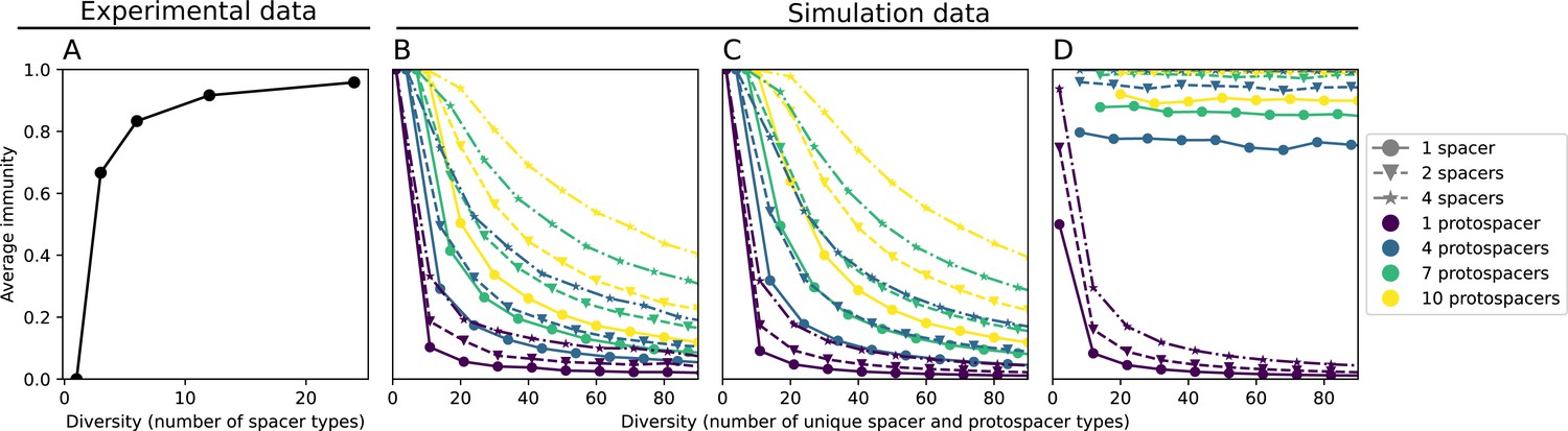
Average immunity decreases with coupled CRISPR diversity.
(A) Inferred initial average immunity as a function of diversity in the experiment of Common et al., 2020. Bacterial diversity was manipulated in the experiment by combining different numbers of bacterial clones defined by unique CRISPR spacers with a single phage strain that was able to infect only one of the clones. We calculated the expected initial average immunity based on the number of clones. (B–D) Results of a toy model of sorting a set of protospacers and spacers into arrays of variable length, either assigning protospacers fully randomly (B), as sequential mutations (C), or changing the last protospacer in the array only (D).
Figure 70

Average immunity vs. diversity (number of unique types) for simulated distributions of spacers and protospacers with different bacterial array sizes (increasing top to bottom) and different numbers of protospacers per phage (increasing left to right).
Bacterial array sizes are drawn from a Gaussian distribution with mean given by the array mean for each row and a standard deviation of 2. Points are averages across 50 independent runs.
Figure 71
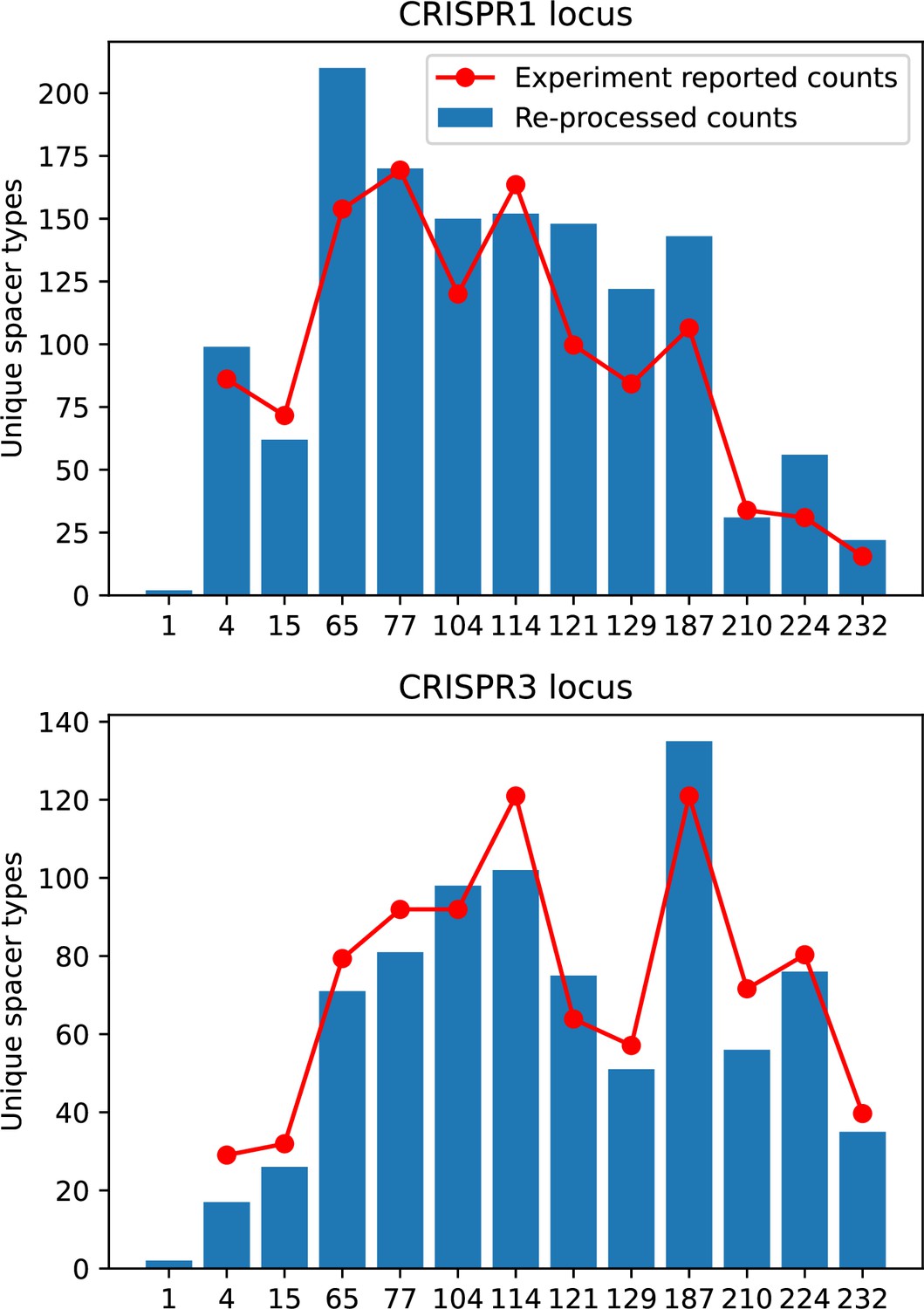
Unique spacer types detected in our analysis of data from Paez-Espino et al., 2015 after grouping by 85% average similarity and removing single spacer counts (blue bars).
Counts reported in Paez-Espino et al., 2015 are red points.
Figure 72

Total reads per time point that match phage (blue) or bacteria (orange).
Top: total reads. Middle: total reads divided by phage and bacteria genome sizes. Bottom: fraction of total reads matching bacteria or phages.
Figure 73
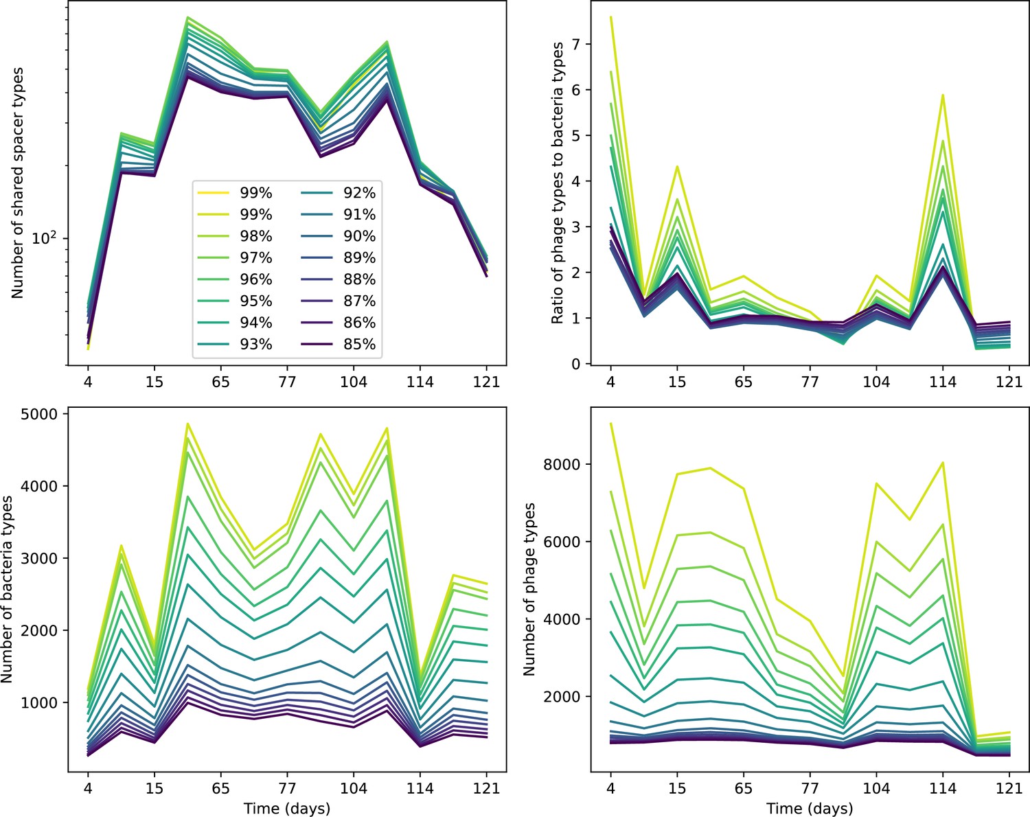
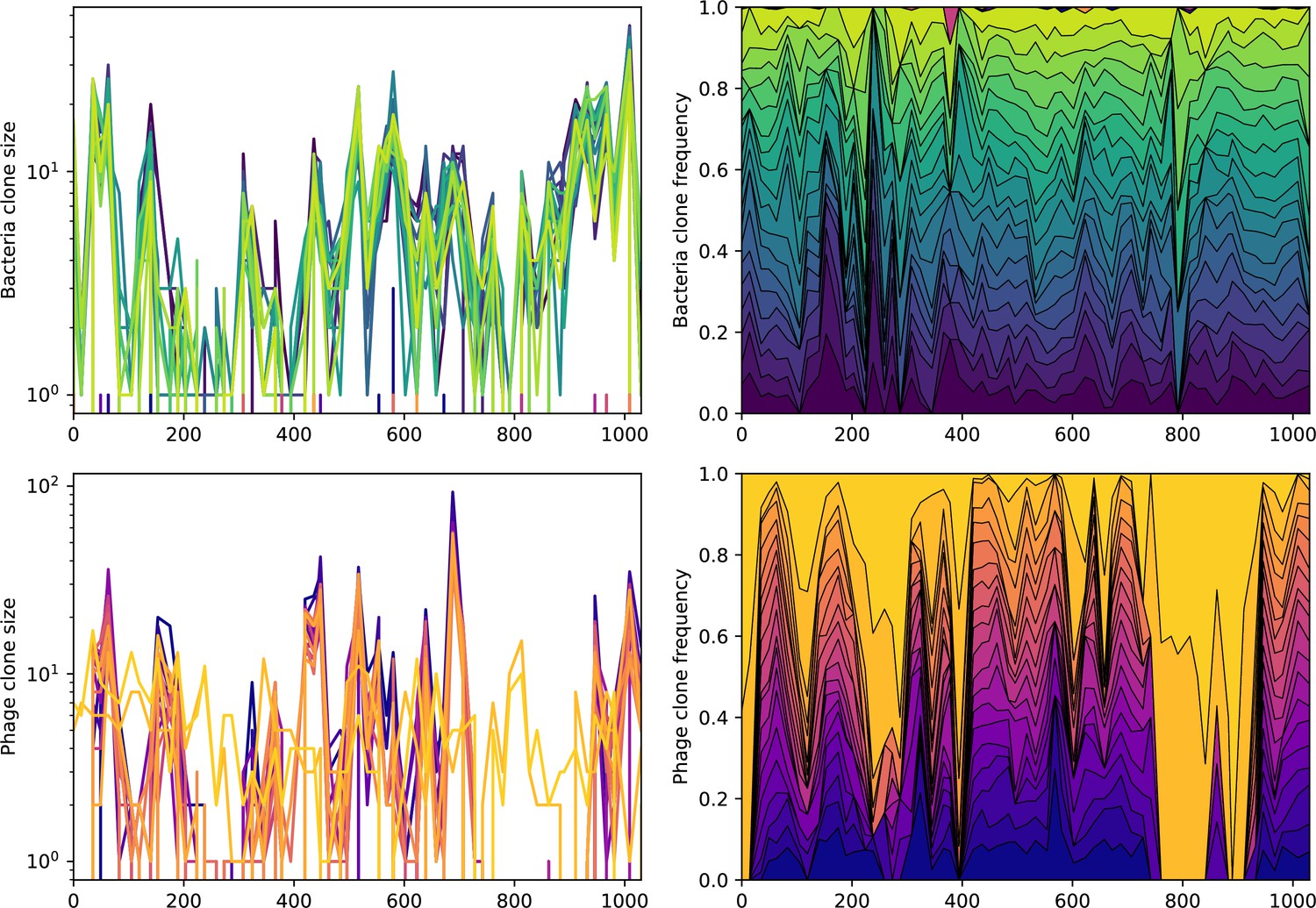
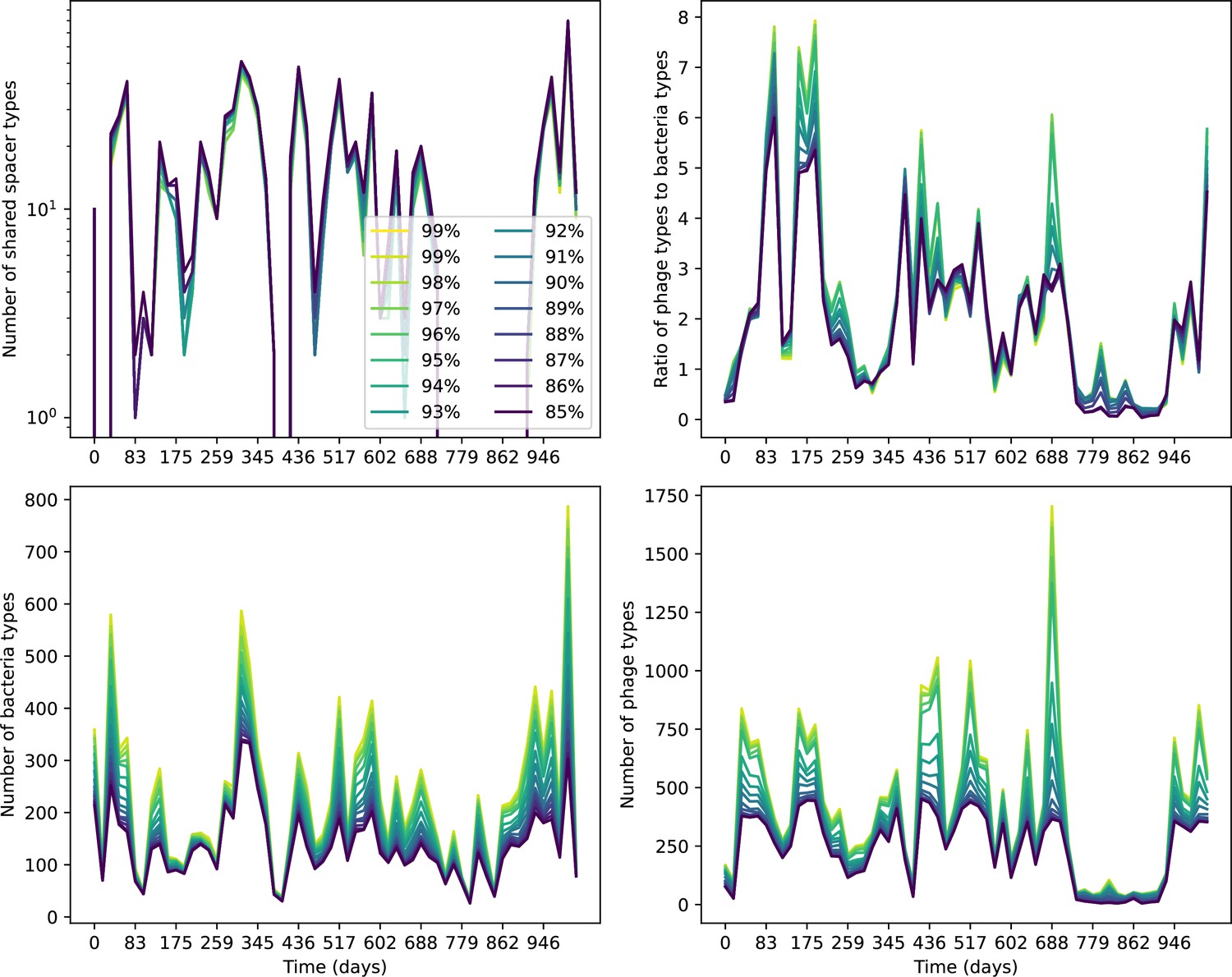
Number of shared spacer types between bacteria and phage (top left), ratio of the number of phage types to the number of bacteria types (top right), number of bacteria types (bottom left), and number of phage types (bottom right) as a function of the sampling date for data we analysed from Paez-Espino et al., 2015.
Colours indicate different similarity grouping thresholds. Spacer counts include wild-type spacers, and protospacers are included only if they possess a perfect PAM. Data is summed over CRISPR1 and CRISPR3. All sequences are included regardless of abundance.
Figure 74

Total phage and bacteria population size for the MOI2B experiment in Paez-Espino et al.Paez-Espino et al., 2015.
Circles are points digitized from Figure 1A in Paez-Espino et al., 2015; squares are the population size interpolated to match the sequencing dates in the experiment.
Figure 75
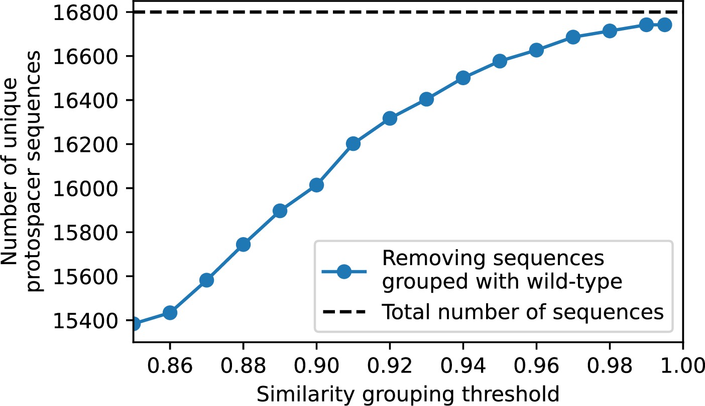
Total number of unique protospacer sequences after removing all sequences that cluster with wild-type sequences at different similarity thresholds.
Only protospacers with a perfect PAM are included.
Figure 76
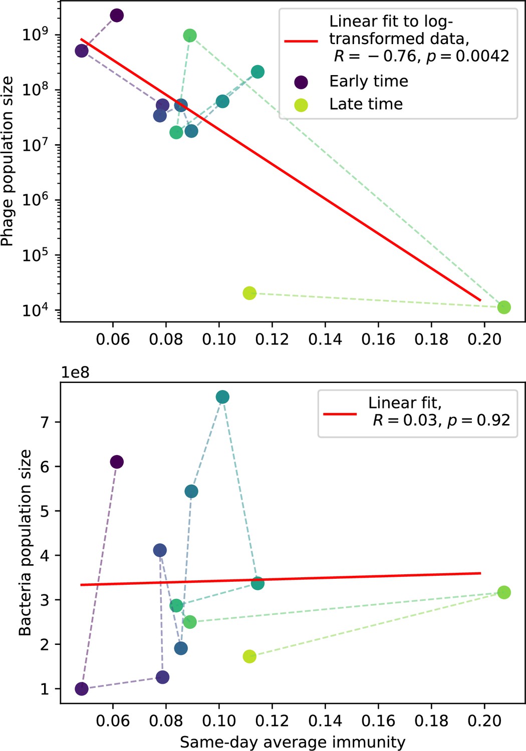
Phage (top) and bacteria (bottom) population size vs. average immunity calculated with data from Paez-Espino et al., 2015.
Protospacers are included if they have a perfect PAM, and all wild-type spacers are included. Spacers and protospacers are grouped with an 85% similarity threshold. Colours from blue to yellow indicate increasing time.
Figure 77
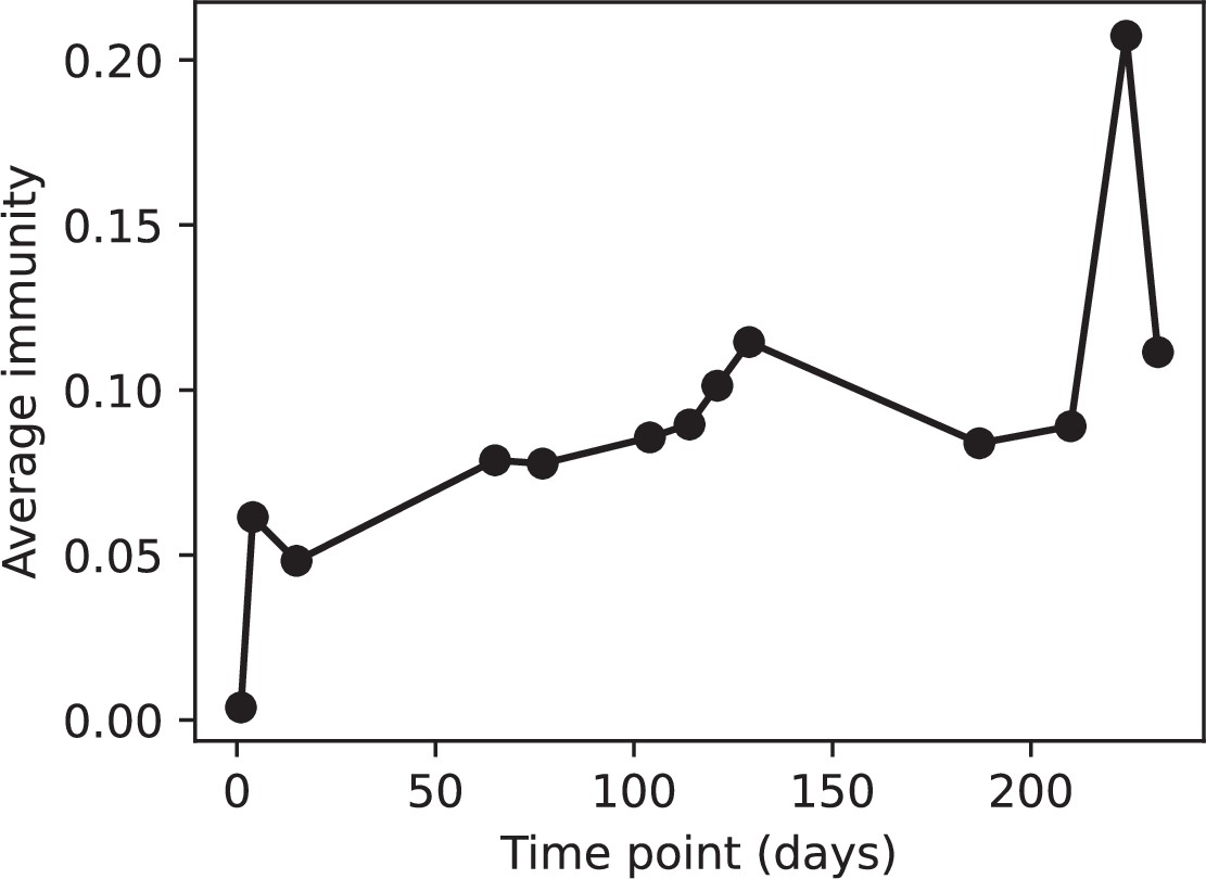
Average immunity vs time in the MOI-2B experiment.
Protospacers are included if they have a perfect PAM, and all wild-type spacers are included. Spacers and protospacers are grouped with an 85% similarity threshold.
Figure 78

Histogram of reads that matched both the Gordonia MAG and either phage reference genome vs the base-10 log difference in e-value between the matches for accession SRR9260993.
A positive value means the bacteria match has a lower e-value than the phage match. The vertical dashed line indicates the -25 cutoff; matches to the left were considered phage matches, matches to the right were considered bacteria matches.
Figure 79
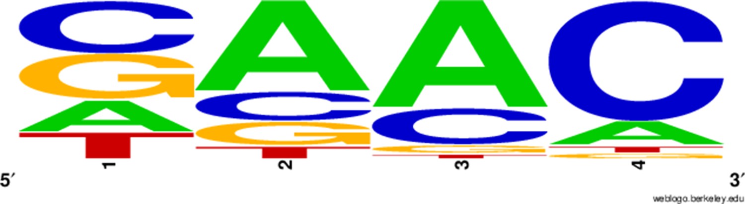
Probability logo for the four nucleotides at the 5’ end of potential protospacer sequences, generated with WebLogo; the spacer sequence starts at the right edge of the logo meaning that the reverse-complement PAM is GTT.
Figure 80
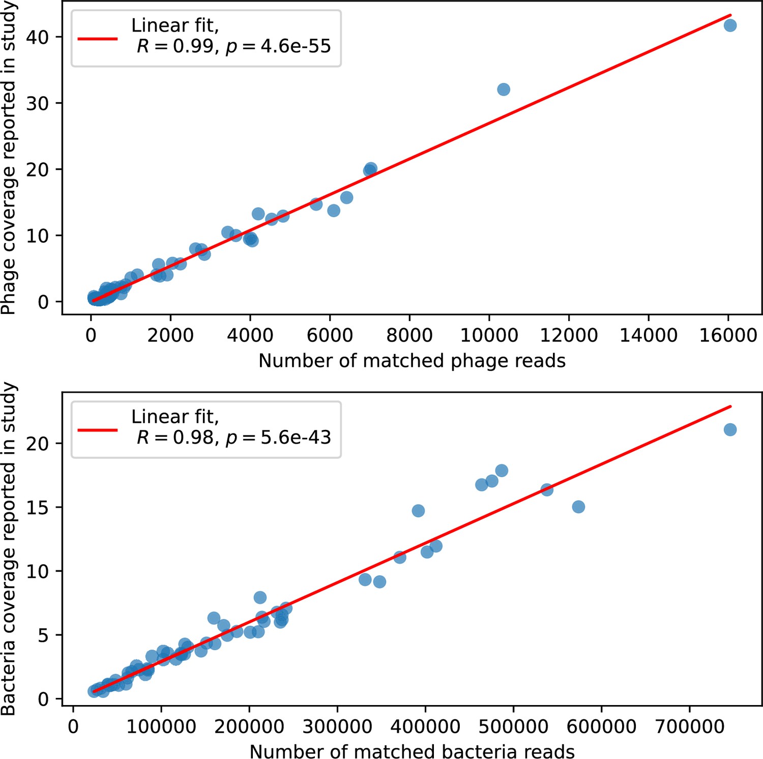
Phage genome (top) and bacteria genome (bottom) coverage, digitized from Figure 2D of Guerrero et al., 2021a vs. number of reads assigned to phage or bacteria from our analysis.
Each marker is a separate time point.
Figure 81
Abundance over time for the 20 largest bacteria clones (top) and phage clones (bottom) over time for data from Guerrero et al., 2021a.
The left panels show absolute counts, and the right panels show fractional abundance for the included types. None of the top types are shared between phage and bacteria.
Figure 82
Number of shared spacer types between bacteria and phage (top left), ratio of the number of phage types to the number of bacteria types (top right), number of bacteria types (bottom left), and number of phage types (bottom right) as a function of the sampling date for data we analysed from Guerrero et al., 2021a.
Colours indicate different similarity grouping thresholds. Spacer counts include wild-type spacers, and protospacers are included only if they possess a perfect PAM. Data is summed over CRISPR1 and CRISPR2.
Figure 83
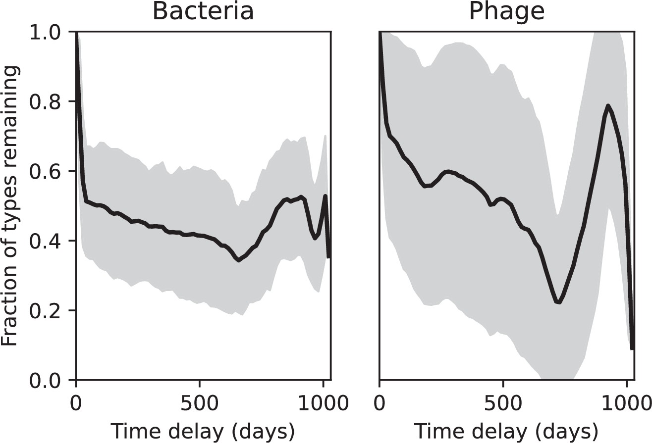
Fraction of spacer types (left) and protospacer types (right) remaining as a function of time delay, averaged over the entire time series from Guerrero et al., 2021a.
Types are grouped with an 85% similarity threshold. The grey shaded region is the standard deviation across averaged data.
Figure 84
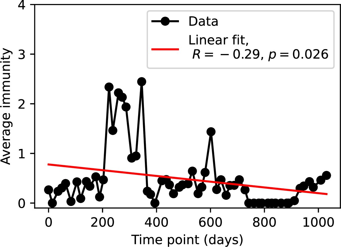
Average immunity at each time point in the time series.
Raw values cannot be larger than 1, but plotted values are multiplied by 1956, the average number of protospacers with the GTT PAM from the phage DC-56 and DS-92 genomes, yielding some values larger than 1.
Figure 85
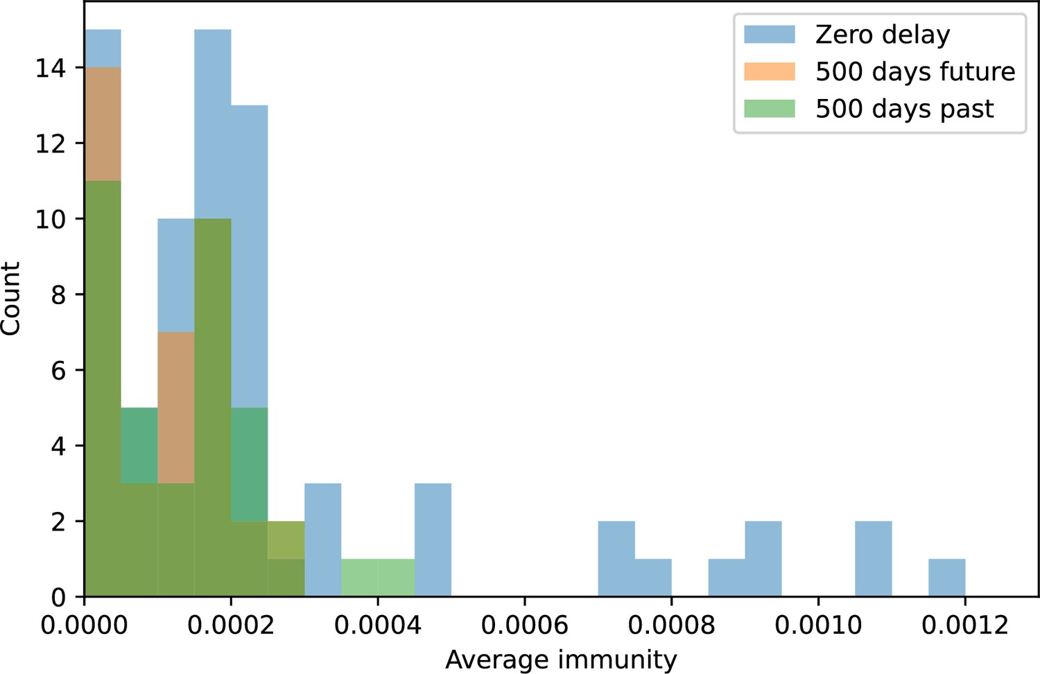
Distribution of average immunity values at zero time shift (blue) and at 500 days time shift for future phages (orange) and 500 days time shift for past phages (green).
Figure 86

p-values for the Wilcoxon signed-rank test comparing the average immunity at zero time shift with all other time shifts.
Bacteria immunity against past phages is generally not significantly lower than bacterial immunity against current phages (blue), while bacterial immunity against future phages is significantly lower than immunity against current phages for almost all time shifts (orange). The time shifts are not symmetric; bacterial overlap with past phages is not necessarily the same as phage overlap with future bacteria and vice versa. The number of points that are available to compare decreases as the time shifts get larger (black dashed line).
Figure 87
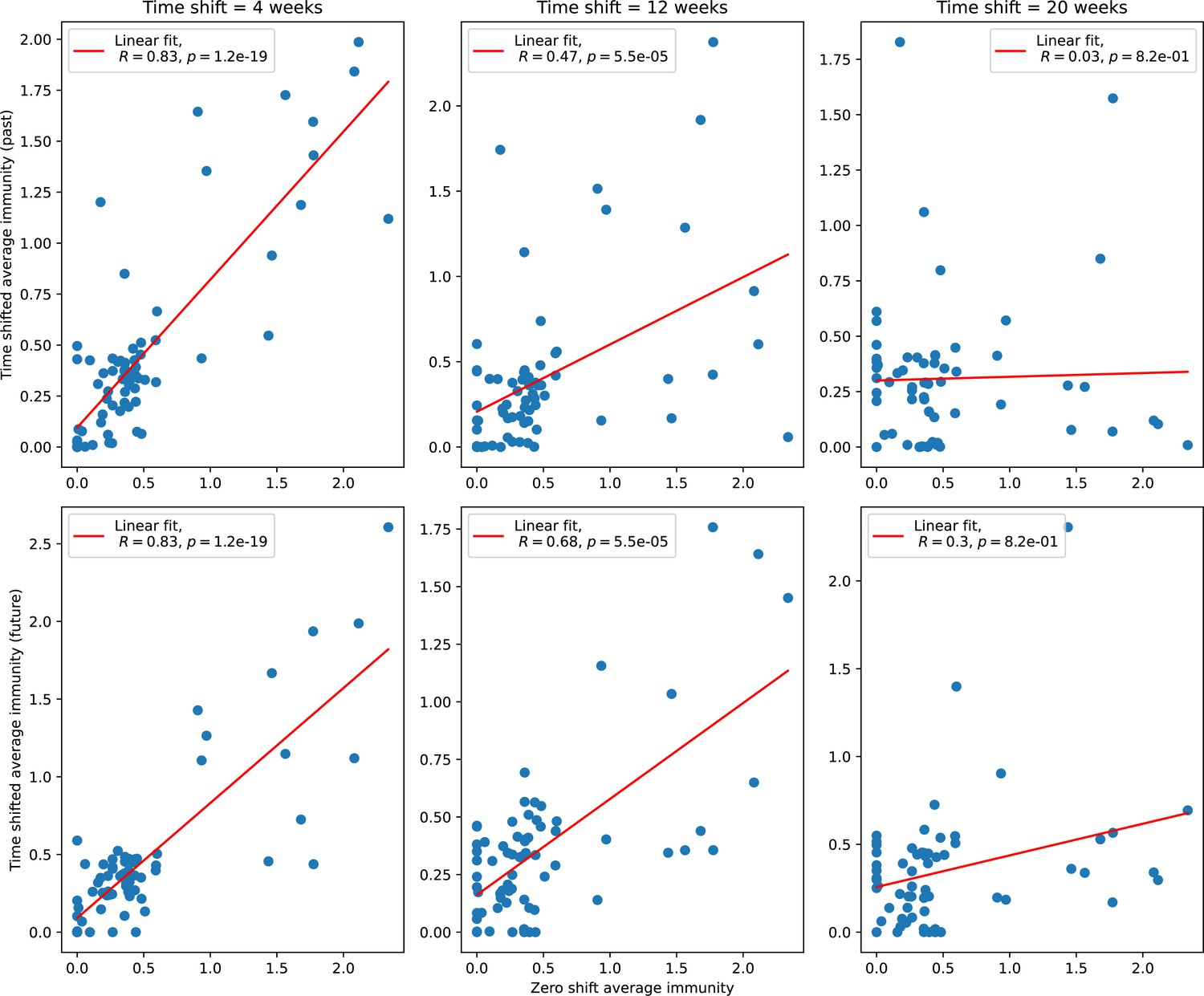
Time-shifted average immunity for each time point as a function of the zero-shift average immunity of that data point for shifts comparing past phages (top row) and future phages (bottom row).
Figure 88

Phage (top) and bacteria (bottom) population size vs. average immunity calculated with data from Guerrero et al., 2021a.
Protospacers are included if they have a perfect PAM, and all wild-type spacers are included. Spacers and protospacers are grouped with an 85% similarity threshold. Colours from blue to yellow indicate increasing time.
Appendix 2—figure 1

Diversity vs. (left), (centre), and (right) for .
The dependence of diversity is not very well predicted even by the full numerical solution, but for mutation rate and spacer effectiveness the approximate solutions do pretty well in this regime. The simulation data increase in diversity as a function of spacer acquisition probability actually goes more like .
Appendix 2—figure 2

Approximate predictions for diversity in our coevolution model (blue) or a simple model with mutation but no coevolution (orange).
(A) Predicted diversity as a function of spacer acquisition probability in our coevolution model as given by Equation 111 for , , and (blue). Predicted diversity in the non-coevolving model as given by with (orange). The low- limit is . The high- limit is a series expansion in for giving . (B) Fold change in diversity as a function of fold change in mutation rate or spacer acquisition probability under the simple approximation that (blue) and (orange).
Appendix 2—figure 3
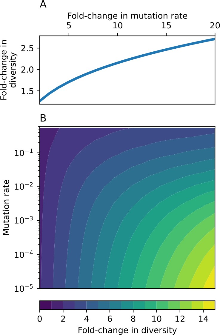
Fold change in diversity (number of species) as a function of mutation rate and , the fold change in mutation rate.
(A) Fold change in diversity as a function of fold change in mutation rate in the coevolution model: diversity increases by approximately a factor of , independent of mutation rate (solid line). (B) Fold change in diversity as a function of both mutation rate and fold change in mutation rate in the model without coevolution.
Appendix 3—figure 1
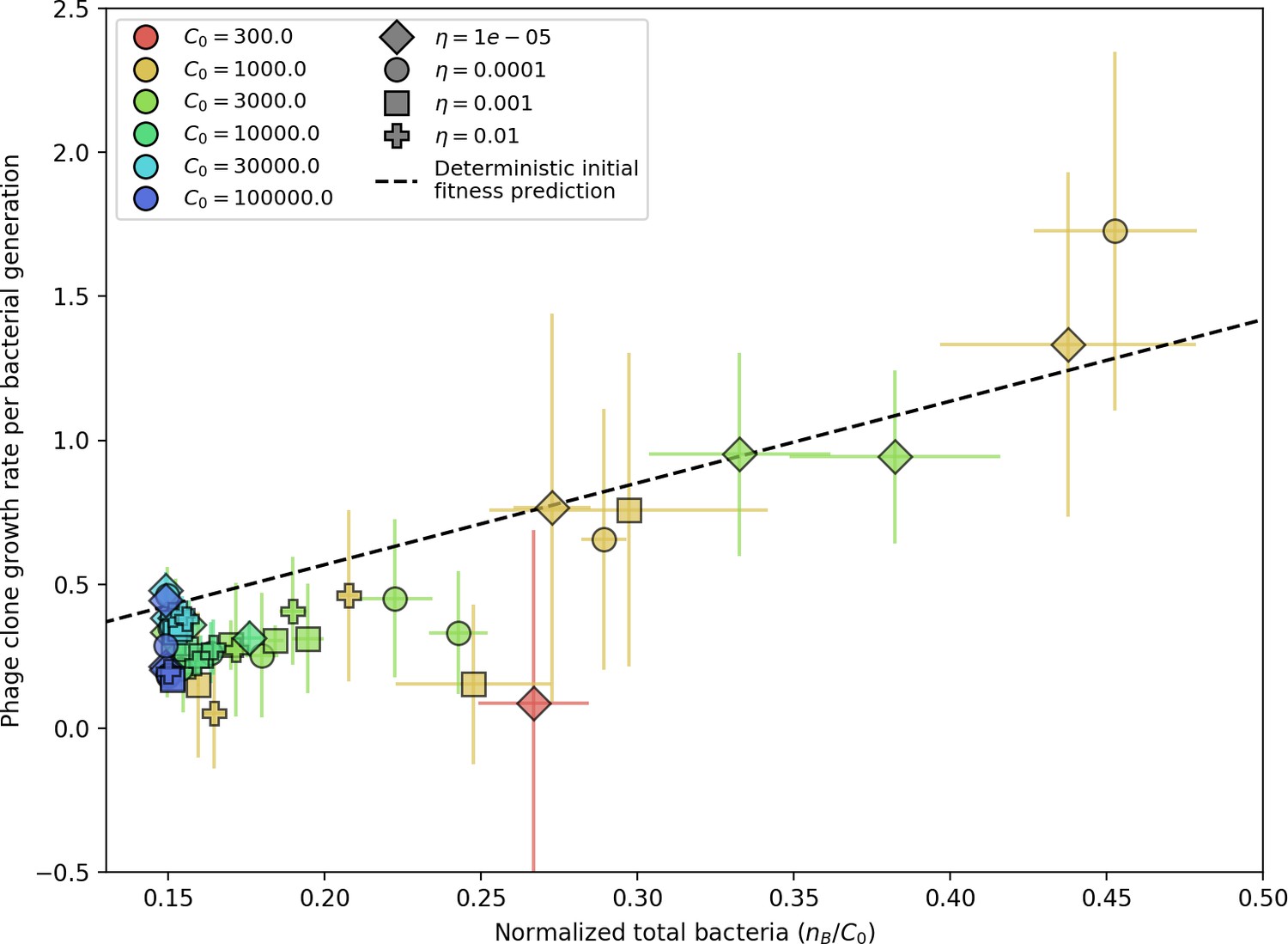
Phage clone initial growth rate vs. total bacteria normalized by the initial nutrient concentration C0.
Phage clone growth rate is as defined in Figure 3—figure supplement 1; for each simulation, the average phage clone growth rate is the derivative of the average phage clone size, averaged across all trajectories after steady state; plotted points and error bars are the average across three or more simulations. The phage initial fitness depends slightly on the phage mutation rate (mutants decrease the growth rate of a particular phage clone), but this dependence is slight enough that all mutation rates collapse onto the theoretical line. Here we plot data with . The phage clone initial growth rate also does not depend on or because new phage mutants see the bacteria population as if it did not have any CRISPR immunity. The theoretical initial phage clone growth rate is given by Equation 122. The effective lower bound of is set by the steady-state population size without CRISPR immunity: .
Appendix 3—figure 2
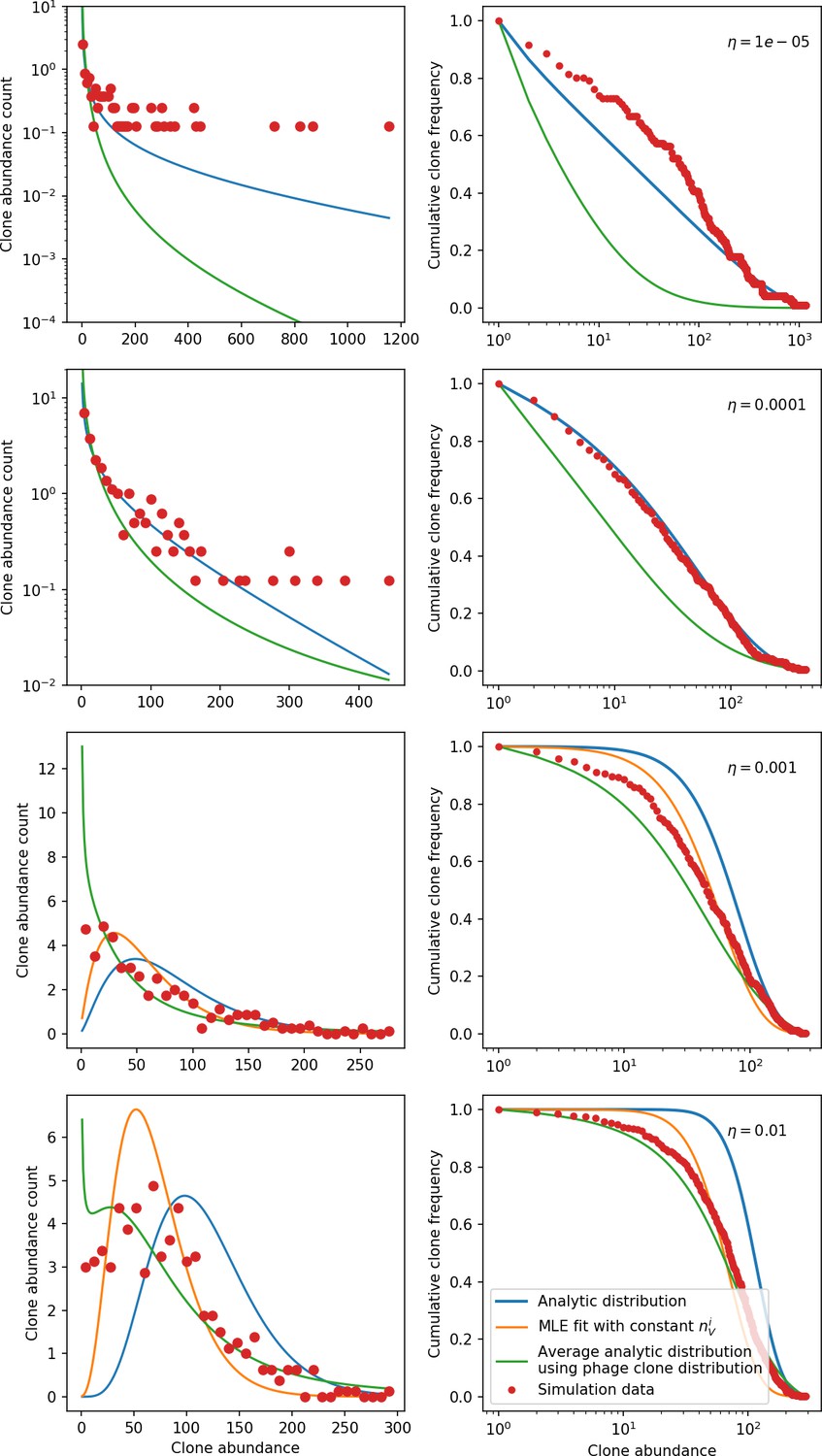
Clone size histograms (left) and cumulative distributions (right) for four different values of the spacer acquisition probability .
In all simulations, , , and . We sample 30 evenly spaced time points between 2000 and 10,000 bacterial generations and combine the clone sizes at each of the sampled points to create the clone size distributions plotted. Solid lines show three different theoretical solutions. The solid blue line is given by Equation 133 with all population quantities predicted from solving the system of Equations 13–17 with given by Equation 32 and . The solid orange line is given by Equation 133, with the value determined by maximum likelihood estimation (MLE) to give the best fit to the data. For the two largest values of , the value of returned by the MLE fit is smaller than the theoretical value of , while for the two smallest values of the MLE value of is larger. For large enough values of , the bacteria clone death rate is smaller than the birth rate which violates the assumptions used to derive Equation 133. This happens for the MLE fit at the two smallest values and hence no MLE solution is plotted. The solid green line is an average distribution calculated by solving Equation 133 at each observed large phage clone size and averaging across the distribution of clone sizes; i.e. . The large phage clone distribution is given by Equation 28.
Appendix 3—figure 3
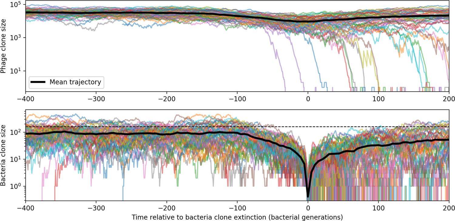
Bacteria and phage clone trajectories aligned to the time at which bacteria trajectories go extinct.
Bacteria trajectories are included if they reach size given by Equation 25 and all corresponding phage trajectories are plotted. In this simulation , , , and .
Appendix 3—figure 4
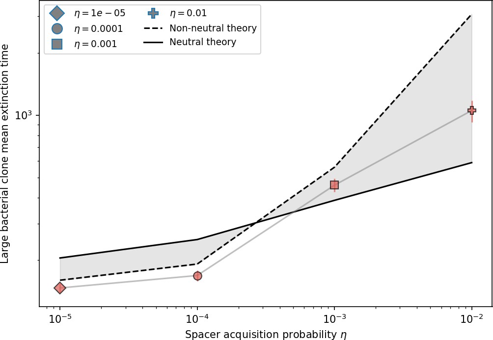
Mean time to extinction for bacterial clones after reaching size as a function of for , , and .
The solid line is given by Equation 139 with , and the dashed line is given by numerically solving Equation 137.
Appendix 3—figure 5
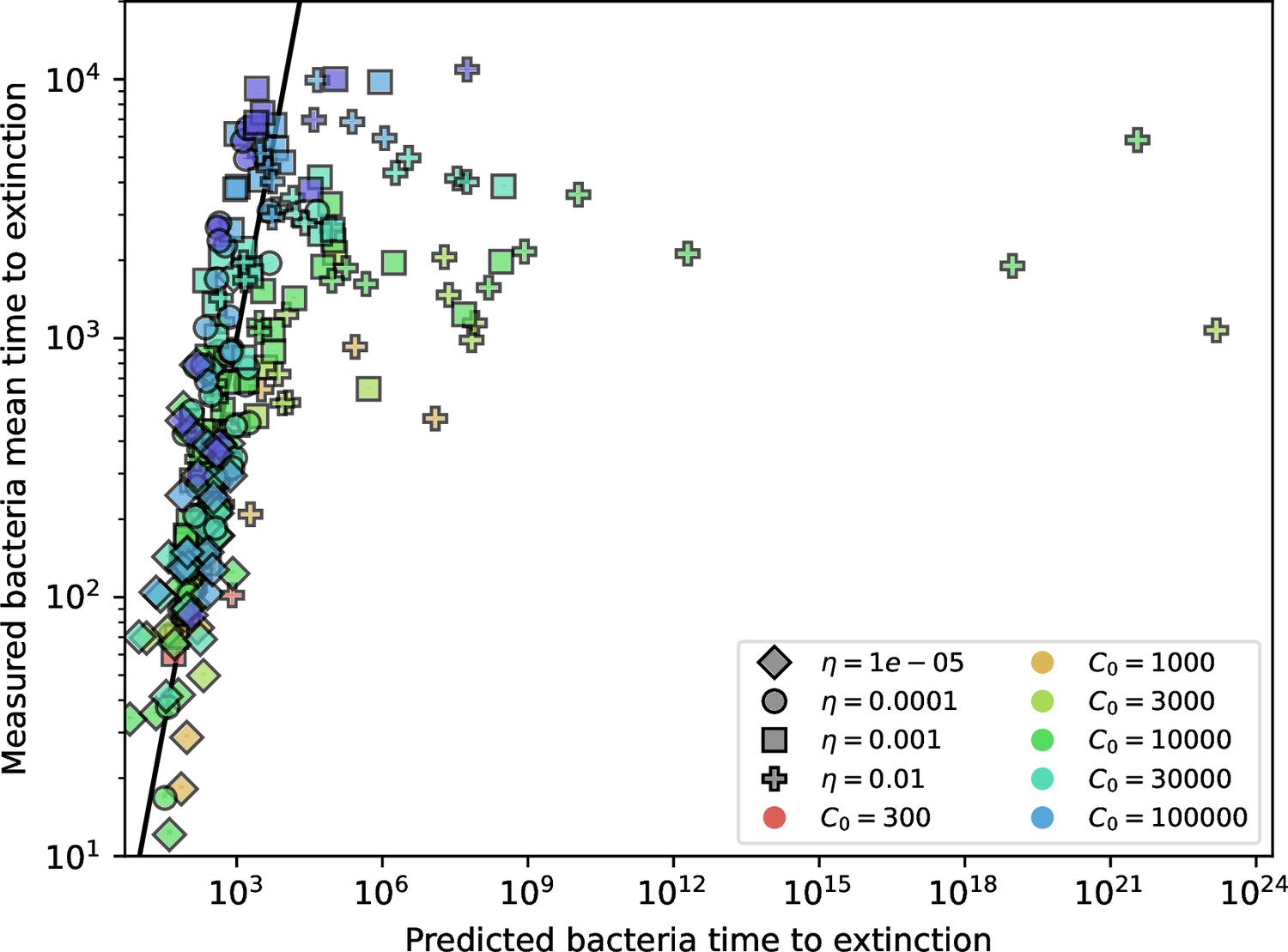
Predicted bacteria clone time to extinction with drift.
Measured vs. predicted mean time to extinction for bacterial clones after reaching size . The predicted time to extinction is the solution with drift, given by numerically solving Equation 167.
Appendix 3—figure 6
Approximations for bacteria clone extinction.
Measured mean time to extinction for large bacterial clones vs. three successively more aggressive analytic approximations for the mean time to extinction. (A) The predicted time to extinction is given by taking a series expansion in and keeping terms to 1st order. (B) A series expansion in and keeping the 0th order term () only. (C) Series expansion in and and keeping the 0th order term only (Equation 143).
Appendix 3—figure 7
Approximations for bacteria clone extinction as a function of mean clone size.
Bacteria extinction time as a function of mean clone size. Large bacteria clone mean time to extinction as a function of , where is measured from simulations and is the total bacteria population size. This parameter combination describes the trend in both phage and bacteria extinction reasonably well at large values of (bottom panels). The solid line is given by Equation 145 without the $1 + \ln m$ term.
Appendix 3—figure 8
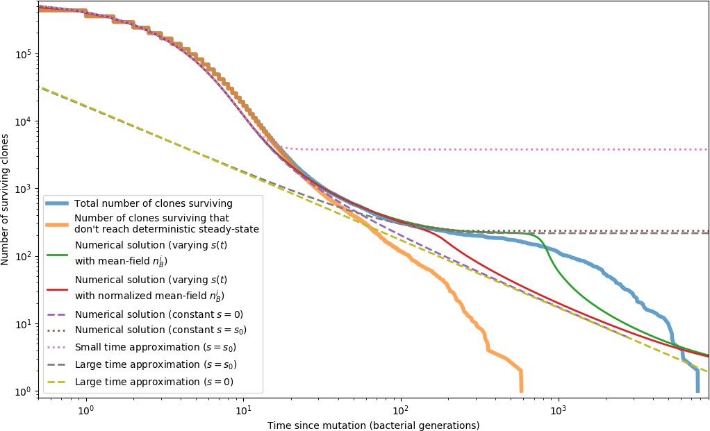
Phage clone extinction times and theoretical predictions for a simulation with parameters .
Time zero for each trajectory is the time at which that clone arose by mutation. All simulation trajectories are plotted in blue, and a subset of trajectories that do not reach a size of as given by Equation 26 are plotted in orange. Trajectories that do not become established by this definition go extinct more quickly than ones that do. All other curves are theoretical predictions for the extinction time. The green and red solid lines and purple and brown dashed lines show a numerical solution to Equation 153 with different values for . The remaining dashed lines are a small time approximation given by Equation 163, and a large time approximation given by Equation 156 with either or . All of these predictions agree with the simulation data in different regimes; none accurately captures the entire timecourse of extinctions.
Appendix 3—figure 9
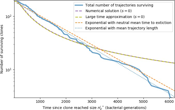
Large clone extinction times from a simulation with parameters .
Trajectories are counted as large if the phage clone size passes , the theoretical deterministic mean phage clone size for these parameters given by Equation 26. Once a trajectory reaches , we count that point as time zero to measure the extinction time of large clones. The numerical solution is given by solving Equation 153 with (). The large time approximation is given by Equation 157. The orange dashed line gives an exponential decay prediction with the mean time to extinction given by Equation 171 with .
Appendix 3—figure 10
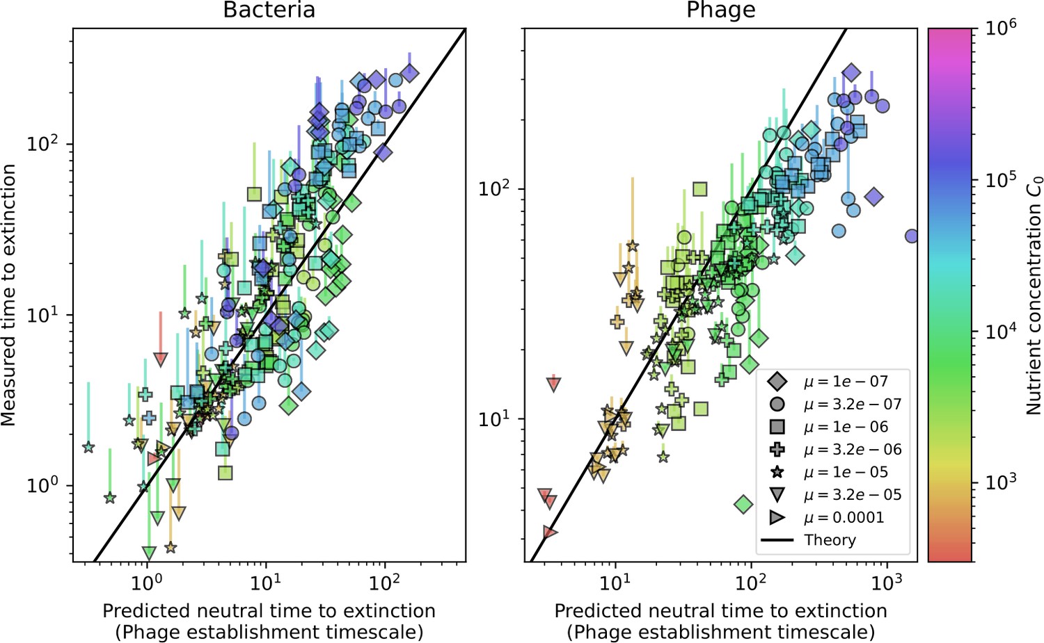
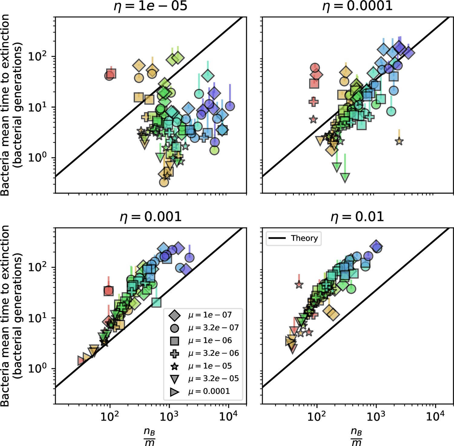
Mean time to extinction for large bacteria (left) and phage (right) clones as a function of the neutral fitness mean time to extinction prediction.
The solid black lines describe approximate analytic expressions for bacteria and phage time to extinction using a neutral fitness assumption. For bacteria, the black line solves Equation 139 using the mean bacteria and phage clone sizes. For phages, the black line solves Equation 171 using the mean phage clone size in place of .
Appendix 3—figure 11
Phage extinction time as a function of mean clone size.
Large phage clone mean time to extinction as a function of , where is measured from simulations and is the total phage population size. The solid line is given by Equation 172 without the term.
Tables
Table 1
Model reactions.
| Bacterium divides | |
| Bacterium flows out | |
| Phage flows out | |
| Nutrients flow in | |
| Nutrients flow out | |
| Interaction, phage wins, | |
| probability of mutuant phages | |
| Interaction, bacterium survives | |
| Interaction, bacterium survives and acquires a spacer | |
| Interaction, phage wins, | |
| probability of mutant phages | |
| Interaction, bacterium survives | |
| Bacterium loses spacer |
Table 2
Simulation length.
| C0 | Simulation length (bacterial generations) | Steady-state start time () |
|---|---|---|
| 300 | 10,000 | 2000 |
| 1000 | 10,000 | 2000 |
| 3000 | 10,000 | 2000 |
| 10,000 | 10,000 | 2000 |
| 30,000 | 15,000 | 3000 |
| 100,000 | 20,000 | 4000 |
| 300,000 | 25,000 | 5000 |
| 1,000,000 | 30,000 | 6000 |
Table 3
Model parameters.
| Parameter | Description | Value |
|---|---|---|
| Bacterial doubling time | 41.7 min | |
| C0 | Inflow nutrient concentration in | 102 to 10-6 |
| Units of bacterial cell density | ||
| Phage adsorption rate | ||
| Phage burst size | 170 | |
| Chemostat flow rate | ||
| Probability of phage success | 0.02 | |
| for bacteria without spacers | ||
| Spacer effectiveness | 0.1 to 0.95 | |
| Rate of spacer loss | ||
| Probability of spacer acquisition | 10-5 to 10-2 | |
| Phage mutation rate per base per generation | 10-8 to 10-4 | |
| Phage protospacer length in nucleotides | 30 |
-
Parameter values are as above unless otherwise indicated. Representative values estimated for Streptococcus thermophilus bacteria in lab conditions.
Table 4
approximations.
| ≤0.01 | 0.01 to 0.05 | 0.05 to 0.1 | 0.1 to 0.5 | 0.5 to 1 | |
|---|---|---|---|---|---|
| 10-5 to10-4 | |||||
| 10-4 to 10-2 | |||||
-
Note: the drop- solution also works for below for all values of (since ), but the solution is simpler and so preferred for the very low range.
Additional files
Download links
A two-part list of links to download the article, or parts of the article, in various formats.
Downloads (link to download the article as PDF)
Open citations (links to open the citations from this article in various online reference manager services)
Cite this article (links to download the citations from this article in formats compatible with various reference manager tools)
Dynamics of immune memory and learning in bacterial communities
eLife 12:e81692.
https://doi.org/10.7554/eLife.81692


