The mini-IDLE 3D biomimetic culture assay enables interrogation of mechanisms governing muscle stem cell quiescence and niche repopulation
- Institute of Biomedical Engineering, University of Toronto, Canada
- Donnelly Centre, University of Toronto, Canada
- Department of Cell and Systems Biology, University of Toronto, Canada
- Department of Cell, Developmental, and Regenerative Biology, Icahn School of Medicine at Mount Sinai, United States
- Black Family Stem Cell Institute, Icahn School of Medicine at Mount Sinai, United States
- Graduate School of Biomedical Sciences, Icahn School of Medicine at Mount Sinai, United States
- Université Claude Bernard Lyon 1, CNRS UMR 5261, INSERM U1315, Institut NeuroMyoGène - Pathophysiology and Genetics of Neuron and Muscle, France
Figures
Figure 1 with 2 supplements
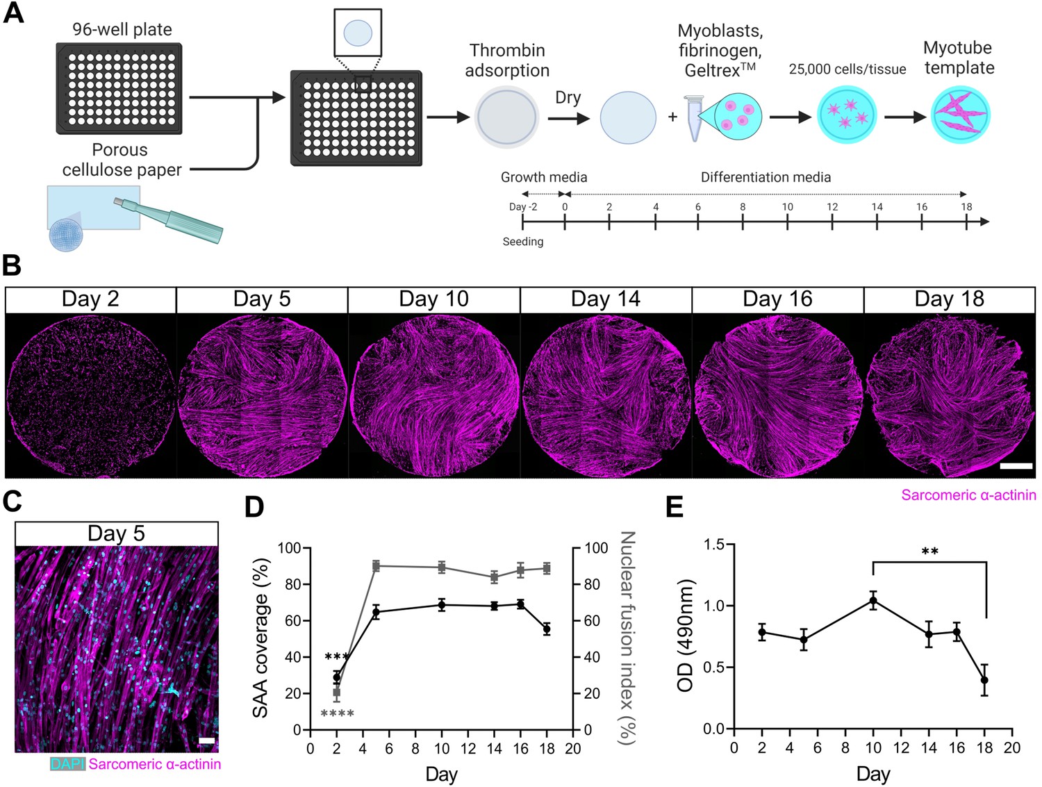
A three-dimensional (3D) murine skeletal muscle myotube template with a 96-well footprint.
(A) Schematic overview of the strategy used to generate myotube templates with an associated timeline for downstream culture (made with BioRender). (B) Representative confocal stitched images of myotube templates labelled for sarcomeric α-actinin (SAA; magenta) at days 2, 5, 10, 14, 16, and 18 of culture. Scale bar, 1 mm. (C) Representative confocal image of myotubes at day 5 labelled with DAPI (cyan) and SAA (magenta). Scale bar, 50 µm. (D) Quantification of SAA area coverage (left axis; black line) and nuclear fusion index (right axis; grey line) of myotube templates at days 2, 5, 10, 14, 16, and 18 of culture. n=9–16 across N=3–6 independent biological replicates. Graph displays mean ± s.e.m.; one-way ANOVA with Tukey’s post-test, minimum ***p=0.002 (SAA coverage), ****p˂0.0001 (nuclear fusion index). (E) Optical density (OD) at 490 nm of media after myotube template incubation with MTS assay reagent on days 2, 5, 10, 14, 16, and 18 of culture. n=9–12 across N=3–4 independent biological replicates. Graph displays mean ± s.e.m.; one-way ANOVA with Tukey’s post-test, **p=0.0033. Raw data available in Figure 1—source data 1.
-
Figure 1—source data 1
Raw data for Figure 1.
Data for subpanels separated into tabs.
- https://cdn.elifesciences.org/articles/81738/elife-81738-fig1-data1-v2.xlsx
Figure 1—figure supplement 1
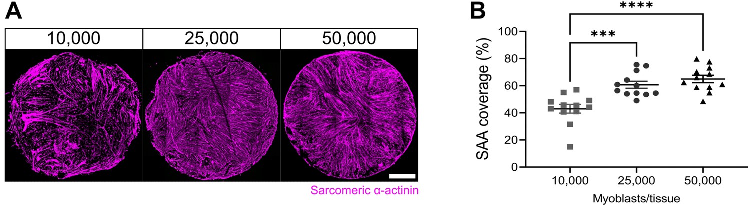
Optimization of cell seeding density.
(A) Representative confocal stitched images of myotube templates labelled for sarcomeric α-actinin (SAA; magenta) at day 5 using 10,000, 25,000, or 50,000 myoblasts per tissue. Scale bar, 1 mm. (B) Quantification of SAA area coverage of myotube templates at day 5 of differentiation using 10,000, 25,000, or 50,000 cells. n=12 across N=3 independent biological replicates. Graph displays technical replicates with mean ± s.e.m.; one-way ANOVA with Tukey’s post-test, ***p=0.0003, ****p˂0.0001. Raw data available in Figure 1—figure supplement 1—source data 1.
-
Figure 1—figure supplement 1—source data 1
Raw data for Figure 1—figure supplement 1.
Data for subpanels separated into tabs.
- https://cdn.elifesciences.org/articles/81738/elife-81738-fig1-figsupp1-data1-v2.xlsx
Figure 1—figure supplement 2
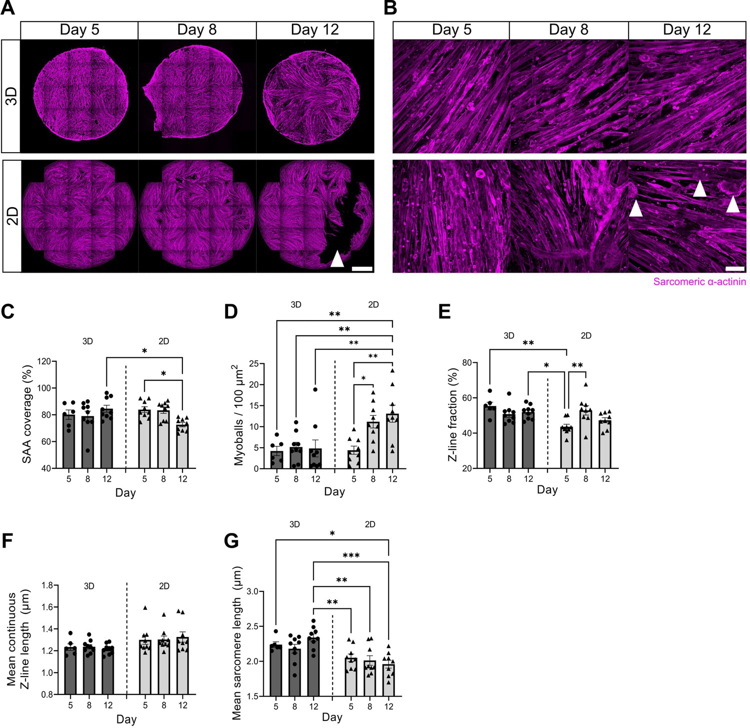
Accelerated maturity and prolonged culture of myotube templates over two-dimensional (2D) monolayers.
(A) Low- and (B) high-magnification representative confocal images of myotube templates labelled for sarcomeric α-actinin (SAA) (magenta) at days 5, 8 and 12 of differentiation in a 3D gel (top row) vs. 2D monolayer (bottom row). In (A), white arrow shows myotube detachment site in 2D cultures and scale bar, 1 mm. In (B), white arrows show detached myotubes, termed ‘myoballs’ and scale bar, 50 µm. (C) Bar graph displaying SAA area coverage at days 5, 8, and 12 of differentiation in 3D vs. 2D. n=6–9 across N=3 independent biological replicates, graph displays mean ± s.e.m. with the individual technical replicates; one-way ANOVA with Tukey’s post-test, *p=0.0264, 0.0429. (D) Quantification of myoballs per 100 µm2 at days 5, 8, and 12 of differentiation in 3D vs. 2D. n=6–9 across N=3 independent biological replicates, graph displays mean ± s.e.m. with the individual technical replicates; one-way ANOVA with Tukey’s post-test, *p=0.0343, **p=0.0081, 0.0081, 0.0053, 0.0029. (E) Bar graph showing fraction of α-actinin skeleton classified as Z-lines by actin guided segmentation (Z-line fraction) at days 5, 8 and 12 of differentiation in 3D vs. 2D. n=6–9 across N=3 independent biological replicates, graph displays mean ± s.e.m. with the individual technical replicates; one-way ANOVA with Tukey’s post-test, *p=0.0226, **p=0.0020, 0.0081. (F) Bar graph with mean continuous Z-line length at days 5, 8, and 12 of differentiation in 3D vs. 2D. n=6–9 across N=3 independent biological replicates, graph displays mean ± s.e.m. with the individual technical replicates; one-way ANOVA with Tukey’s post-test, ns. (G) Bar graph of mean sarcomere length at days 5, 8, and 12 of differentiation in 3D vs. 2D. n=6–9 across N=3 independent biological replicates, graph displays mean ± s.e.m. with the individual technical replicates; one-way ANOVA with Tukey’s post-test, *p=0.0356, **p=0.0097, 0.0025, ***p=0.0003. Raw data available in Figure 1—figure supplement 2—source data 1.
-
Figure 1—figure supplement 2—source data 1
Raw data for Figure 1—figure supplement 2.
Data for subpanels separated into tabs.
- https://cdn.elifesciences.org/articles/81738/elife-81738-fig1-figsupp2-data1-v2.xlsx
Figure 2 with 1 supplement
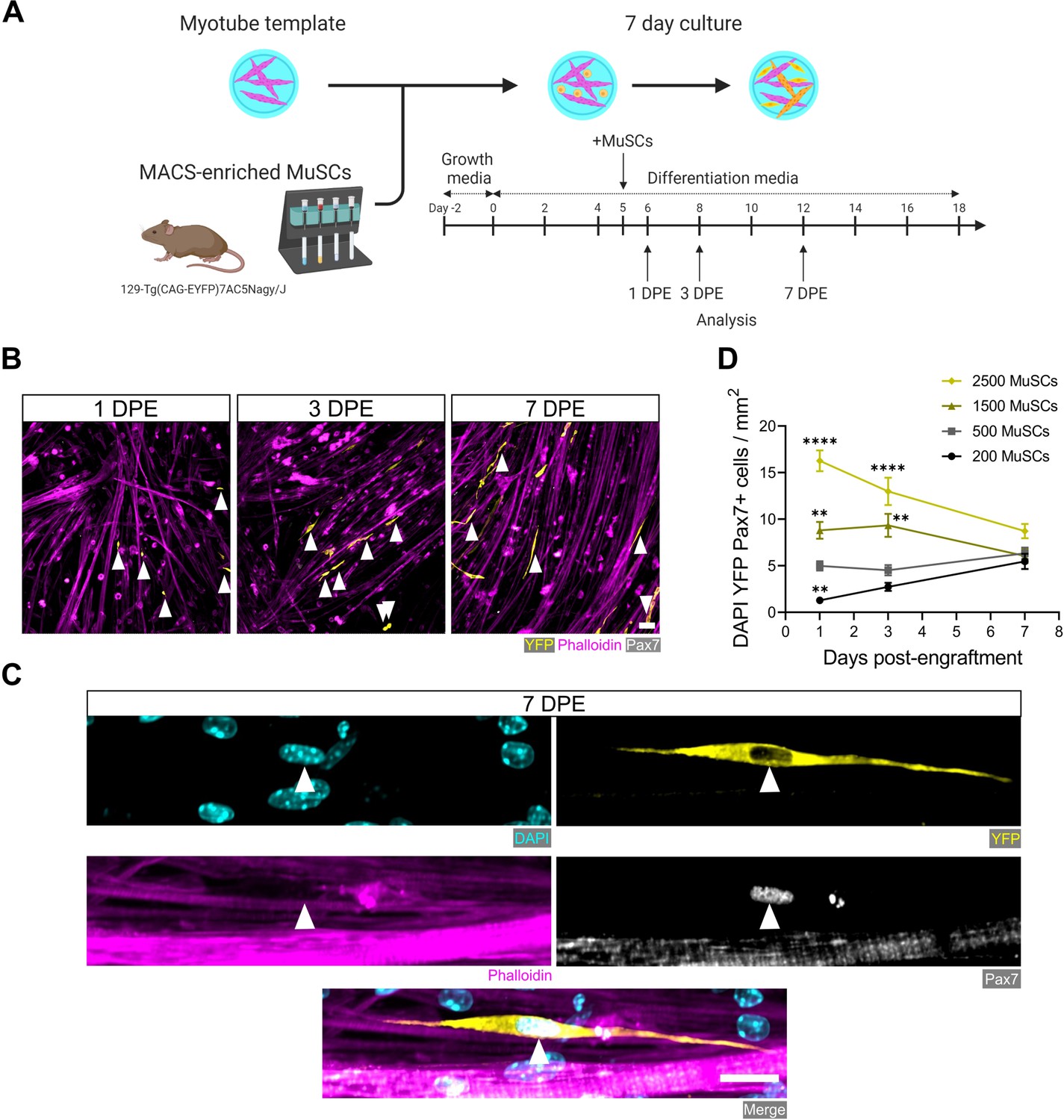
Engrafted muscle stem cells (MuSCs) persist in myotube template cultures and achieve a steady-state population density.
(A) Schematic overview of the engraftment of freshly isolated MuSCs and the timeline for downstream analysis (made with BioRender). (B) Representative confocal images of myotube templates (phalloidin: magenta) with engrafted MuSCs (YFP: yellow, Pax7: white, white arrows) at 1, 3, and 7 days post-engraftment (DPE). Scale bar, 50 µm. (C) Representative confocal image of a donor MuSC (DAPI: cyan, YFP: yellow, Pax7: white) indicated with a white arrow, and myotubes (phalloidin: magenta) at 7 DPE. Scale bar, 20 µm. (D) Quantification of mononuclear DAPI+YFP+Pax7+ cell density per mm2 at 1, 3, and 7 DPE across different starting MuSC engraftment numbers (200, 500, 1500, and 2500). n=9–15 across N=3–5 independent biological replicates. Graph displays mean ± s.e.m.; one-way ANOVA with Dunnet’s test for each individual timepoint comparing against the 500 MuSC condition, **p=0.0025, 0.0051, 0.0029, ****p˂0.0001. Raw data available in Figure 2—source data 1.
-
Figure 2—source data 1
Raw data for Figure 2.
Data for subpanels separated into tabs.
- https://cdn.elifesciences.org/articles/81738/elife-81738-fig2-data1-v2.xlsx
Figure 2—figure supplement 1
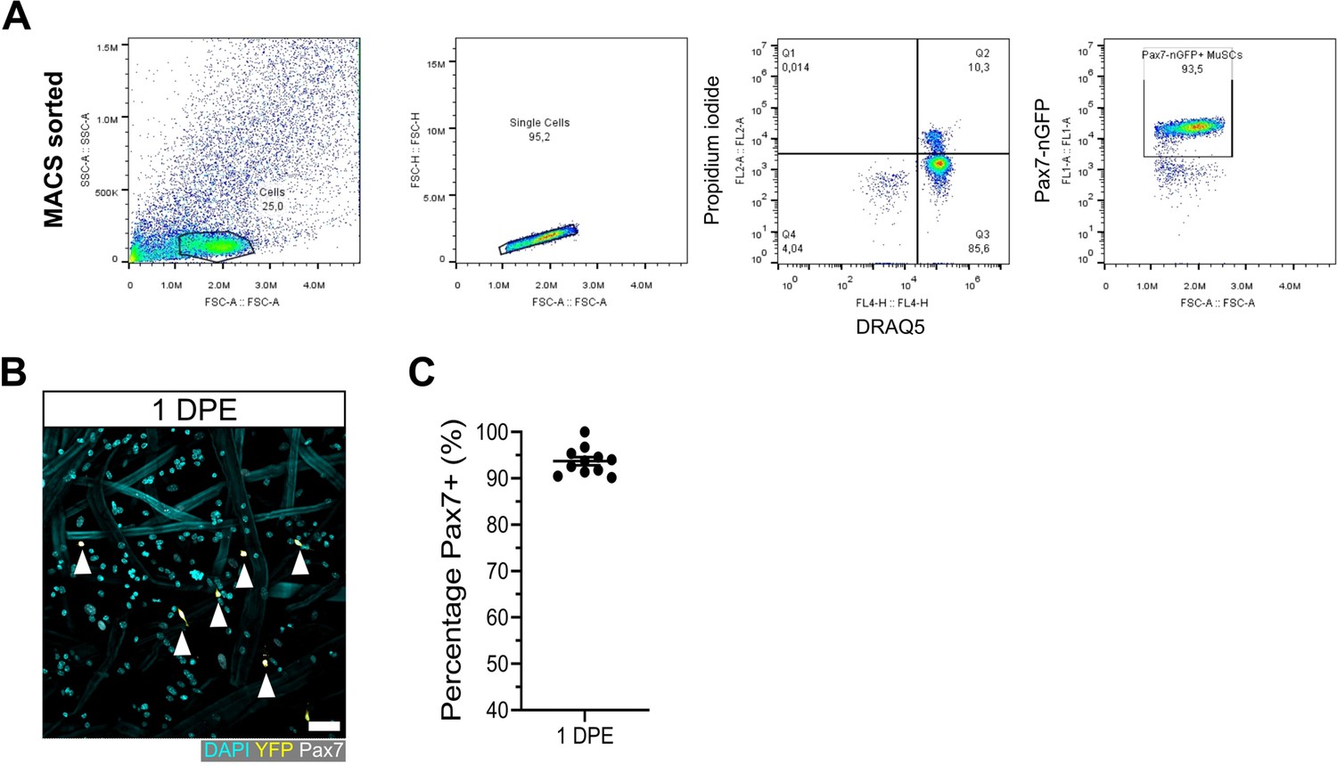
Population purity in magnetic-activated cell sorting (MACS) isolated muscle stem cells (MuSCs).
(A) Flow cytometry gating of MuSCs enriched from the hindlimb muscles of a Pax7-nGFP mouse using the MACS-based workflow. (B) Representative confocal image of MuSCs (DAPI: cyan, YFP: yellow, Pax7: white, white arrows) at 1 day post-engraftment (DPE) onto myotube templates. Scale bar, 50 µm. (C) Quantification of the percentage Pax7+ cells in the DAPI+YFP+ population at 1 DPE after engraftment with CAG-EYFP reporter MuSCs. n=11 across N=3 independent biological replicates. Graph displays mean ± s.e.m. of technical replicates. Raw data available in Figure 2—figure supplement 1—source data 1.
-
Figure 2—figure supplement 1—source data 1
Raw data for Figure 2—figure supplement 1.
Data for subpanels separated into tabs.
- https://cdn.elifesciences.org/articles/81738/elife-81738-fig2-figsupp1-data1-v2.xlsx
Figure 3 with 3 supplements
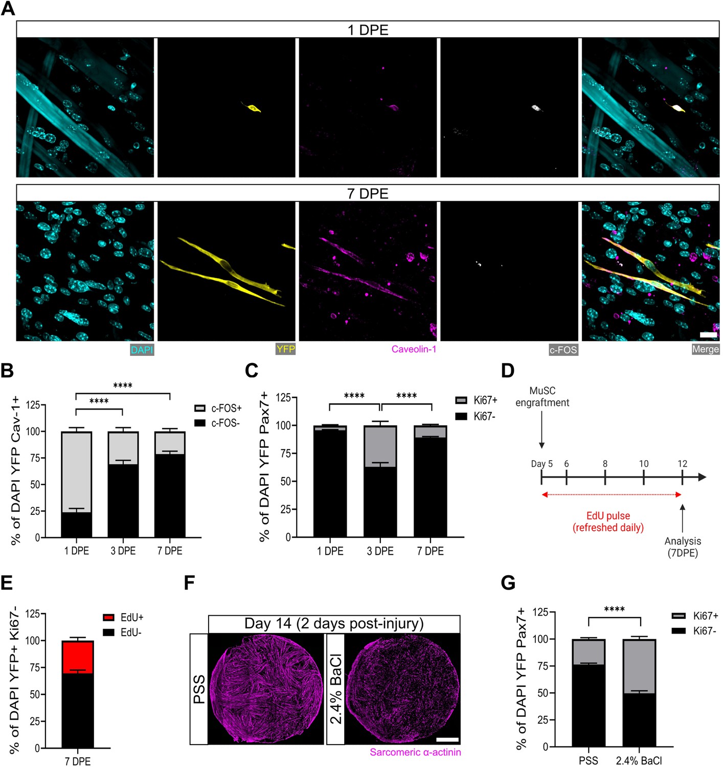
Muscle stem cells (MuSCs) engrafted within engineered muscle tissue exit cell cycle and inactivate.
(A) Representative confocal image of a mononuclear cell (DAPI: cyan) positive for YFP (yellow), caveolin-1 (magenta), and c-FOS (white) at 1 day post-engraftment (DPE) (top), and a c-FOS- cell at 7 DPE (bottom). Scale bar, 20 µm. (B) Stacked bar graph showing proportions of c-FOS ± cells at 1, 3, and 7 DPE in the DAPI+YFP+Cav-1+ population. n=9 across N=3 independent biological replicates. Graph displays mean ± s.e.m. for c-FOS+ and c-FOS-; one-way ANOVA with Tukey’s post-test comparing the FOS- proportions of each timepoint, ****p˂0.0001. (C) Stacked bar graph showing proportions of Ki67 ± cells at 1, 3, and 7 DPE in the DAPI+YFP+Pax7+ population. n=10–11 across N=3–4 independent biological replicates. Graph displays mean ± s.e.m. for Ki67+ and Ki67-; one-way ANOVA with Tukey’s post-test comparing the Ki67- proportions of each timepoint, ****p˂0.000.1. (D) Timeline of EdU/Ki67 co-labelling experiment (made with BioRender). (E) Stacked bar graph showing proportions of EdU ± cells at 7 DPE in the DAPI+YFP+Ki67- mononuclear cell population. n=15 across N=5 independent biological replicates. Graph displays mean ± s.e.m. for EdU+ and EdU-. (F) Representative confocal stitched images of myotube templates (sarcomeric α-actinin (SAA): magenta) 2 days after a 4 hr exposure to the physiological salt solution (PSS) control or a 2.4% barium chloride (BaCl2) solution. Scale bar, 1 mm. (G) Proportion of Ki67 ± cells at 2 days post-injury (DPI) in the DAP+YFP+Pax7+ population. n=16, 18 across N=5, 6 biological replicates. Graph displays mean ± s.e.m. for Ki67+ and Ki67-; unpaired t-test of the Ki67- proportions of both conditions, ****p˂0.0001. Raw data available in Figure 3—source data 1.
-
Figure 3—source data 1
Raw data for Figure 3.
Data for subpanels separated into tabs.
- https://cdn.elifesciences.org/articles/81738/elife-81738-fig3-data1-v2.xlsx
Figure 3—figure supplement 1
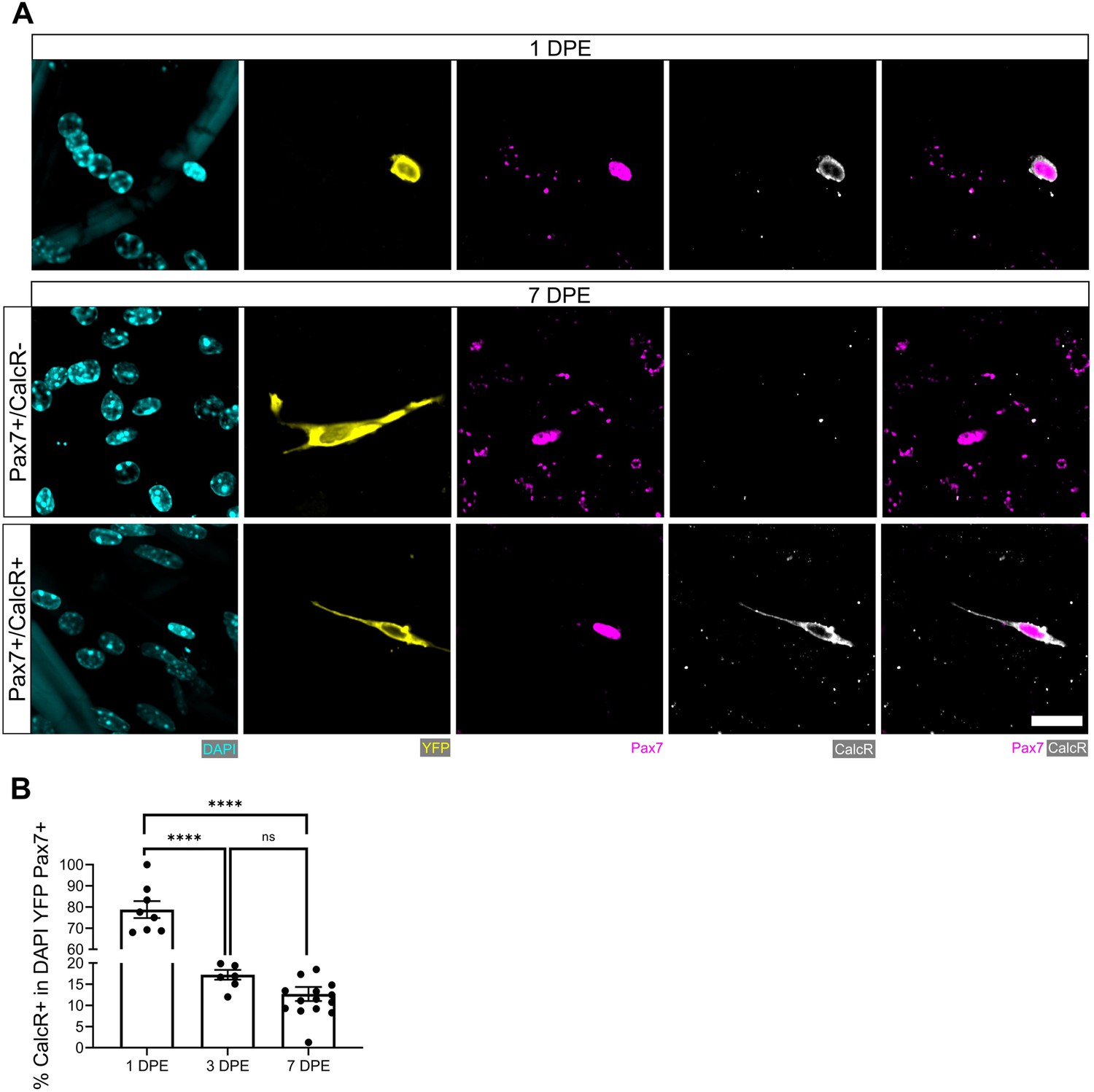
Persistent CalcR+ population amongst Pax7+ donor cell population at 7 days post-engraftment (DPE).
(A) Representative confocal images of a Pax7+ (magenta) donor cells (yellow) at 1 DPE (top) and 7 DPE (middle and bottom) immunostained for calcitonin receptor (CalcR: white) and counterstained with DAPI (cyan). Scale bar, 20 µm. (B) Bar graph showing the percentage of CalcR+ cells in the DAPI+YFP+Pax7+ mononucleated cell population at 1, 3, and 7 DPE. n=7–15 across N=3–5 independent biological replicates. Graph displays mean ± s.e.m. of the individual technical replicates; one-way ANOVA with Tukey’s post-test, ****p˂0.0001. Raw data available in Figure 3—figure supplement 1—source data 1.
-
Figure 3—figure supplement 1—source data 1
Raw data for Figure 3—figure supplement 1.
Data for subpanels separated into tabs.
- https://cdn.elifesciences.org/articles/81738/elife-81738-fig3-figsupp1-data1-v2.xlsx
Figure 3—figure supplement 2

Characterization of barium chloride-induced injury.
(A) Quantification of sarcomeric α-actinin (SAA) coverage on day 12 of differentiation, and 2 days (day 14) after a physiological salt solution (PSS; carrier control) or 2.4% BaCl2 exposure. n=7–9 across N=3 independent biological replicates. Graph displays mean ± s.e.m. with individual technical replicates; one-way ANOVA with Tukey’s post-test, ****p˂0.0001. (B) Quantification of DAPI+YFP+Pax7+ mononucleated cell density on day 12 of differentiation, and 2 days (day 14) after a PSS or 2.4% BaCl2 exposure. n=6–9 across N=2–3 independent biological replicates. Graph displays mean ± s.e.m. with individual technical replicates; one-way ANOVA, non-significant (ns). Raw data available in Figure 3—figure supplement 2—source data 1.
-
Figure 3—figure supplement 2—source data 1
Raw data for Figure 3—figure supplement 2.
Data for subpanels separated into tabs.
- https://cdn.elifesciences.org/articles/81738/elife-81738-fig3-figsupp2-data1-v2.xlsx
Figure 3—figure supplement 3
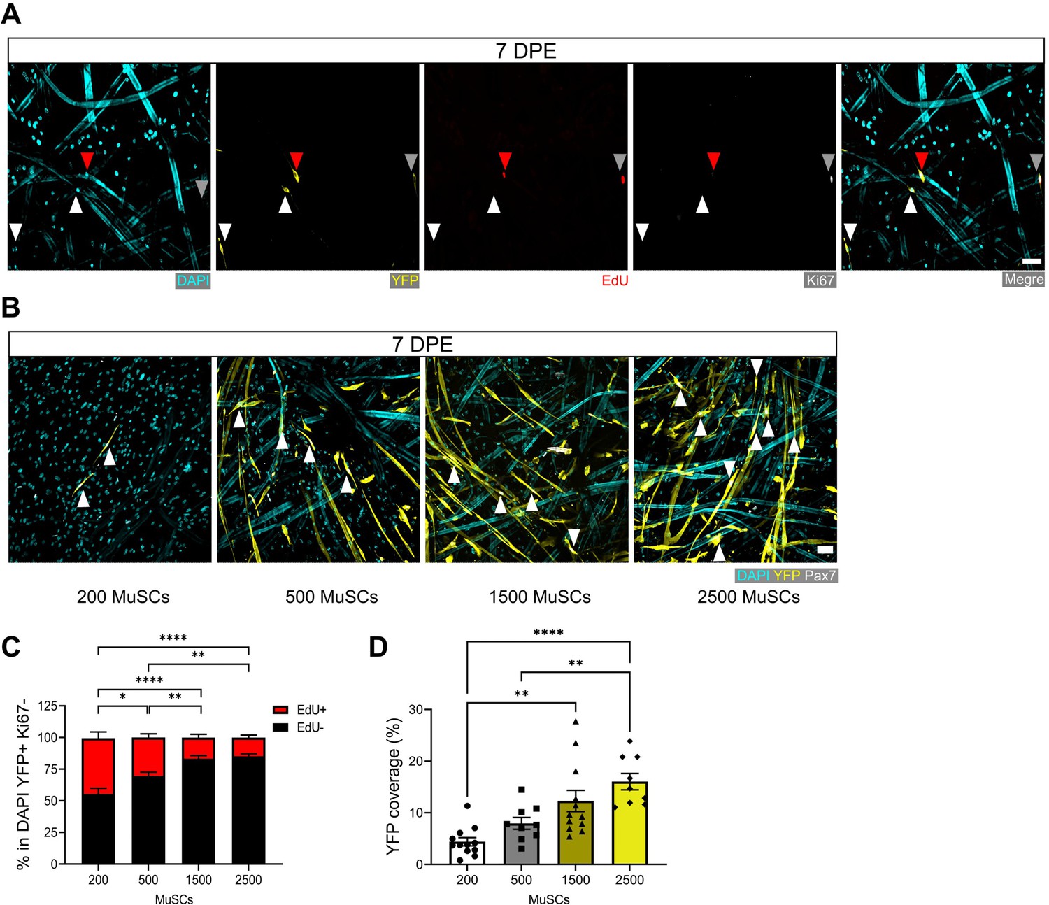
Regulation of muscle stem cell (MuSC) pool size in myotube template cultures.
(A) Representative confocal image of YFP+ (yellow) mononucleate donor cells at 7 days post-engraftment (DPE) co-labelled for EdU (red), Ki67 (white), and nuclei (DAPI: cyan), to visualize EdU+Ki67- (red arrow), EdU+Ki67+ (white, grey arrow), and EdU-Ki67- (white arrows) populations. Scale bar, 50 µm. (B) Representative confocal images of tissues at 7 DPE initially seeded with 200, 500, 1500, or 2500 MuSCs (DAPI: cyan, YFP: yellow, Pax7: white, white arrows). Scale bar, 50 µm. (C) Proportion of EdU ± cells at 7 DPE in the DAPI+YFP+Ki67- population across different starting MuSC engraftment numbers (200, 500, 1500, or 2500). n=10–16 across N=3–5 independent biological replicates. Graph displays mean ± s.e.m. for EdU+ and EdU-; one-way ANOVA with Tukey’s post-test comparing the EdU- proportions of each condition, *p=0.0102, **p=0.0063, 0.0026, ****p˂0.0001. (D) Quantification of tissue area covered by YFP signal at 7 DPE when engrafted with 200, 500, 1500, or 2500 MuSCs. n=9–12 across N=3–4 independent biological replicates. Graph displays mean ± s.e.m. with individual technical replicates; one-way ANOVA with Tukey’s post-test, **p=0.0019, 0.0066, ****p˂0.0001. Raw data available in Figure 3—figure supplement 3—source data 1.
-
Figure 3—figure supplement 3—source data 1
Raw data for Figure 3—figure supplement 3.
Data for subpanels separated into tabs.
- https://cdn.elifesciences.org/articles/81738/elife-81738-fig3-figsupp3-data1-v2.xlsx
Figure 4 with 1 supplement
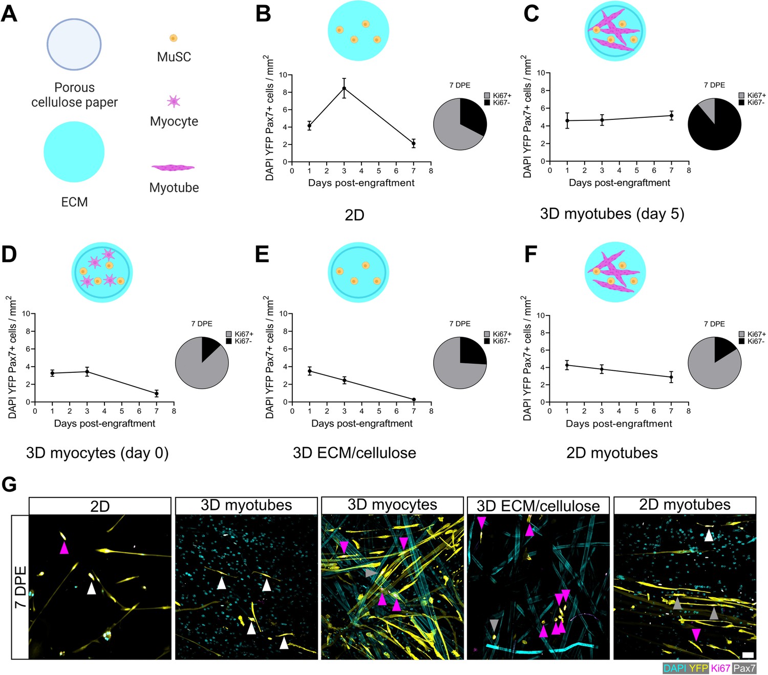
Permissive culture conditions for a persistent muscle stem cell (MuSC) population in vitro.
(A) Key for figure icons. (B–F) Line graphs of mononucleated DAPI+YFP+Pax7+ cell density at 1, 3, and 7 days post-engraftment (DPE) (left) and pie charts showing the proportion of Ki67 ± cells at 7 DPE (right) for cells seeded into a two-dimensional (2D) microwell with a Geltrex coating (B), engrafted into 3D myotube templates on day 5 (C) vs. day 0 (D) of differentiation. Additional comparisons include engraftment into a 3D cellulose-reinforced extracellular matrix (ECM) hydrogel on day 5 (E), or onto a 2D monolayer of myotubes with a Geltrex undercoating on day 5 of differentiation (F). n=6–15 from N=2–3 independent biological replicates. Graphs display mean ± s.e.m. (G) Representative confocal images of YFP+ (yellow) donor cells (DAPI: cyan) at 7 DPE engrafted in 2D, 3D with myotubes (day 5), 3D with myocytes (day 0), 3D with cellulose-reinforced ECM or with a 2D monolayer of myotubes. Cells are also labelled for Ki67 (magenta) and Pax7 (white) where Ki67-Pax7+ cells are indicated with white arrows, Ki67+Pax7+ with grey arrows, and Ki67+Pax7- with magenta arrows. Scale bar, 50 µm. Raw data available in Figure 4—source data 1.
-
Figure 4—source data 1
Raw data for Figure 4.
Data for subpanels separated into tabs.
- https://cdn.elifesciences.org/articles/81738/elife-81738-fig4-data1-v2.xlsx
Figure 4—figure supplement 1
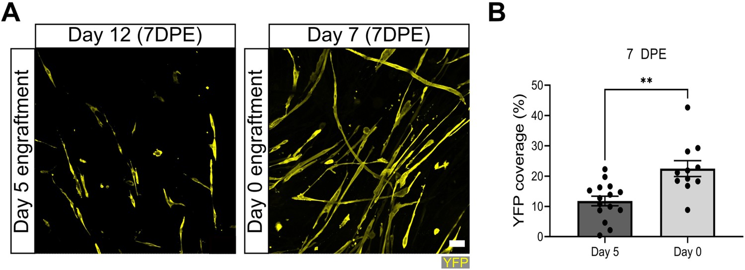
Increased YFP coverage when muscle stem cells (MuSCs) engrafted on day 0 of myotube template differentiation.
(A) Representative confocal images of tissues engrafted with 500 MuSCs at day 0 or day 5 of myotube template differentiation, fixed at 7 days post-engraftment (DPE) (i.e. days 7 and 12 of differentiation), and immunolabelled for YFP (yellow). Scale bar, 50 µm. (B) Quantification of percentage of tissue area covered by YFP signal at 7 DPE when 500 MuSCs are engrafted on day 0 vs. day 5. n=11, 15 from N=4, 5 independent biological replicates. Graph displays mean ± s.e.m. with individual technical replicates; unpaired t-test, **p=0.0012. Raw data available in Figure 4—figure supplement 1—source data 1.
-
Figure 4—figure supplement 1—source data 1
Raw data for Figure 4—figure supplement 1.
Data for subpanels separated into tabs.
- https://cdn.elifesciences.org/articles/81738/elife-81738-fig4-figsupp1-data1-v2.xlsx
Figure 5 with 5 supplements
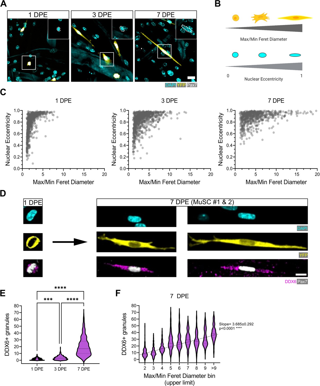
Morphological evolution of engrafted muscle stem cells (MuSCs).
(A) Representative confocal images of MuSCs (DAPI: cyan, YFP: yellow, Pax7: white) with distinct morphological features at 1, 3, and 7 days post-engraftment (DPE). Insets highlight nuclear morphology with a white dotted outline. Scale bar, 20 µm. (B) Schematic demonstrating the morphological features quantified using CellProfiler (made with BioRender). (C) Dot plot graphs showing individual Pax7+ donor cells and their associated max/min Feret diameter ratio and nuclear eccentricity at 1 (left), 3 (middle), and 7 DPE (right). n=916, 980, and 737 across N=3–4 biological replicates. (D) Representative confocal images of MuSCs (DAPI: cyan, YFP: yellow, Pax7: white) labelled for p54/RCK (DDX6) at 1 and 7 DPE. Scale bar, 10 µm. (E) DDX6+ granule quantification in individual MuSCs at 1, 3, and 7 DPE. n=639, 770, and 676 across N=3 independent biological replicates. Graph displays violin plot distribution; one-way ANOVA with Tukey’s post-test, ***p=0.0004, ****p˂0.0001. (F) Violin plot distribution of DDX6+ granules in individual MuSCs at 7 DPE stratified across max/min Feret diameter bins. n=737 across N=3 independent biological replicates. One-way ANOVA with test for linear trend across bins, ****p˂0.0001. Raw data available in Figure 5—source data 1.
-
Figure 5—source data 1
Raw data for Figure 5.
Data for subpanels separated into tabs.
- https://cdn.elifesciences.org/articles/81738/elife-81738-fig5-data1-v2.xlsx
Figure 5—figure supplement 1
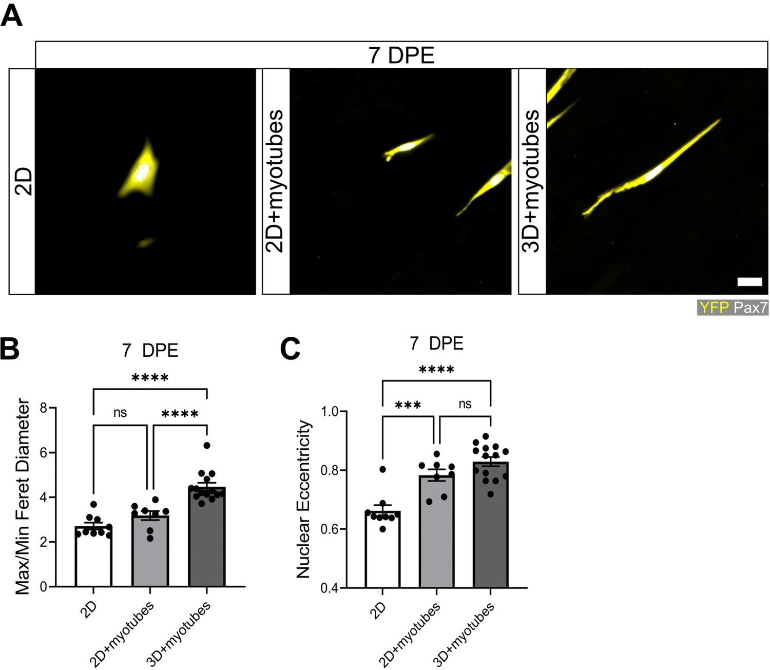
Pax7+ donor cell morphologies in two (2D) and three dimensions (3D).
(A) Representative confocal images of mononucleated donor cells (YFP:yellow; Pax7:white) after 7 days in a 2D Geltrex-coated Petri dish (left), in 2D co-culture with a myotube monolayer established on a Geltrex undercoating (middle), or engrafted into 3D myotube templates at day 5 of differentiation (right). Scale bar, 20 µm. (B) Bar plot showing the average max/min Feret diameter of the mononuclear DAPI YFP Pax7+ population at 7 days post-engraftment (DPE) engrafted in 2D, 2D myotube co-culture, or in 3D myotube template co-culture. n=8–15 across N=3 independent biological replicates. Graph displays mean ± s.e.m. with individual technical replicates; one-way ANOVA with Tukey’s post-test, ****p˂0.0001. (C) Bar plot showing the average max/min Feret diameter of the mononuclear DAPI+YFP+Pax7+ population at 7 DPE engrafted in in 2D, 2D myotube co-culture, or in 3D myotube template co-culture. n=8–15 across N=3 independent biological replicates. Graph displays mean ± s.e.m. with individual technical replicates; one-way ANOVA with Tukey’s post-test, ***p=0.0005, ****p˂0.0001. Raw data available in Figure 5—figure supplement 1—source data 1.
-
Figure 5—figure supplement 1—source data 1
Raw data for Figure 5—figure supplement 1.
Data for subpanels separated into tabs.
- https://cdn.elifesciences.org/articles/81738/elife-81738-fig5-figsupp1-data1-v2.xlsx
Figure 5—figure supplement 2
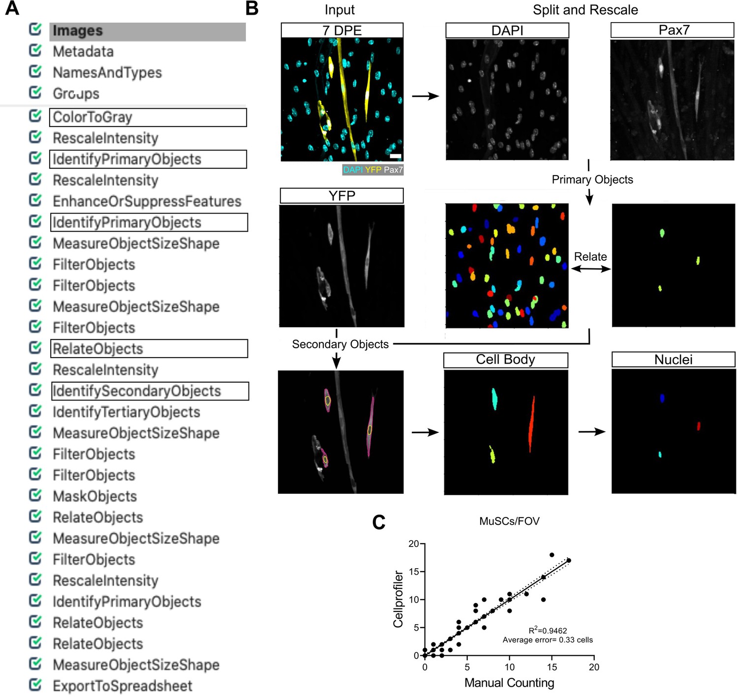
CellProfiler pipeline for muscle stem cell (MuSC) identification and characterization.
(A) Representative image of the pipeline loaded in CellProfiler. (B) Representative confocal image of mononucleated (DAPI:cyan) donor (YFP:yellow) MuSCs (Pax7:white) at 7 days post-engraftment (DPE) (white arrowheads) along with a general schematic of the CellProfiler workflow (see Materials and methods for more details). Scale bar, 20 µm. (C) Dot plot graph showing the correlation between Manual and CellProfiler counting of MuSCs in individual images (FOV). n=125 images across N=3 independent biological replicates, graph displays individual technical replicates (images) with a simple linear regression analysis (solid line) and 95% confidence intervals (dotted lines). Remark: many of the 125 data points in (C) overlap. Raw data available in Figure 5—figure supplement 2—source data 1.
-
Figure 5—figure supplement 2—source data 1
Raw data for Figure 5—figure supplement 2.
Data for subpanels separated into tabs.
- https://cdn.elifesciences.org/articles/81738/elife-81738-fig5-figsupp2-data1-v2.xlsx
Figure 5—figure supplement 3
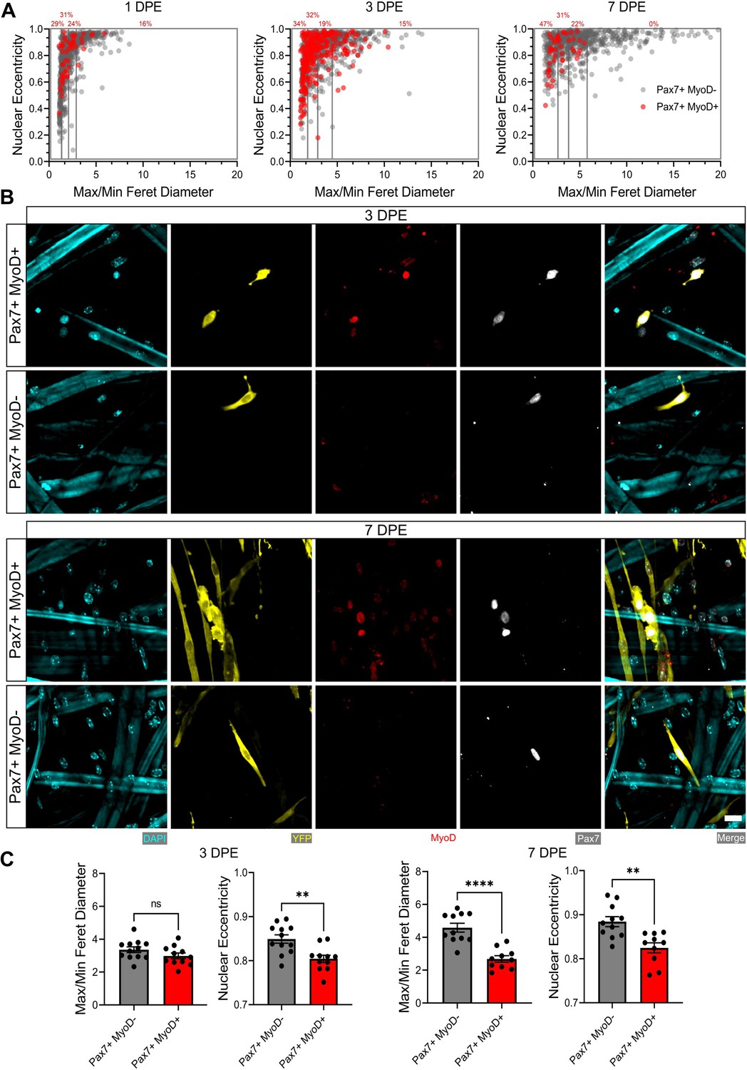
Morphological characterization of Pax7+MyoD and Pax7+MyoD+ muscle stem cells (MuSCs).
(A) Dot plot graphs showing individual Pax7+ donor cells and their associated max/min Feret diameter ratio and nuclear eccentricity at 1 (left), 3 (middle), and 7 days post-engraftment (DPE) (right) with Pax7+MyoD+ cells shown in red and Pax7+MyoD- cells in grey. Quartiles are indicated by grey boxes and the percentage of Pax7+MyoD+ cells within each quartile is written above in red. n=916, 980, and 737 across N=3–4 biological replicates also analysed in Figure 5C. (B) Representative confocal images of donor MuSCs (DAPI:cyan; YFP:yellow; Pax7:white) ±MyoD (red) at 3 (top) and 7 DPE (bottom). Scale bar, 20 µm. (C) Bar graphs showing the average max/min Feret diameter ratio and nuclear eccentricity between Pax7+MyoD- (dark grey) and Pax7+MyoD+ cells (red) at 3 (left) and 7 DPE (right). n=10–12 across N=3–4 independent technical replicates. Graphs display mean ± s.e.m. of the individual technical replicate tissues from panel A; unpaired t-test, **p=0.0021, 0.0015, ****p˂0.0001. Raw data available in Figure 5—figure supplement 3—source data 1.
-
Figure 5—figure supplement 3—source data 1
Raw data for Figure 5—figure supplement 3.
Data for subpanels separated into tabs.
- https://cdn.elifesciences.org/articles/81738/elife-81738-fig5-figsupp3-data1-v2.xlsx
Figure 5—figure supplement 4
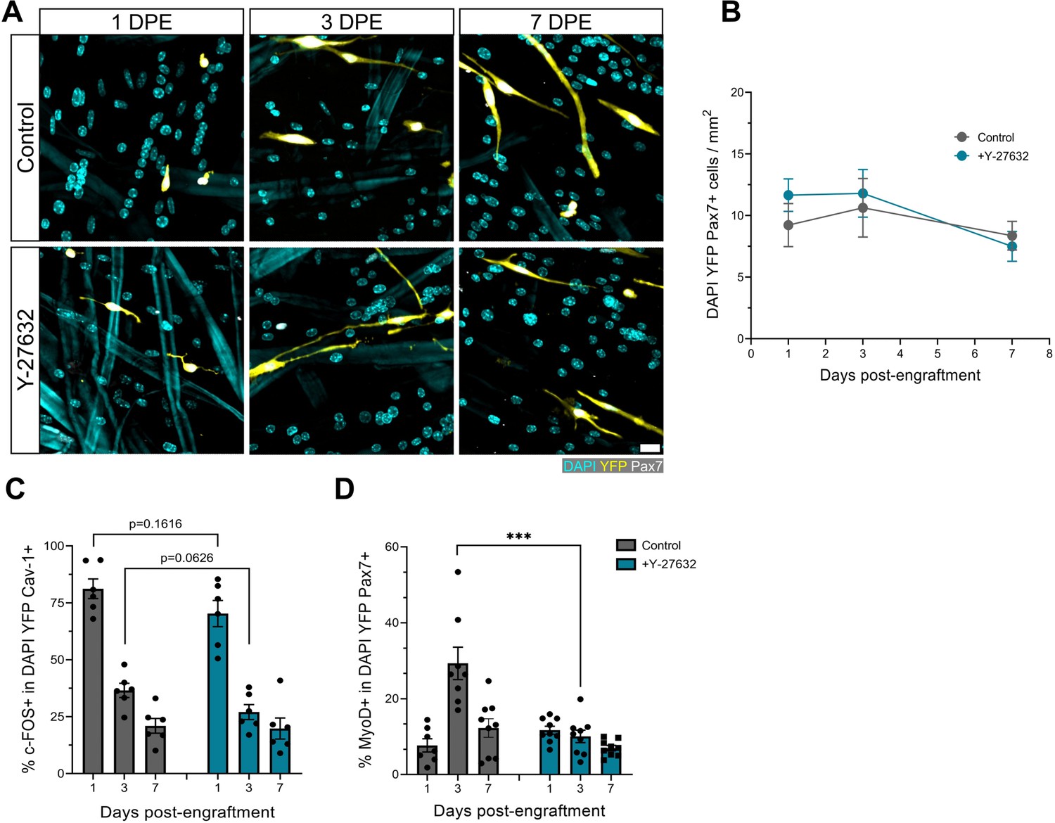
ROCK inhibition hastens muscle stem cell (MuSC) inactivation.
(A) Representative confocal images of MuSCs (DAPI: cyan, YFP: yellow, Pax7: white) at 1, 3, and 7 days post-engraftment (DPE) treated with a vehicle control or the ROCK inhibitor Y-27632. Scale bar, 20 µm. (B) Quantification of mononuclear DAPI+YFP+Pax7+ cell density per mm2 at 1, 3, and 7 DPE in the control and Y-27632 treatment condition. n=7–9 across N=3 independent biological replicates. Graph displays mean ± s.e.m.; unpaired t-tests for each individual timepoint, ns. (C) Bar plot showing the percentage of c-FOS+ cells in the mononuclear DAPI+YFP+Cav-1+ population at 1, 3, and 7 DPE in the control and Y-27632 treatment conditions. n=6 across N=2 independent biological replicates. Graph displays mean ± s.e.m. with individual technical replicates; unpaired t-tests for each individual timepoint, ns. (D) Bar plot showing the percentage of MyoD+ cells in the mononuclear DAPI+YFP+Pax7+ population at 1, 3 and 7 DPE in the control and Y-27632 treatment conditions. n=7–9 across N=3 independent biological replicates. Graph displays mean ± s.e.m. with individual technical replicates; unpaired t-tests for each individual timepoint, ***p=0.0005. Raw data available in Figure 5—figure supplement 4—source data 1.
-
Figure 5—figure supplement 4—source data 1
Raw data for Figure 5—figure supplement 4.
Data for subpanels separated into tabs.
- https://cdn.elifesciences.org/articles/81738/elife-81738-fig5-figsupp4-data1-v2.xlsx
Figure 5—figure supplement 5
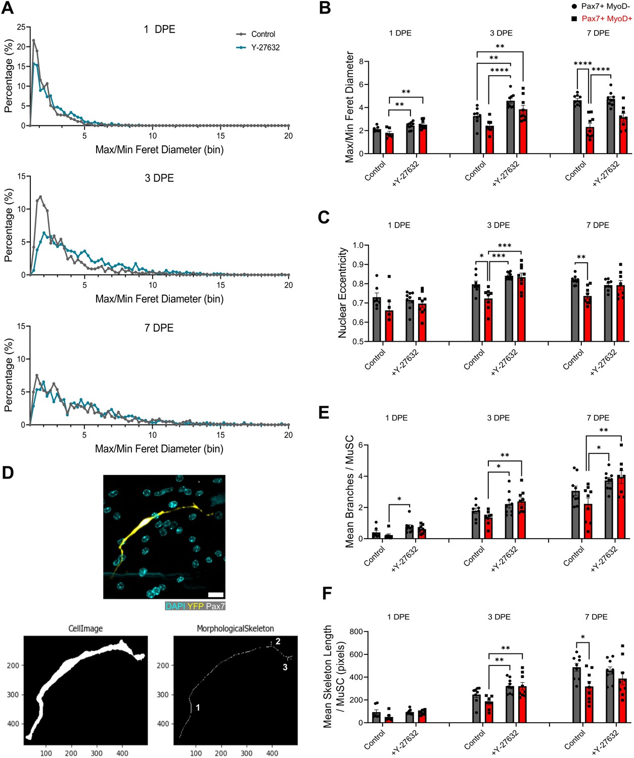
ROCK inhibition confers acquisition of quiescent-like morphologies to the Pax7+MyoD+ population.
(A) Distribution plots of individual muscle stem cell (MuSC) max/min Feret diameter bins at 1 (top), 3 (middle), and 7 days post-engraftment (DPE) (bottom) in the control and Y-27632 treatment conditions. n=666, 1255, 994, 1158, 783, 598 across N=3–4 independent biological replicates. (B) Bar plot showing the max/min Feret diameter of the Pax7+MyoD- and Pax7+MyoD+ populations at 1, 3, and 7 DPE in the control and Y-27632 treatment conditions. n=7–9 across N=3 independent biological replicates. Graph displays mean ± s.e.m. with individual technical replicates; one-way ANOVA with Tukey’s post-test within each timepoint, **p=0.0046, 0.0014, 0.0071, 0.0029, ****p˂0.0001. (C) Bar plot showing the nuclear eccentricity of the Pax7+MyoD- and Pax7+MyoD+ populations at 1, 3, and 7 DPE in the control and Y-27632 treatment conditions. n=7–9 across N=3 independent biological replicates. Graph displays mean ± s.e.m. with individual technical replicates; one-way ANOVA with Tukey’s post-test within each timepoint, *p=0.0227, **p=0.0015, ***p=0.0001, 0.0003. (D) Representative confocal image (top) of a Y-27632-treated MuSC at 3 DPE (DAPI: cyan, YFP: yellow, Pax7: white) and the CellProfiler conversion to a skeletonized image (bottom) for quantifying branch number (numbered in white) and skeleton length. Scale bar, 20 µm. (E) Bar plot showing the mean cytoplasmic branches per MuSC in the Pax7+MyoD- and Pax7+MyoD+ populations at 1, 3, and 7 DPE in the control and Y-27632 treatment conditions. N=7–9 across N=3 independent biological replicates. Graph displays mean ± s.e.m. with individual technical replicates; one-way ANOVA with Tukey’s post-test within each timepoint, *p=0.0124, 0.0336, 0.0132, **p=0.0085, 0.0053. (F) Bar plot showing the mean skeleton length in pixels per MuSC in the Pax7+MyoD- and Pax7+MyoD+ populations at 1, 3, and 7 DPE in the control and Y-27632 treatment conditions. n=7–9 across N=3 independent biological replicates. Graph displays mean ± s.e.m. with individual technical replicates; one-way ANOVA with Tukey’s post-test within each timepoint, *p=0.0360, **p=0.0021, 0.0023. Raw data available in Figure 5—figure supplement 5—source data 1.
-
Figure 5—figure supplement 5—source data 1
Raw data for Figure 5—figure supplement 5.
Data for subpanels separated into tabs.
- https://cdn.elifesciences.org/articles/81738/elife-81738-fig5-figsupp5-data1-v2.xlsx
Figure 6 with 2 supplements
Engrafted muscle stem cells (MuSCs) display quiescence and niche-related hallmarks.
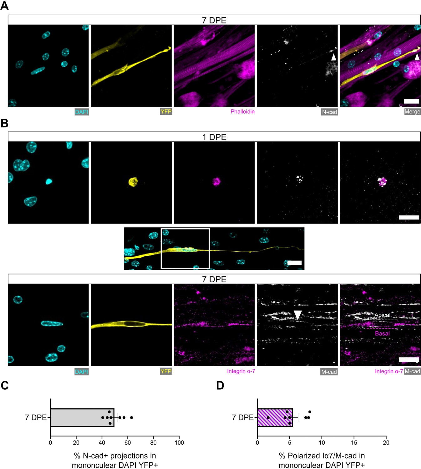
(A) Representative confocal image of a mononuclear donor cell (DAPI: cyan, YFP: yellow) with neighbouring myotubes (Phalloidin: magenta) and N-cadherin (white) localized to the tip of the donor cell projection (white arrowhead). Scale bar, 20 µm. (B) Representative confocal images of a mononuclear donor cell (DAPI: cyan, YFP: yellow) at 1 day post-engraftment (DPE) (top) and 7 DPE (middle and bottom) expressing integrin α-7 (magenta) and M-cadherin (white). Middle inset image channels are separated to produce the bottom images to highlight the polarization of integrin α-7 and M-cadherin (white arrow) to basal and apical orientations, respectively (dotted lines). Scale bars, 20 µm. (C) Bar plot showing the percentage of mononuclear DAPI+YFP+ cells with N-cadherin+ cytoplasmic projections at 7 DPE. n=8 across N=3 independent biological replicates. Graph displays mean ± s.e.m. with individual technical replicates. (D) Bar plot showing the percentage of mononuclear DAPI+YFP+ cells with polarized integrin α-7 (Iα7)/M-cadherin expression at 7 DPE. n=8 across N=3 independent biological replicates. Graph displays mean ± s.e.m. with individual technical replicates. Raw data available in Figure 6—source data 1.
-
Figure 6—source data 1
Raw data for Figure 6.
Data for subpanels separated into tabs.
- https://cdn.elifesciences.org/articles/81738/elife-81738-fig6-data1-v2.xlsx
Figure 6—figure supplement 1
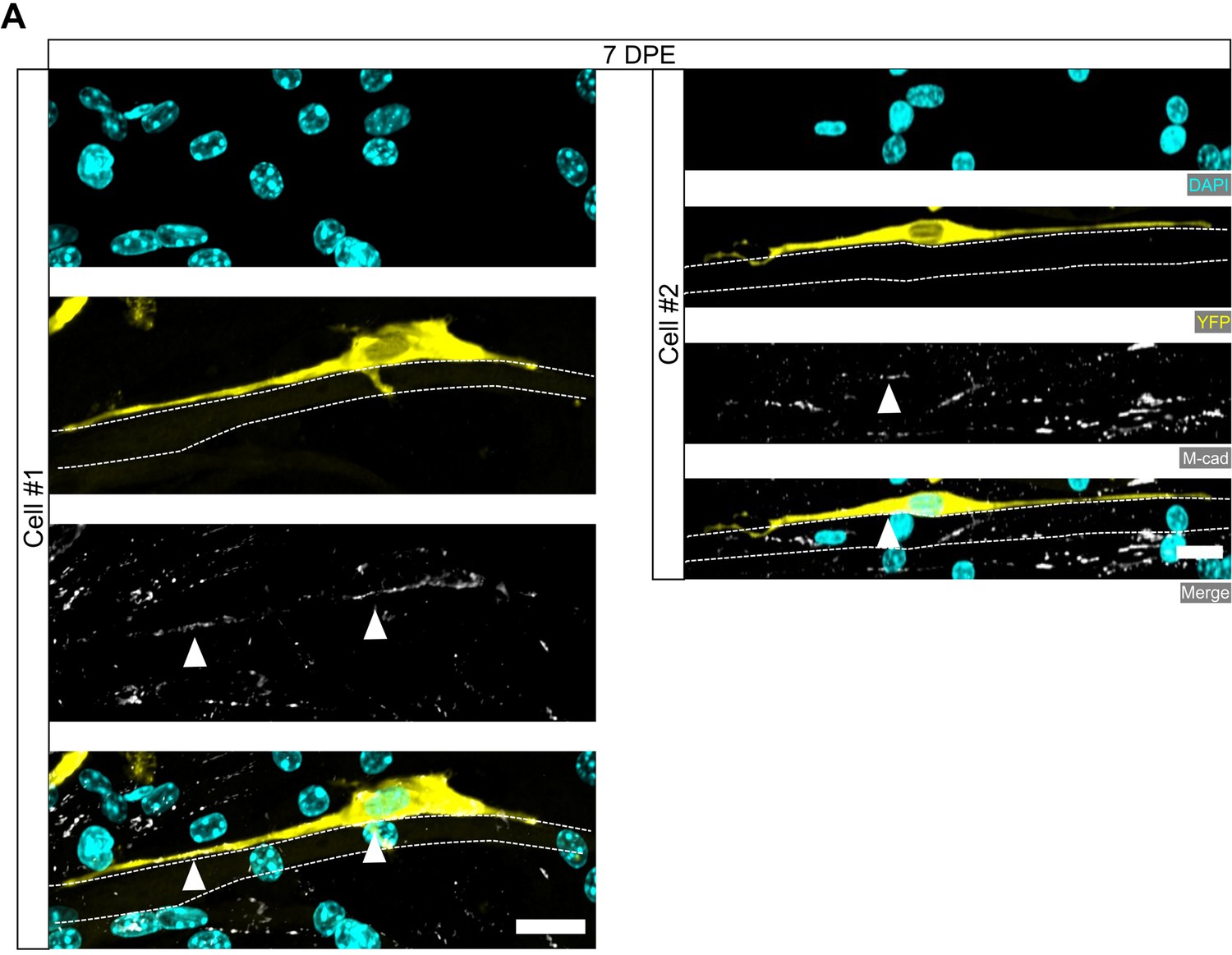
Polarized localization of M-cadherin in mononuclear donor cells at 7 days post-engraftment (DPE).
(A) Representative confocal images of two (Cell #1, left; Cell #2, right) mononucleated donor cells (DAPI: cyan; YFP: yellow) with M-cadherin (M-cad: white, white arrows) labelling restricted to the apical side. Cells are associated with myotubes that were visualized using the background signal (white dotted lines). Scale bars, 20 µm.
Figure 6—figure supplement 2
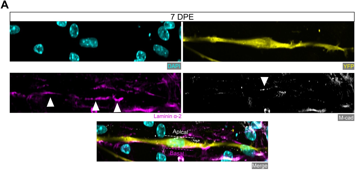
Donor cell polarization of niche markers at 7 days post-engraftment (DPE).
(A) Representative confocal image of a mononucleated donor cell (DAPI: cyan; YFP: yellow) with M-cadherin (white) immunolabelling restricted to the apical side and laminin α-2 (magenta) localized to the basal side. Scale bar, 20 µm.
Figure 7 with 2 supplements
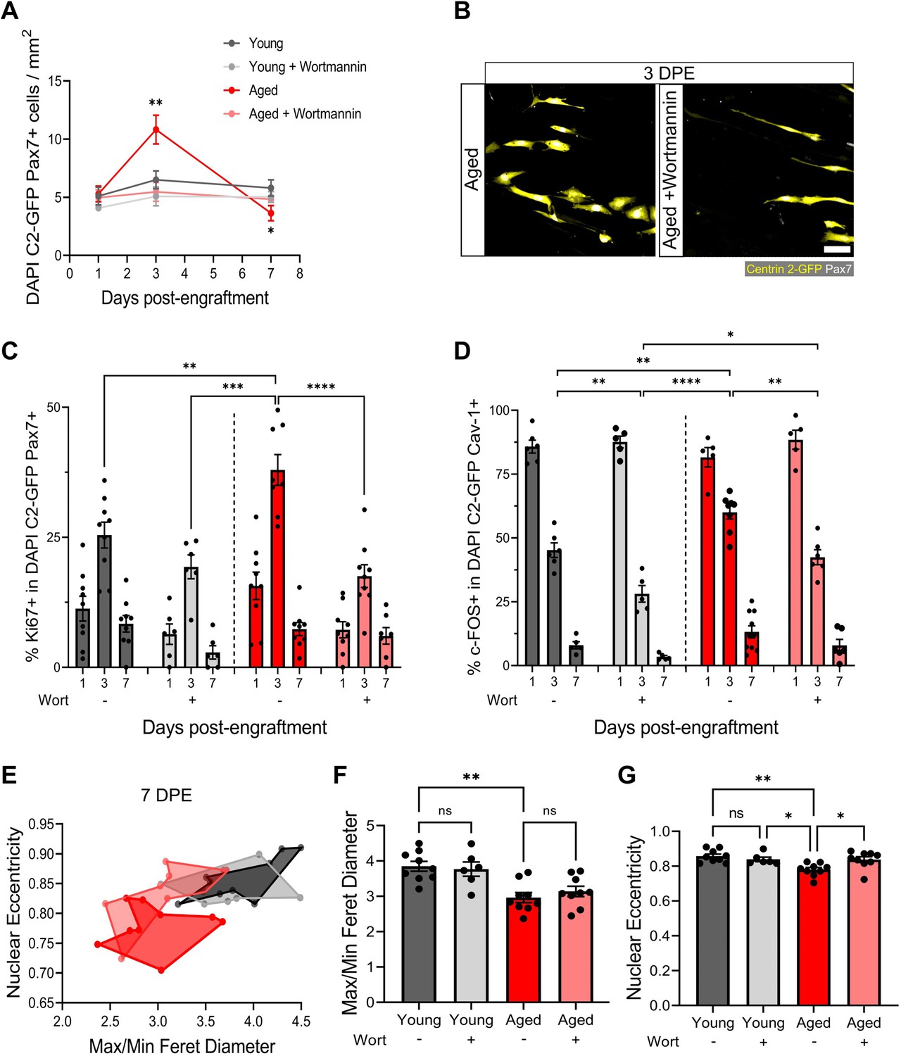
Aberrant pool size maintenance and inactivation in aged muscle stem cells (MuSCs) is rescued by wortmannin.
(A) Quantification of mononuclear DAPI+Centrin 2-GFP (C2-GFP)+Pax7+ cell density per mm2 at 1, 3, and 7 days post-engraftment (DPE) between engrafted young and aged MuSCs ± wortmannin (wort) treatment. n=6–9 across N=2–3 independent biological replicates, graph displays mean ± s.e.m.; one-way ANOVA with Dunnet’s test for each individual timepoint comparing against the young condition, *p=0.0262, **p=0.0065. (B) Representative confocal image of donor cells (Centrin 2-GFP:yellow, Pax7:white) from the aged and aged + wortmannin conditions at 3 DPE. Scale bar, 50 µm. (C) Bar graph showing the percentage of Ki67+ cells in the DAPI+C2-GFP+Pax7+ mononucleated population at 1, 3, and 7 DPE across experimental conditions (young: dark grey; young + wortmannin: light grey; aged: red; aged + wortmannin: light red). n=6–9 across N=2–3 independent biological replicates, graph displays mean ± s.e.m. with individual technical replicates; one-way ANOVA with Tukey’s post-test comparing the conditions against each other at the 3 DPE timepoint, **p=0.0064, ***p=0.0003, ****p˂0.0001 (comparisons not shown are ns). (D) Bar graph showing the percentage of c-FOS+ cells in the DAPI+C2-GFP+Cav-1+ mononucleated population at 1, 3, and 7 DPE across experimental conditions (young: dark grey; young + wortmannin: light grey; aged: red; aged + wortmannin: light red). n=5–10 across N=2–3 independent biological replicates, graph displays mean ± s.e.m. with individual technical replicates; one-way ANOVA with Tukey’s post-test comparing the conditions against each other at the 3 DPE timepoint, *p=0.0169, **p=0.0040, 0.0053, 0.0010, ****p˂0.0001 (comparisons not shown are ns). (E) Dot graph where each dot represents the average max/min Feret diameter ratio and nuclear eccentricity of the Pax7+ donor cells within the technical replicate (tissue) at the 7 DPE timepoint, colour coded according to experimental condition (young: dark grey; young + wortmannin: light grey; aged: red; aged + wortmannin: light red). (F) Bar graph showing the average max/min Feret diameter ratio across experimental conditions, graph displays mean ± s.e.m. with the individual technical replicates from panel E; one-way ANOVA with Tukey’s post-test, **p=0.0010 young vs. aged + wortmannin and young + wortmannin vs. aged are also **p=0.0093, 0.0084, but not shown. All other comparisons are not significant. (G) Bar graph showing the average nuclear eccentricity across experimental conditions, graph displays mean ± s.e.m. with the individual technical replicates from panel (E); one-way ANOVA with Tukey’s post-test, *p=0.0402, 0.0216, **p=0.0015. All other comparisons are not significant. Raw data available in Figure 7—source data 1.
-
Figure 7—source data 1
Raw data for Figure 7.
Data for subpanels separated into tabs.
- https://cdn.elifesciences.org/articles/81738/elife-81738-fig7-data1-v2.xlsx
Figure 7—figure supplement 1
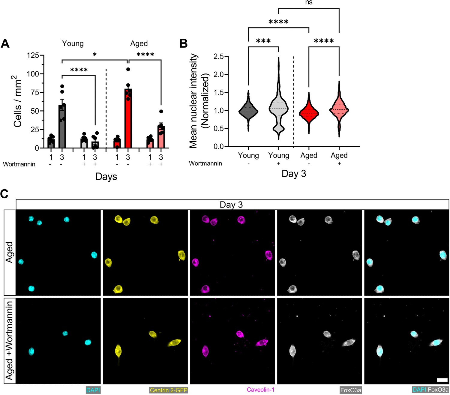
Wortmannin treatment blunts cell proliferation and increases FoxO3a nuclear localization in young and aged muscle stem cells (MuSCs) cultured in vitro.
(A) Bar graph showing the mean number of MuSCs per mm2 of 2D microwells on days 1 and 3 across experimental conditions (young: dark grey; young + wortmannin: light grey; aged: red; aged + wortmannin: light red). n=6 across N=2 independent biological replicates. Graph displays mean ± s.e.m. with the individual technical replicates; one-way ANOVA with Tukey’s post-test comparing each experimental group at the 3 days post-engraftment (DPE) timepoint, *p=0.0353, ****p˂0.0001. (B) Violin plot showing the mean nuclear fluorescent intensity of FoxO3a in MuSCs cultured in two-dimensional (2D) microwells on day 3 across experimental conditions (young: dark grey; young + wortmannin: light grey; aged: red; aged + wortmannin: light red). n=2716, 565, 4437, 1897 across N=2 independent biological replicates. Graph displays mean with first and third quartiles. Data was normalized to the average intensity of the young condition and outliers identified using the ROUT method (with Q=1%) were removed; one-way ANOVA with Šidák’s post-test comparing pre-selected conditions, ****p=0.0002, ****p˂0.0001. Raw data available in Figure 7—figure supplement 1—source data 1.
-
Figure 7—figure supplement 1—source data 1
Raw data for Figure 7—figure supplement 1.
Data for subpanels separated into tabs.
- https://cdn.elifesciences.org/articles/81738/elife-81738-fig7-figsupp1-data1-v2.xlsx
Figure 7—figure supplement 2
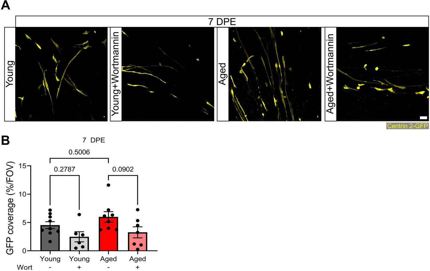
Wortmannin treatment diminishes GFP coverage at 7 days post-engraftment (DPE).
(A) Representative confocal images of the Centrin 2-GFP area coverage (yellow) at 7 DPE from young and aged engrafted muscle stem cells (MuSCs) treated with dimethyl sulfoxide (DMSO) control or wortmannin. Scale bar, 50 µm. (B) Bar graph showing the average GFP coverage (from the Centrin 2-GFP reporter) per field of view at 7 DPE across experimental conditions (young: dark grey; young + wortmannin: light grey; aged: red; aged + wortmannin: light red). n=6–9 across N=2–3 independent biological replicates. Graph displays mean ± s.e.m. with the individual technical replicates; one-way ANOVA with Tukey’s post-test (comparisons not shown are not significant). Raw data available in Figure 7—figure supplement 2—source data 1.
-
Figure 7—figure supplement 2—source data 1
Raw data for Figure 7—figure supplement 2.
Data for subpanels separated into tabs.
- https://cdn.elifesciences.org/articles/81738/elife-81738-fig7-figsupp2-data1-v2.xlsx
Author response image 1

Author response image 2
Tables
Table 1
Cell culture media and solutions.
| Media | Composition |
|---|---|
| FACS Buffer | PBS, 2.5% Goat serum (Gibco, #16210072), 2 mM EDTA (Sigma-Aldrich, #E5134) |
| RBC Lysis Buffer | ddH2O, 0.155 M NH4Cl (Sigma-Aldrich, #A9434), 0.01 M KHCO3 (Sigma-Aldrich, #237205), 0.1 mM EDTA |
| MACS Buffer | PBS, 0.5% Bovine serum albumin (BioShop, #9048-46-8), 2 mM EDTA |
| SAT10 | DMEM/F12 (Gibco, #11320-033), 1% Penicillin-streptomycin (Gibco, #15140-122), 20% Fetal bovine serum (Gibco, 12483-020), 10% Horse serum (Gibco, #16050-122), 1% Glutamax (Gibco, #35050-061), 1% Insulin-transferrin-selenium (Gibco, #41400-045), 1% Non-essential amino acids (Gibco, #11140-050), 1% Sodium pyruvate (Gibco, #11360-070), 50 µM β-mercaptoethanol (Gibco, #21985-023), 5 ng/mL bFGF (ImmunoTools, #11343625) |
| Growth media (GM) | SAT10 – bFGF, 1.5 mg/mL Aminocaproic acid (Sigma-Aldrich, #A2504) |
| Differentiation media (DM) | DMEM (Gibco, #11995-065), 2% Horse serum, 2 mg/mL Aminocarpoic acid, 10 µg/mL Insulin (Sigma, #I6634), 1% Penicillin-streptomycin |
| Blocking Solution | PBS, 10% Goat serum, 0.3% Triton X-100 (BioShop, #TRX777) |
| Physiological Salt Solution (PSS) | 140 mM NaCl (Sigma-Aldrich, #S5886), 5 mM KCl (Sigma-Aldrich, #P3911), 1 mM MgCl2 (Alfa Aesar, #7786-30-3), 10 mM HEPES (BioShop, #7365-45-9), 10 mM Glucose (Sigma-Aldrich, #G8270), 2 mM CaCl2 (Sigma-Aldrich, #C1016), corrected to pH 7.3–7.4 |
| Wash Media | 89% DMEM, 10% Fetal bovine serum, 1% Penicillin-streptomycin |
Table 2
Antibodies.
| Antibody | Host Species | Dilution | Manufacturer |
|---|---|---|---|
| DAPI | – | 1:1000 | Roche, #10236276001 |
| Phalloidin 568 | – | 1:400 | Life Technologies, #A12380 |
| Propidium iodide | – | 1:1000 | Sigma-Aldrich, #P4863 |
| DRAQ5 | – | 1:800 | Cell Signaling Technology, #4084L |
| Anti-sarcomeric α-actinin | Mouse | 1:800 | Sigma-Aldrich, #A7811 |
| Anti-GFP | Chicken | 1:500 | Abcam, #ab13970 |
| Anti-Pax7 | Mouse IgG1 | 1.5:1 | In-house supernatant from hybridoma cell line (DSHB) |
| Anti-caveolin-1 | Rabbit | 1:300 | Abcam, #ab2910 |
| Anti-c-FOS | Mouse IgG1 | 1:250 | Santa-Cruz, #sc-166940 |
| Anti-Ki67 | Rabbit | 1:300 | Abcam, #ab16667 |
| Anti-N-cadherin | Mouse IgG1 | 1:250 | Santa-Cruz, #sc-8424 |
| Anti-MyoD | Mouse IgG2b | 1:300 | Santa-Cruz, #sc-377460 |
| Anti-CalcR | Rabbit | 1:250 | Abcam, #ab11042 |
| Anti-DDX6 | Rabbit | 1:400 | Cederlane Labs, #A300-461A-T |
| Anti-Integrin α-7 | Rabbit | 1:250 | Abcam, #ab203254 |
| Anti-M-cadherin | Mouse IgG1 | 1:250 | Santa-Cruz, #sc-81471 |
| Anti-Laminin α-2 | Rat | 1:400 | Abcam, #ab11576 |
| Anti-FoxO3a | Mouse IgG1 | 1:250 | Santa-Cruz, #sc-48348 |
| Alexa Fluor 488 Anti-mouse IgG (H+L) | Goat | 1:500 | Invitrogen, #A11001 |
| Alexa Fluor 488 Anti-chicken IgGY (H+L) | Goat | 1:500 | Invitrogen, #A11039 |
| Alexa Fluor 546 Anti-mouse IgG (H+L) | Goat | 1:250 | Invitrogen, #A11003 |
| Alexa Fluor 546 Anti-rabbit IgG (H+L) | Goat | 1:250 | Invitrogen, #A11010 |
| Alexa Fluor 546 Anti-rat IgG (H+L) | Goat | 1:400 | Invitrogen, #A11081 |
| Alexa Fluor 546 Anti-mouse IgG2b | Goat | 1:300 | Invitrogen, #A21141 |
| Alexa Fluor 555 picolyl azide | – | 1.2:500 | Invitrogen, #C10638B |
| Alexa Fluor 647 Anti-mouse IgG1 | Goat | 1:250 | Invitrogen, #A21240 |
| Alexa Fluor 647 Anti-rabbit IgG (H+L) | Goat | 1:250 | Life Technologies, #A21245 |
Table 3
Experimental replicate breakdown and statistical analysis.
| Figure | Independent technical and biological replicates (n, N) | Images per technical replicate (tissue) | n to calculate statistics/error bars | Statistical test |
|---|---|---|---|---|
| 1D | SAA coverage Day 2: n=12 across N=4 Day 5: n=12 across N=4 Day 10: n=15 across N=5 Day 14: n=15 across N=5 Day 16: n=12 across N=4 Day 18: n=12 across N=4 Fusion index Day 2: n=9 across N=3 Day 5: n=12 across N=4 Day 10: n=18 across N=6 Day 14: n=15 across N=5 Day 16: n=6 across N=2 Day 18: n=12 across N=4 | SAA coverage: 21 images stitched together Fusion Index: 9 | SAA coverage Day 2: n=12 Day 5: n=12 Day 10: n=15 Day 14: n=15 Day 16: n=12 Day 18: n=12 Fusion index Day 2: n=9 Day 5: n=12 Day 10: n=18 Day 14: n=15 Day 16: n=6 Day 18: n=12 | One-way ANOVA with Tukey’s post-test |
| 1E | Day 2: n=12 across N=4 Day 5: n=12 across N=4 Day 10: n=9 across N=3 Day 14: n=12 across N=4 Day 16: n=12 across N=4 Day 18: n=9 across N=3 | 3 reads | Day 2: n=12 Day 5: n=12 Day 10: n=9 Day 14: n=12 Day 16: n=12 Day 18: n=9 | One-way ANOVA with Tukey’s post-test |
| 2D | 200 MuSCs 1DPE: n=11 across N=4 3DPE: n=12 across N=4 7DPE: n=12 across N=4 500 MuSCs 1DPE: n=8 across N=3 3DPE: n=8 across N=3 7DPE: n=9 across N=3 1500 MuSCs 1DPE: n=7 across N=3 3DPE: n=9 across N=3 7DPE: n=11 across N=4 2500 MuSCs 1DPE: n=9 across N=3 3PE: n=8 across N=3 7DPE: n=9 across N=3 | 25 | 200 MuSCs 1DPE: n=11 3DPE: n=12 7DPE: n=12 500 MuSCs 1DPE: n=8 3DPE: n=8 7DPE: n=9 1500 MuSCs 1DPE: n=7 3DPE: n=9 7DPE: n=11 2500 MuSCs 1DPE: n=9 3PE: n=8 7DPE: n=9 | One-way ANOVA with Dunnet’s test for each individual timepoint comparing against the 500 MuSC condition |
| 3B | 1DPE: n=9 across N=3 3DPE: n=9 across N=3 7DPE: n=9 across N=3 | 25 | 1DPE: n=9 3DPE: n=9 7DPE: n=9 | One-way ANOVA with Tukey's post-test comparing the FOS- proportions of each timepoint |
| 3C | 1DPE: n=10 across N=3 3DPE: n=11 across N=4 7DPE: n=11 across N=4 | 25 | 1DPE: n=10 3DPE: n=11 7DPE: n=11 | One-way ANOVA with Tukey’s post-test comparing the Ki67- proportions of each timepoint |
| 3E | n=15 across N=5 | 25 | n=15 | – |
| 3G | PSS n=16 across N=5 2.4% BaCl n=18 across N=6 | 25 | PSS n=16 2.4% BaCl n=18 | Unpaired t-test of the Ki67- proportions of both conditions |
| 4B | 1DPE: n=9 across N=3 3DPE: n=10 across N=3 7DPE: n=9 across N=3 | 25 | 1DPE: n=9 3DPE: n=10 7DPE: n=9 | – |
| 4C | 1DPE: n=9 across N=3 3DPE: n=9 across N=3 7DPE: n=9 across N=3 | 25 | 1DPE: n=9 3DPE: n=9 7DPE: n=9 | – |
| 4D | 1DPE: n=6 across N=2 3DPE: n=6 across N=2 7DPE: n=6 across N=2 | 25 | 1DPE: n=6 3DPE: n=6 7DPE: n=6 | – |
| 4E | 1DPE: n=6 across N=2 3DPE: n=6 across N=2 7DPE: n=6 across N=2 | 25 | 1DPE: n=6 3DPE: n=6 7DPE: n=6 | – |
| 4F | 1DPE: n=15 across N=4 3DPE: n=14 across N=4 7DPE: n=13 across N=4 | 25 | 1DPE: n=15 3DPE: n=14 7DPE: n=13 | – |
| 5C | 1DPE: n=916 across N=4 3DPE: n=980 across N=4 7DPE: n=737 across N=3 | 25 | – | – |
| 5E | 1DPE: n=639 across N=3 3DPE: n=770 across N=3 7DPE: n=676 across N=3 | 25 | 1DPE: n=639 3DPE: n=770 7DPE: n=676 | One-way ANOVA with Tukey’s post-test |
| 5F | n=676 across N=3 | 25 | Bin 2=147 Bin 3=135 Bin 4=89 Bin 5=69 Bin 6=66 Bin 7=48 Bin 8=44 Bin 9=30 Bin 9+=48 | One-way ANOVA with test for linear trend |
| 6C | n=8 across N=3 | 25 | – | – |
| 6D | n=8 across N=3 | 45 | – | – |
| 7A | Young 1DPE: n=9 across N=3 3DPE: n=9 across N=3 7DPE: n=9 across N=3 Young + wortmannin 1DPE: n=6 across N=2 3DPE: n=6 across N=2 7DPE: n=6 across N=2 Aged 1DPE: n=9 across N=3 3DPE: n=8 across N=3 7DPE: n=9 across N=3 Aged + wortmannin 1DPE: n=9 across N=3 3DPE: n=9 across N=3 7DPE: n=7 across N=3 | 25 | Young 1DPE: n=9 3DPE: n=9 7DPE: n=9 Young + wortmannin 1DPE: n=6 3DPE: n=6 7DPE: n=6 Aged 1DPE: n=9 3DPE: n=8 7DPE: n=9 Aged + wortmannin 1DPE: n=9 3DPE: n=9 7DPE: n=7 | One-way ANOVA with Dunnet’s test for each individual timepoint comparing against the Young condition |
| 7C | Young 1DPE: n=9 across N=3 3DPE: n=9 across N=3 7DPE: n=9 across N=3 Young + wortmannin 1DPE: n=6 across N=2 3DPE: n=6 across N=2 7DPE: n=6 across N=2 Aged 1DPE: n=9 across N=3 3DPE: n=8 across N=3 7DPE: n=9 across N=3 Aged + wortmannin 1DPE: n=9 across N=3 3DPE: n=9 across N=3 7DPE: n=7 across N=3 | 25 | Young 1DPE: n=9 3DPE: n=9 7DPE: n=9 Young + wortmannin 1DPE: n=6 3DPE: n=6 7DPE: n=6 Aged 1DPE: n=9 3DPE: n=8 7DPE: n=9 Aged + wortmannin 1DPE: n=9 3DPE: n=9 7DPE: n=7 | One-way ANOVA with Tukey’s post-test comparing the conditions against each other at the 3 DPE timepoint |
| 7D | Young 1DPE: n=6 across N=2 3DPE: n=6 across N=2 7DPE: n=5 across N=2 Young + wortmannin 1DPE: n=5 across N=2 3DPE: n=5 across N=2 7DPE: n=5 across N=2 Aged 1DPE: n=5 across N=2 3DPE: n=8 across N=3 7DPE: n=10 across N=3 Aged + wortmannin 1DPE: n=5 across N=2 3DPE: n=6 across N=2 7DPE: n=6 across N=2 | 25 | Young 1DPE: n=6 3DPE: n=6 7DPE: n=5 Young + wortmannin 1DPE: n=5 3DPE: n=5 7DPE: n=5 Aged 1DPE: n=5 3DPE: n=8 7DPE: n=10 Aged + wortmannin 1DPE: n=5 3DPE: n=6 7DPE: n=6 | One-way ANOVA with Tukey’s post-test comparing the conditions against each other at the 3 DPE timepoint |
| 7E | Young n=9 across N=3 Young + wortmannin n=6 across N=2 Aged n=9 across N=3 Aged + wortmannin n=9 across N=3 | 25 | – | – |
| 7F | Young n=9 across N=3 Young + wortmannin n=6 across N=2 Aged n=9 across N=3 Aged + wortmannin n=9 across N=3 | 25 | Young n=9 Young + wortmannin n=6 Aged n=9 Aged + wortmannin n=9 | One-way ANOVA with Tukey’s post-test |
| 7G | Young n=9 across N=3 Young + wortmannin n=6 across N=2 Aged n=9 across N=3 Aged + wortmannin n=9 across N=3 | 25 | Young n=9 Young + wortmannin n=6 Aged n=9 Aged + wortmannin n=9 | One-way ANOVA with Tukey’s post-test |
| F1-S1B | 10,000 n=12 across N=4 25,000 n=12 across N=4 50,000 n=12 across N=4 | 21 images stitched together | 10,000 n=12 25,000 n=12 50,000 n=12 | One-way ANOVA with Tukey’s post-test |
| F1-S2C | 3D 1DPE: n=6 across N=3 3DPE: n=9 across N=3 7DPE: n=9 across N=3 2 D 1DPE: n=9 across N=3 3DPE: n=9 across N=3 7DPE: n=9 across N=3 | 21 images stitched together | 3D 1DPE: n=6 3DPE: n=9 7DPE: n=9 2D 1DPE: n=9 3DPE: n=9 7DPE: n=9 | One-way ANOVA with Tukey’s post-test |
| F1-S2D | 3D 1DPE: n=6 across N=3 3DPE: n=9 across N=3 7DPE: n=9 across N=3 2 D 1DPE: n=9 across N=3 3DPE: n=9 across N=3 7DPE: n=9 across N=3 | 25 | 3D 1DPE: n=6 3DPE: n=9 7DPE: n=9 2D 1DPE: n=9 3DPE: n=9 7DPE: n=9 | One-way ANOVA with Tukey’s post-test |
| F1-S2E | 3D 1DPE: n=6 across N=3 3DPE: n=9 across N=3 7DPE: n=9 across N=3 2 D 1DPE: n=9 across N=3 3DPE: n=9 across N=3 7DPE: n=9 across N=3 | 2 | 3D 1DPE: n=6 3DPE: n=9 7DPE: n=9 2D 1DPE: n=9 3DPE: n=9 7DPE: n=9 | One-way ANOVA with Tukey’s post-test |
| F1-S2F | 3D 1DPE: n=6 across N=3 3DPE: n=9 across N=3 7DPE: n=9 across N=3 2 D 1DPE: n=9 across N=3 3DPE: n=9 across N=3 7DPE: n=9 across N=3 | 2 | 3D 1DPE: n=6 3DPE: n=9 7DPE: n=9 2D 1DPE: n=9 3DPE: n=9 7DPE: n=9 | One-way ANOVA with Tukey’s post-test |
| F1-S2G | 3D 1DPE: n=6 across N=3 3DPE: n=9 across N=3 7DPE: n=9 across N=3 2 D 1DPE: n=9 across N=3 3DPE: n=9 across N=3 7DPE: n=9 across N=3 | 2 | 3D 1DPE: n=6 3DPE: n=9 7DPE: n=9 2D 1DPE: n=9 3DPE: n=9 7DPE: n=9 | One-way ANOVA with Tukey’s post-test |
| F2-S1C | n=11 across N=4 | 25 | n=11 | – |
| F3-S1B | 1DPE: n=8 across N=3 3DPE: n=7 across N=3 7DPE: n=15 across N=5 | 25 | 1DPE: n=8 3DPE: n=7 7DPE: n=15 | One-way ANOVA with Tukey’s post-test |
| F3-S2A | BI n=8 across N=3 PSS n=7 across N=3 2.4% BaCl n=9 across N=3 | 21 images stitched together | BI n=8 PSS n=7 2.4% BaCl n=9 | One-way ANOVA with Tukey’s post-test |
| F3-S2B | BI n=7 across N=3 PSS n=9 across N=3 2.4% BaCl n=9 across N=3 | 25 | BI n=7 PSS n=9 2.4% BaCl n=9 | One-way ANOVA with Tukey’s post-test |
| F3-S3C | 200 MuSCs n=11 across N=4 500 MuSCs n=15 across N=5 1500 MuSCs n=16 across N=5 2500 MuSCs n=13 across N=4 | 25 | 200 MuSCs n=11 500 MuSCs n=15 1500 MuSCs n=16 2500 MuSCs n=13 | One-way ANOVA with Tukey’s post-test |
| F3-S3D | 200 MuSCs n=12 across N=4 500 MuSCs n=9 across N=3 1500 MuSCs n=12 across N=4 2500 MuSCs n=9 across N=4 | 25 | 200 MuSCs n=12 500 MuSCs n=9 1500 MuSCs n=12 2500 MuSCs n=9 | One-way ANOVA with Tukey’s post-test |
| F4-S1B | Day 5 n=15 across N=5 Day 0 n=11 across N=4 | 25 | Day 5 n=15 5 Day 0 n=11 | Unpaired t-test |
| F5-S1B | 2D n=9 across N=3 2D+myotubes n=8 across N=3 3D+myotubes n=14 across n=3 | 25 | 2D n=9 2D+myotubes n=8 3D+myotubes n=14 | One-way ANOVA with Tukey’s post-test |
| F5-S1C | 2D n=9 across N=3 2D+myotubes n=8 across N=3 3D+myotubes n=14 across n=3 | 25 | 2D n=9 2D+myotubes n=8 3D+myotubes n=14 | One-way ANOVA with Tukey’s post-test |
| F5-S2C | 1DPE: n=35 across N=3 3DPE: n=45 across N=3 7DPE: n=45 across N=3 | Every 5 images is from 1 tissue | n=125 | Simple linear regression |
| F5-S3A | 1DPE: n=916 across N=4 3DPE: n=980 across N=4 7DPE: n=737 across N=3 | 25 | 1DPE: n=916 3DPE: n=980 7DPE: n=737 | – |
| F5-S3C | Pax7+/MyoD- 3DPE: n=12 across N=4 7DPE: n=11 across N=3 Pax7+/MyoD+ 3DPE: n=11 across N=4 7DPE: n=10 across N=3 | 25 | Pax7+/MyoD- 3DPE: n=12 7DPE: n=11 Pax7+/MyoD+ 3DPE: n=11 7DPE: n=10 | Unpaired t-tests |
| F5-S4B | Control 1DPE: n=7 across N=3 3DPE: n=8 across N=3 7DPE: n=9 across N=3 Y-27632 1DPE: n=9 across N=3 3DPE: n=9 across N=3 7DPE: n=9 across N=3 | 25 | Control 1DPE: n=7 3DPE: n=8 7DPE: n=9 Y-27632 1DPE: n=9 3DPE: n=9 7DPE: n=9 | Unpaired t-tests for each individual timepoint |
| F5-S4C | Control 1DPE: n=6 across N=2 3DPE: n=6 across N=2 7DPE: n=6 across N=2 Y-27632 1DPE: n=6 across N=2 3DPE: n=6 across N=2 7DPE: n=6 across N=2 | 25 | Control 1DPE: n=6 3DPE: n=6 7DPE: n=6 Y-27632 1DPE: n=6 3DPE: n=6 7DPE: n=6 | Unpaired t-tests for each individual timepoint |
| F5-S4D | Control 1DPE: n=7 across N=3 3DPE: n=8 across N=3 7DPE: n=9 across N=3 Y-27632 1DPE: n=9 across N=3 3DPE: n=9 across N=3 7DPE: n=9 across N=3 | 25 | Control 1DPE: n=7 3DPE: n=8 7DPE: n=9 Y-27632 1DPE: n=9 3DPE: n=9 7DPE: n=9 | Unpaired t-tests for each individual timepoint |
| F5-S5A | Control 1DPE: n=666 across N=3 3DPE: n=994 across N=3 7DPE: n=783 across N=3 Y-27632 1DPE: n=1,255 across N=3 3DPE: n=1,158 across N=3 7DPE: n=598 across N=3 | 25 | Control 1DPE: n=666 3DPE: n=994 7DPE: n=783 Y-27632 1DPE: n=1255 3DPE: n=1158 7DPE: n=598 | – |
| F5-S5B | Pax7+/MyoD- and Pax7+/MyoD+(Control 1DPE: n=7 across N=3 3DPE: n=8 across N=3 7DPE: n=9 across N=3 Y-27632 1DPE: n=9 across N=3 3DPE: n=9 across N=3 7DPE: n=9 across N=3) | 25 | Pax7+/MyoD- and Pax7+/MyoD+ (Control 1DPE: n=7 3DPE: n=8 7DPE: n=9 Y-27632 1DPE: n=9 3DPE: n=9 7DPE: n=9) | One-way ANOVA with Tukey’s post-test within each individual timepoints |
| F5-S5C | Pax7+/MyoD- and Pax7+/MyoD+(Control 1DPE: n=7 across N=3 3DPE: n=8 across N=3 7DPE: n=9 across N=3 Y-27632 1DPE: n=9 across N=3 3DPE: n=9 across N=3 7DPE: n=9 across N=3) | 25 | Pax7+/MyoD- and Pax7+/MyoD+ (Control 1DPE: n=7 3DPE: n=8 7DPE: n=9 Y-27632 1DPE: n=9 3DPE: n=9 7DPE: n=9) | One-way ANOVA with Tukey’s post-test within each individual timepoints |
| F5-S5E | Pax7+/MyoD- and Pax7+/MyoD+(Control 1DPE: n=7 across N=3 3DPE: n=8 across N=3 7DPE: n=9 across N=3 Y-27632 1DPE: n=9 across N=3 3DPE: n=9 across N=3 7DPE: n=9 across N=3) | 25 | Control 1DPE: n=7 3DPE: n=8 7DPE: n=9 Y-27632 1DPE: n=9 3DPE: n=9 7DPE: n=9 | One-way ANOVA with Tukey’s post-test within each individual timepoints |
| F5-S5F | Pax7+/MyoD- and Pax7+/MyoD+(Control 1DPE: n=7 across N=3 3DPE: n=8 across N=3 7DPE: n=9 across N=3 Y-27632 1DPE: n=9 across N=3 3DPE: n=9 across N=3 7DPE: n=9 across N=3) | 25 | Pax7+/MyoD- and Pax7+/MyoD+ (Control 1DPE: n=7 3DPE: n=8 7DPE: n=9 Y-27632 1DPE: n=9 3DPE: n=9 7DPE: n=9) | One-way ANOVA with Tukey’s post-test within each individual timepoints |
| F7-S1A | Young Day 1: n=6 across N=2 Day 3: n=6 across N=2 Young + wortmannin Day 1: n=6 across N=2 Day 3: n=6 across N=2 Aged Day 1: n=6 across N=2 Day 3: n=6 across N=2 Aged + wortmannin Day 1: n=6 across N=2 Day 3: n=6 across N=2 | 104 | Young Day 1: n=6 Day 3: n=6 Young + wortmannin Day 1: n=6 Day 3: n=6 Aged Day 1: n=6 Day 3: n=6 Aged + wortmannin Day 1: n=6 Day 3: n=6 | One-way ANOVA with Tukey’s post-test comparing each experimental group at the 3 DPE timepoint |
| F7-S1B | Young n=2716 across N=2 Young + wortmannin n=565 across N=2 Aged n=4437 across N=2 Aged + wortmannin n=1897 across N=2 | 104 | Young n=2716 Young + wortmannin n=565 Aged n=4437 Aged + wortmannin n=1897 | Outliers removed with the ROUT method (with Q=1%) and one-way ANOVA performed with Šidák’s post-test comparing pre-selected conditions |
| F7-S2B | Young n=9 across N=3 Young + wortmannin n=6 across N=2 Aged n=8 across N=3 Aged + ortmannin n=7 across N=3 | 25 | Young n=9 Young + wortmannin n=6 Aged n=8 Aged + wortmannin n=7 | One-way ANOVA with Tukey’s post-test |
Additional files
Download links
A two-part list of links to download the article, or parts of the article, in various formats.
Downloads (link to download the article as PDF)
Open citations (links to open the citations from this article in various online reference manager services)
Cite this article (links to download the citations from this article in formats compatible with various reference manager tools)
The mini-IDLE 3D biomimetic culture assay enables interrogation of mechanisms governing muscle stem cell quiescence and niche repopulation
eLife 11:e81738.
https://doi.org/10.7554/eLife.81738


