Biological condensates form percolated networks with molecular motion properties distinctly different from dilute solutions
- Division of Life Science, Hong Kong University of Science and Technology, ClearWater Bay, Kowloon, China
- Department of Biochemistry, University of Toronto, Canada
- Department of Physics, Hong Kong University of Science and Technology, Clear Water Bay, Kowloon, China
- Department of Chemical and Biological Engineering, Hong Kong University of Science and Technology, Clear Water Bay, Kowloon, China
- Greater Bay Biomedical Innocenter, Shenzhen Bay Laboratory, China
- School of Life Sciences, Southern University of Science and Technology, China
Figures
Figure 1 with 1 supplement
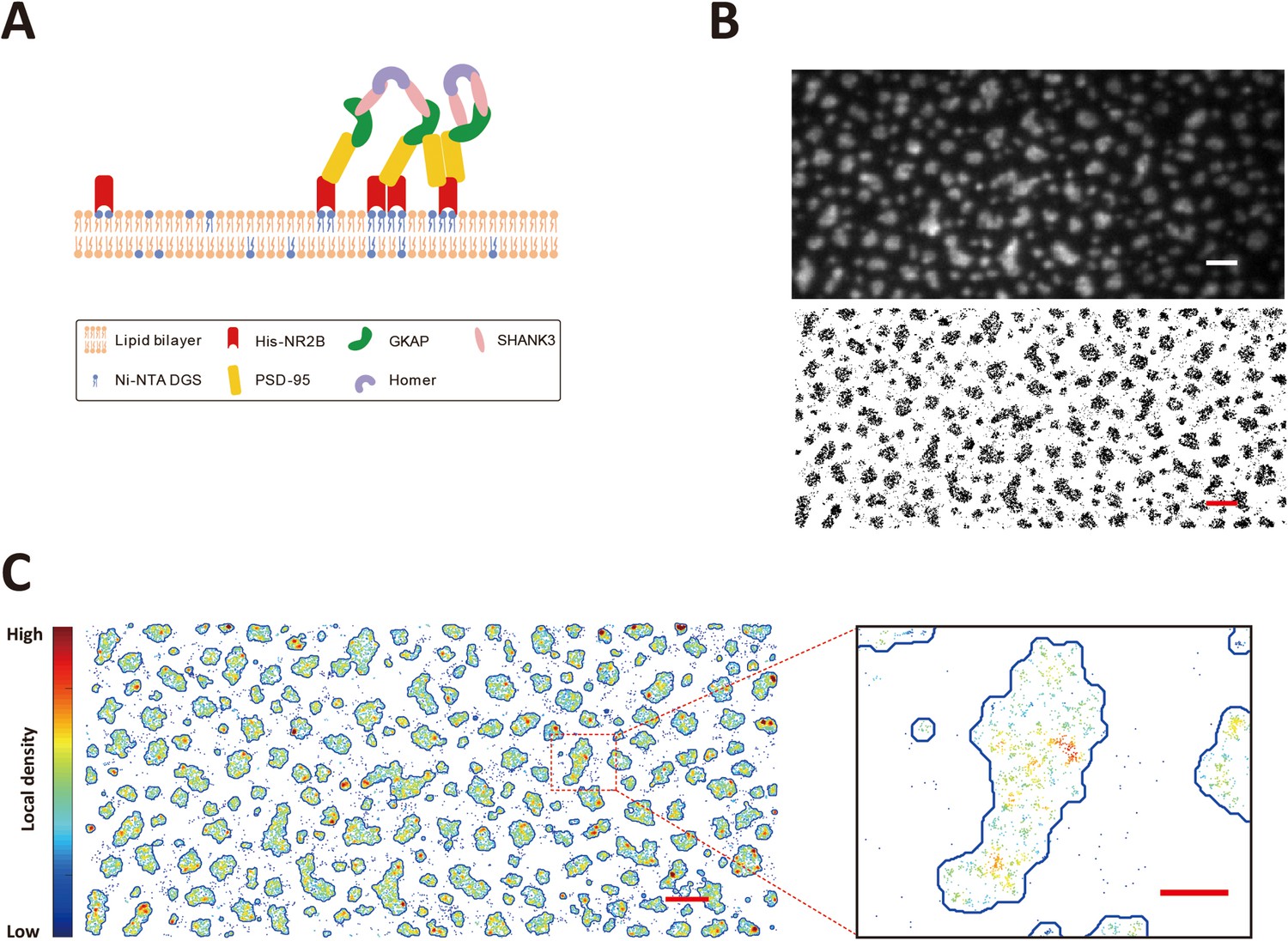
Single-molecule imaging of phase separation on supported lipid bilayers.
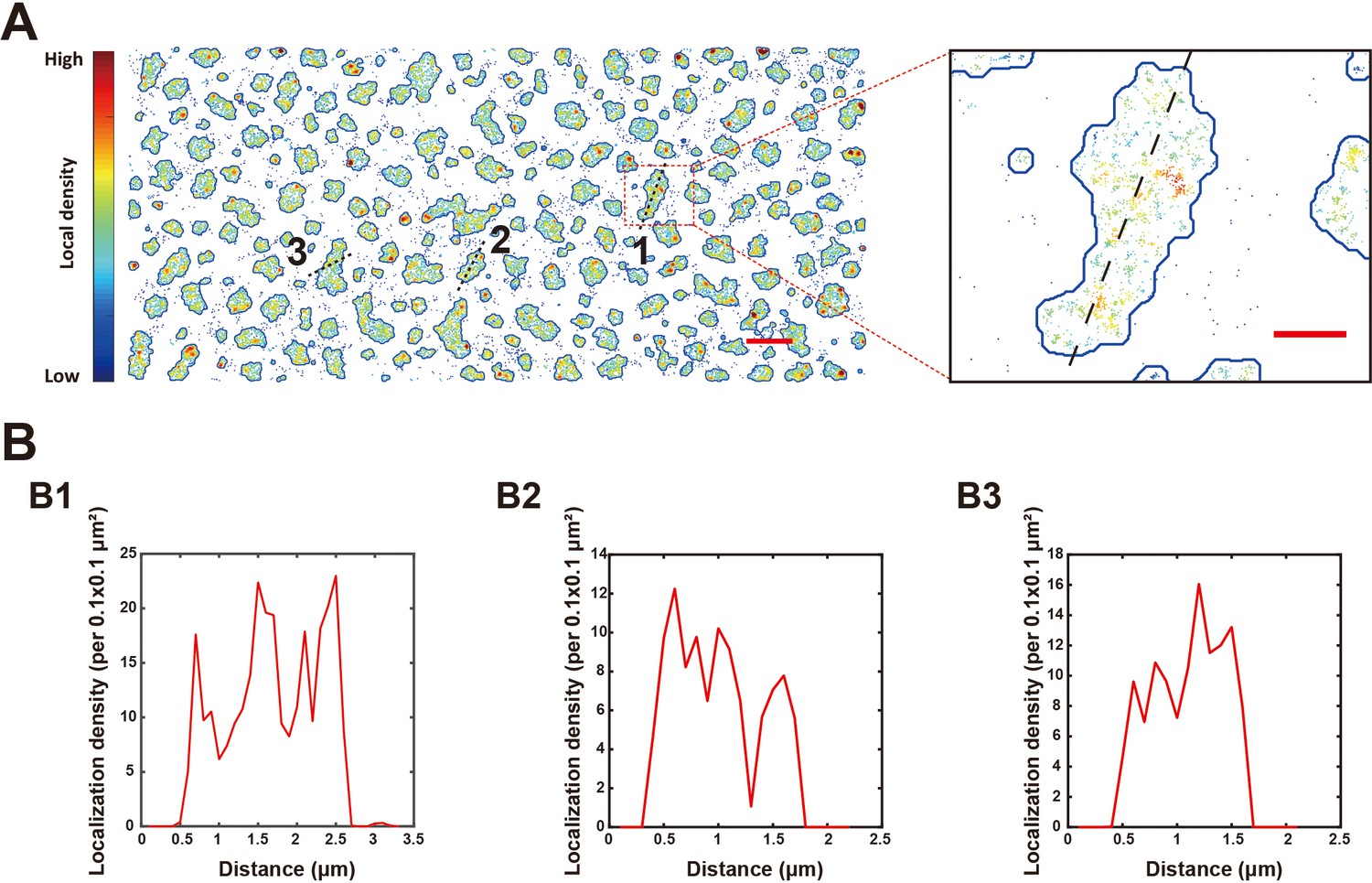
(A) Schematic diagram showing phase separation of postsynaptic density (PSD) protein assembly on supported lipid bilayers (SLBs) (Zeng et al., 2018). (B) Upper panel: a TIRF image of Alexa 647 labeled His8-NR2B tetramer clustered within the PSD condensate on SLB. Lower panel: stacking of 4000 frames of dSTORM images of Alexa 647 labeled His8-NR2B within the same PSD condensates as shown in the TIRF image above. Black dots represent localizations recognized during the imaging. Scale bar: 2 μm. (C) Phase boundary of the PSD condensates determined by localization densities. The boundaries are shown by blue lines. Localizations are color-coded according to their local densities from low (blue) to high (red). A zoom-in view of a typical condensed patch on SLB showing heterogeneous distributions and nano-cluster-like structures of molecules within the condensed phase. Scale bar of the original image: 2 μm, scale bar for the zoom-in view: 500 nm.
Figure 1—figure supplement 1
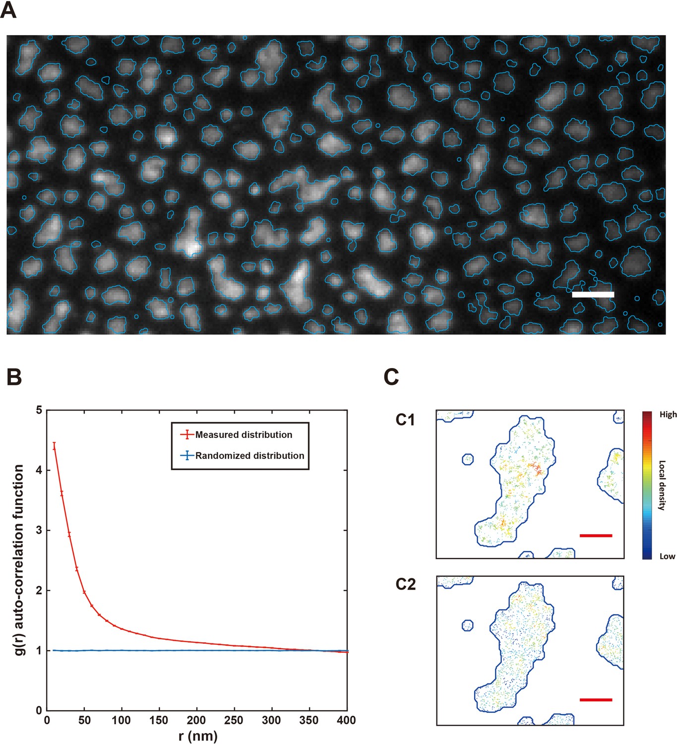
Determination of boundaries of the condensed phase throughout the imaging process and heterogeneous distribution of molecules in the condensed phase.
(A) Wide-field image merged with phase boundaries that were reconstructed from supper-resolution images (blue curves) showing no obvious phase boundary changes during the time duration of the imaging process. Scale bar: 2 μm.(B) Autocorrelation functions of measured NR2B distribution in condensed phase regions (red curve) and a simulated randomized distribution in the same condensed phase regions (blue curve).(C) (C1) A zoom-in view of an example of experimentally measured condensed-phase molecular distribution on supported lipid bilayer (SLB), showing heterogeneous distributions and nano-cluster-like structures of molecules within the condensed phase. (C2) Corresponding view of simulated randomized molecular distribution in the same set of condensed-phase regions with the same total number of molecules as in (C1). Scale bar for the zoom-in view: 500 nm.
Figure 2 with 4 supplements
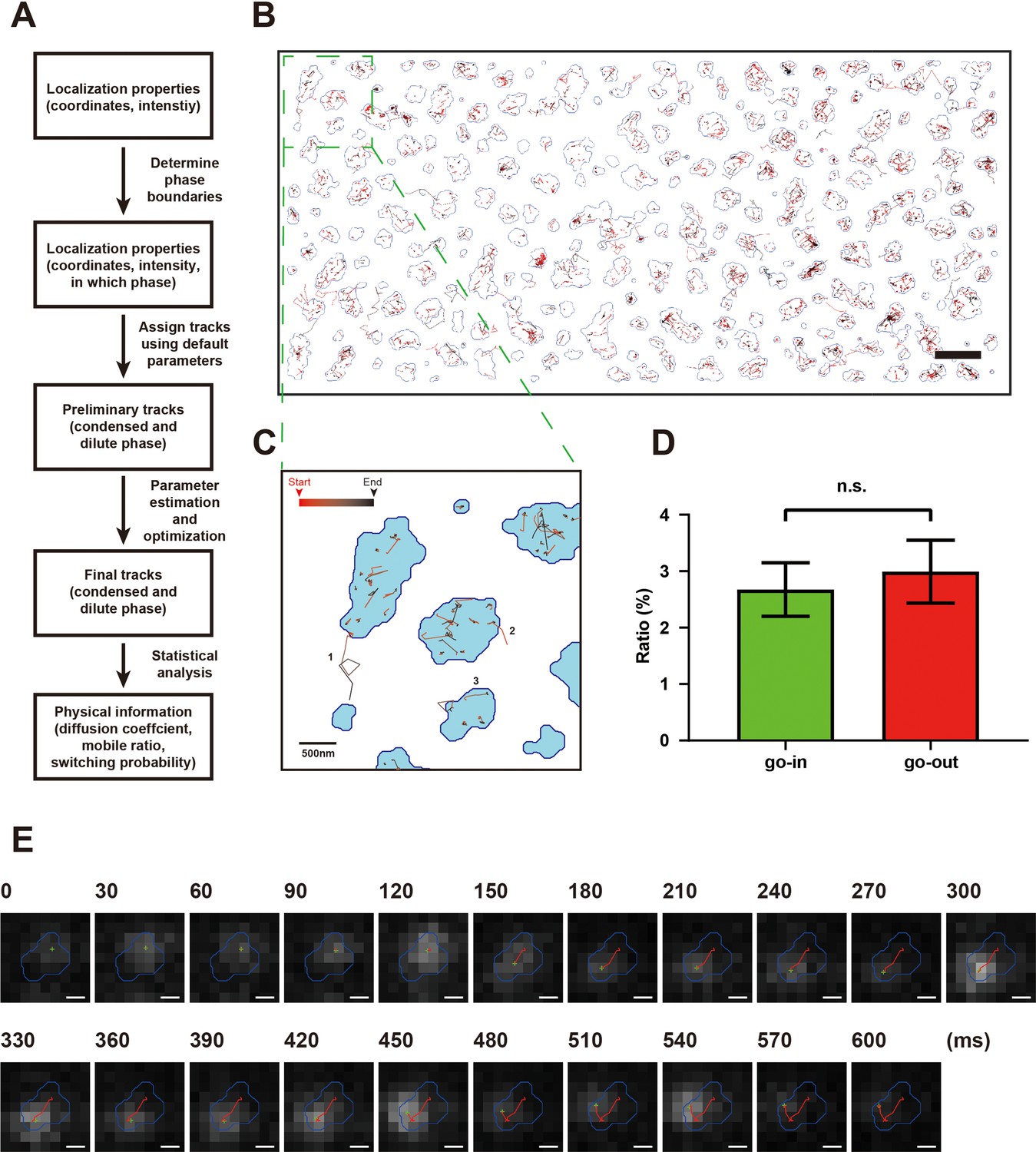
Development of an adaptive single-molecule tracking algorithm for imaging single molecules in the condensed and dilute phases simultaneously.
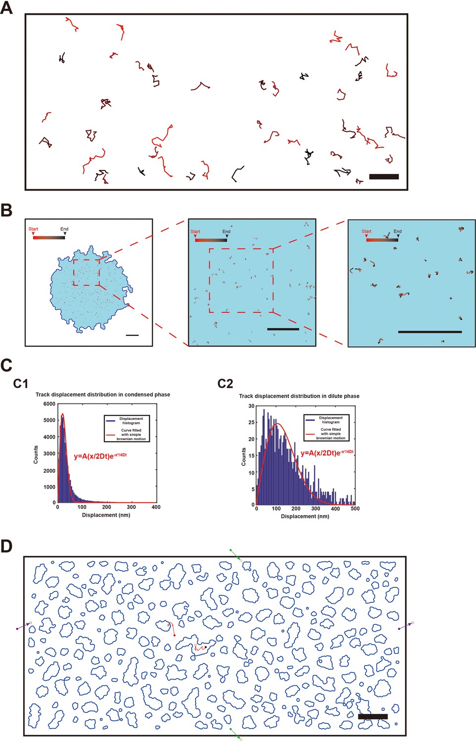
(A) Flowchart of the adaptive single-molecule tracking algorithm. (B) Assignments of motion tracks of NR2B in both condensed and dilute phases in the postsynaptic density (PSD) condensates formed on supported lipid bilayer (SLB). Each track is color-coded from red to black from the beginning to the end of the track. The boundaries of the condensates are marked by blue lines. Scale bar: 2 μm. (C) Representative tracks showing typical NR2B motions. Examples include trajectories involving mobile and/or confined states as well as exchange events of molecules crossing between condensed and dilute phases (tracks 1 and 2) and a trajectory that passes through both the transiently confined and the mobile (more freely diffusing) states in the condensed phase (track 3). (D) Percentages of NR2B molecules exchange from the dilute phase into the condensed phase (‘go-in’) and vice versa (‘go-out’) were counted in four sessions of dSTORM imaging experiments. No significant difference between go-in ratio and go-out ratio was detected. p=0.378 using paired t-test and defined as not significant (n.s.). (E) Raw image data superimposed with phase boundary (blue line), molecule localization (green cross), and track steps (red line) show a typical trajectory of an NR2B molecule undergoing multiple motion switches between confined and mobile states in the condensed phase. Scale bar: 200 nm.
Figure 2—figure supplement 1
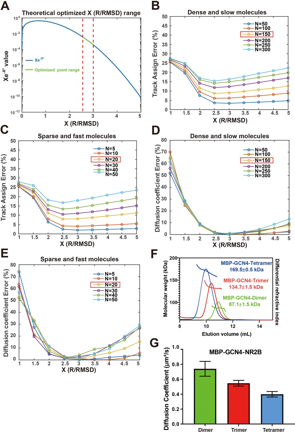
Evaluation of the adaptive single-molecule tracking algorithm by simulation and by experiments.
(A) Determination of the optimized search range. Blue line shows the curve for the left-hand side of the equation , and green line shows the range for the right-hand side of the same equation in typical physical scenarios of phase separation (see ‘Materials and methods’). The red dashed lines delimit the variation of optimized search range in different physical scenarios. (B, C) Simulated track assignment errors of molecules in homogeneous condensed phase with slow diffusion (D ~ 0.1 μm2/s, panel B) or in dilute phase with fast diffusion (D ~ 1.0 μm2/s, panel C) in systems with different molecular densities (N) and maximum step limit/root mean square displacement (RMSD) (R/RMSD) ratios. The experimental molecular density in condensed and dilute phases is around 150/ (15 × 30 μm2) and 20/ (15 × 30 μm2). The red box highlights the situation matching our experimental data for the postsynaptic density (PSD) system. (D, E) Simulated diffusion coefficient errors of molecules in homogeneous condensed phase with slow diffusion (D ~ 0.1 μm2/s, panel D) or in dilute phase with fast diffusion (D ~ 1.0 μm2/s, panel E) in systems with different molecular densities and R/RMSD values. The red box highlights the situation matching our experimental data. (F) Fast protein liquid chromatography (FPLC)-coupled with static light scattering analysis showing the column behavior and measured molecular weight of the purified MBP-His6-GCN4-Dimer, Trimer, and Tetramer. (G) Diffusion coefficient of homogeneous solutions of MBP-His6-GCN4-Dimer, Trimer, and Tetramer derived by our adaptive single-molecule tracking algorithm. The diffusion coefficients were derived by fitting mean square displacement (MSD) as a function of time and shown as mean ± SD for nine independent samples for each protein.
Figure 2—figure supplement 2
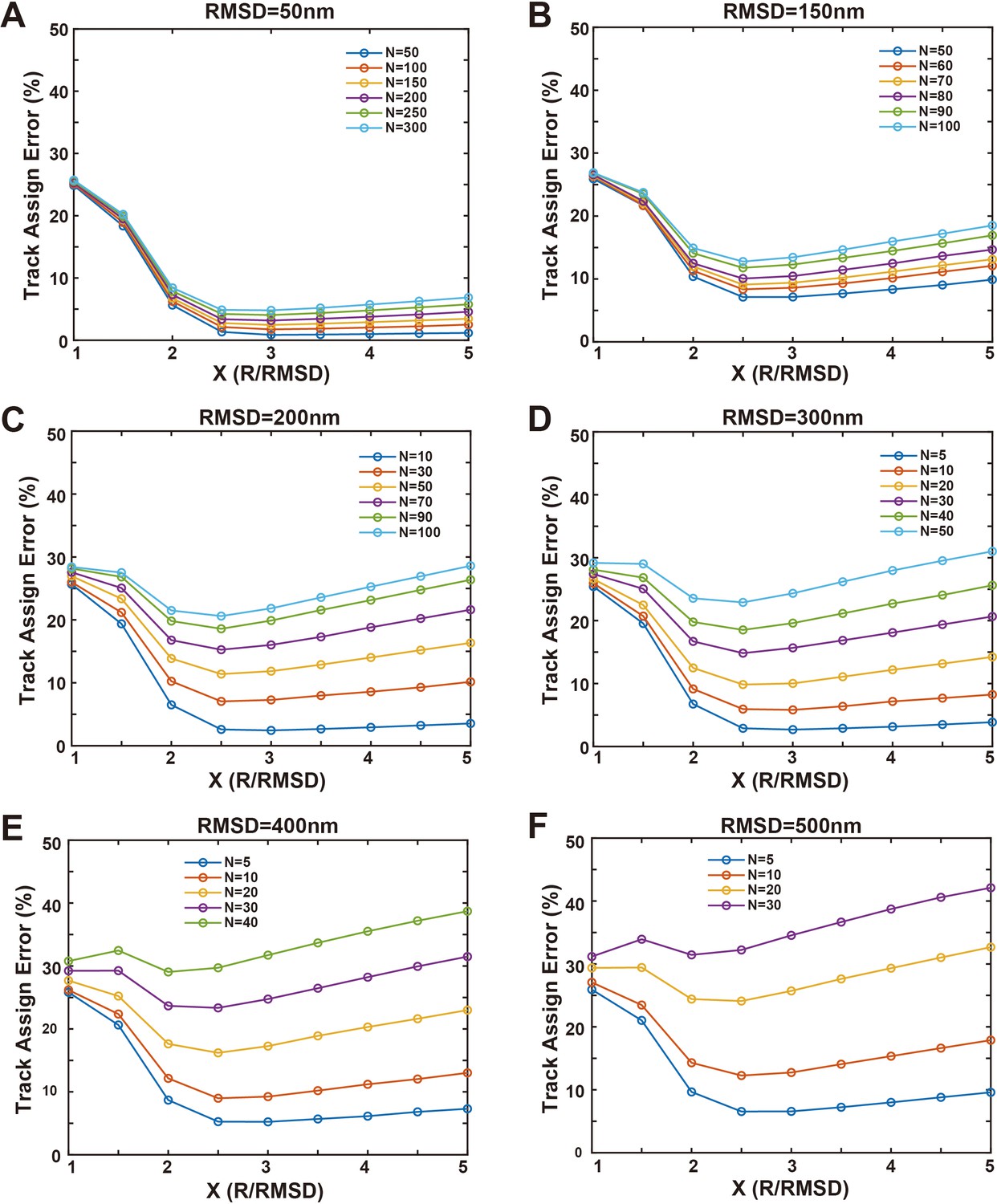
Simulations of track assignment errors of phase separations with molecules in the condensed phase undergoing homogeneous free diffusions.
Simulated track assignment errors vs. maximum step limit/root mean square displacement (RMSD) ratios under different phase separation conditions. Different colors were used to distinguish different average molecule density (N) in every frame. Each panel used different RMSD in consecutive frames: (A) RMSD = 50 nm, (B) RMSD = 150 nm, (C) RMSD = 200 nm, (D) RMSD = 300 nm, (E) RMSD = 400 nm, and (F) RMSD = 500 nm.
Figure 2—figure supplement 3
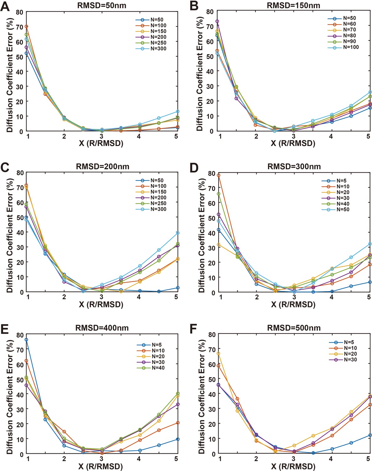
Simulations of diffusion coefficient errors of phase separations with molecules in the condensed phase undergoing homogeneous free diffusions.
Figure 2—figure supplement 4
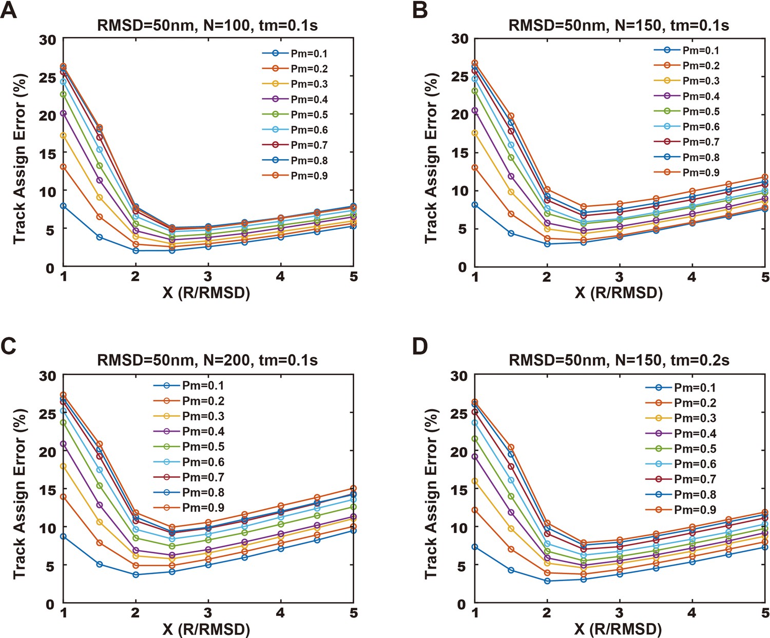
Simulations of track assignment errors of phase separations with molecules in the condensed phase containing both confined and mobile states.
Simulated results of track assignment errors vs. maximum step limit/root mean square displacement (RMSD) ratios under different conditions. Different line colors were used to distinguish different mobile fractions (Pm). RMSD = 100 nm for all panels, but molecular density (N) and dwell time (tm) are different for each condition. (A) N = 100, tm = 0.1 s, (B) N = 150, tm = 0.1 s, (C) N = 200, tm = 0.1 s, and (D) N = 150, tm = 0.2 s.
Figure 3 with 3 supplements
Dynamic parameters and a diffusion model for an equilibrium state phase separation system.
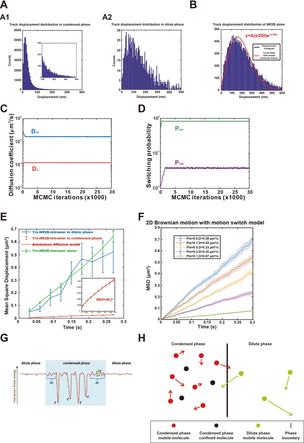
(A) Displacement distribution of tracks in the (A1) condensed and (A2) dilute phases. Zoom-in view in (A1) shows detailed distribution of the distribution tail. Bin size of histogram is 5 nm. (B) Displacement distribution of tracks of NR2B alone tethered to supported lipid bilayer (SLB). Red curve is the fit with a simple 2D Brownian motion distribution obtained by nonlinear least-squares method using MATLAB, here the fitted diffusion coefficient D = 0.46 ± 0.02 μm2/s, square of Pearson correlation coefficient r2 = 0.91, root mean square deviation (RMSE) = 42.5. Bin size of histogram is 5 nm. (C, D) Optimization of the dynamic parameters of NR2B in the postsynaptic density (PSD) condensates formed on SLBs with Hidden Markov Model assuming that NR2B is conforming to a two-state motion model in the condensed phase visiting both a transient confined state and a mobile state. The parameters of interest are diffusion coefficient of the confined state in the condensed phase (Dc) and diffusion coefficient of the mobile state (Dm) in the condensed phase, switching probability from the confined state to the mobile state (Pcm) and the reversed switching probability (Pmc). (E) Determination of the diffusion coefficients of NR2B in dilute phase (blue) by fitting the mean square displacements (MSDs) against time using linear regression. In view of the MSD’s appreciable nonlinear time dependence, motion of NR2B in the condensed phase (red) is fitted by a subdiffusive model, viz., MSD = 4Dαtα. The figure also includes data and linear fit for the control case of NR2B alone tethered to SLB (green). The inset shows a y-axis zoom-in view of NR2B dynamic behavior in the condensed phase to highlight its subdiffusive nature. The number of trajectories used in the fittings was 2443 for the condensed phase, 13 for the dilute phase, and 248 for NR2B alone on SLB. Note that the NR2B-alone diffusion coefficient 0.61 ± 0.04 μm2/s obtained by MSD fitting is similar in value but not identical to that obtained in (B) by fitting displacements distribution, underscoring that the underlying process is not exactly a simple Brownian diffusion. (F) Monte Carlo (MC) simulation of molecular diffusion on a 2D surface in the motion switch model under different mobile ratio (Pm), apparent diffusion coefficient (D) was obtained by fitting the MSD curve. As an example, the diffusion coefficient in mobile state is chosen to be Dm = 0.61 μm2/s (same as what we measured experimentally for NR2B alone tethered to SLB, green line in E), whereas Dc = 0 and Pcm = 0.1 for all Pm considered; see ‘Materials and methods’ for details. Note that subdiffusion is not well captured by this simple MC model; fitted D values here are those for the simple diffusion model (α = 1). (G) Schematic of a physically plausible energy landscape experienced by a given NR2B molecule. Here the vertical axis represents interaction free energy (in units of Boltzmann constant times absolute temperature) with the other PSD biomolecules (including interactions with other NR2B molecules but not water molecules, including entropic effects of aqueous solvation but not translational entropy of the given NR2B molecule) and the horizontal axis represents schematically the multiple spatial coordinates of the given NR2B molecule. Because of the liquid-like/soft-matter nature of the PSD system, such a landscape should change with time but the following salient features are expected to be robust. In the condensed phase (blue-shaded region), confined states are envisioned to be underpinned by the deep wells (labeled ‘c’) for strongly favorable interactions, whereas mobile-state diffusion are seen to be affected by small variations between repulsive and attractive interactions (labeled ‘m’) with typical ranges of 2ε. Weak interactions can also occur in the dilute phase but more rarely (small bumps and dips in the unshaded dilute region). (H) Schematic diagram showing molecular motions between condensed phase and dilute phase under steady-state equilibrium conditions in accordance with the approximate empirical relation given by Equation 1 for the present PSD system. Black and red dots represent, respectively, molecules in the confined and mobile states of the condensed phase. Green dots represent molecules in the dilute phase. The lengths of the arrows indicate different mobilities of molecules in different phases. The extremely low mobility of molecules in the confined state are not indicated (Dc/Dm << 1).
Figure 3—figure supplement 1
Typical tracks of NR2B only tethered to supported lipid bilayer (SLB) or NR2B in 3D postsynaptic density (PSD) condensates.
(A) Representative tracks of NR2B only tethered to SLB, showing that the molecules undergo homogeneous diffusions on the membrane surface. The labeled color from red to black was used to distinguish different tracks. Scale bar: 2 μm. (B) Representative tracks showing that NR2B molecules in the 3D PSD condensates formed by PSD-95, GKAP, Shank3, and Homer spend most of the time in confined state and can switch between confined state and mobile state. Scale bar of left panel: 2 μm, scale bar of middle and right panel: 1 μm. (C) Best fit of displacement distribution in condensed (C1) and dilute (C2) phase with a simple diffusion model. Red curve is the fit with a simple 2D Brownian motion distribution obtained by nonlinear least-squares method using MATLAB. (C1) Square of Pearson correlation coefficient r2 = 0.97, root mean square error (RMSE) = 213.9. (C2) r2 = 0.76, RMSE = 4.11. Bin size of histogram is 5 nm. (D) Schematic of our phase equilibrium simulation. The simulation region was a 15 × 30 μm2 2D box with periodic boundary conditions. Green and purple filled/empty dots indicate that molecules crossing a boundary of the simulation box will re-enter the box at a symmetric position through the opposing boundary. Red and black filled/empty dots represent molecules that switch their motion states. Scale bar: 2 μm.
Figure 3—figure supplement 2
No obvious hindrances against motions when molecules cross the phase boundaries.
(A) Phase boundary of the postsynaptic density (PSD) condensates determined by localization densities. The boundaries are shown by blue lines. Localizations are color-coded according to their local densities from low (blue) to high (red). A zoom-in view of a typical condensed patch on supported lipid bilayer (SLB). Localization density along the black dashed line of this dense phase patch is analyzed in (B1). Localization densities along the black dashed lines in the condensed patches labeled ‘2’ and ‘3’ in the original overall image (left) are analyzed in (B2) and (B3), respectively. Scale bar of the original image: 2 μm, scale bar for the zoom-in view: 500 nm. (B) Localization density line plots showing that the NR2B localization distribution has no obvious enrichment or depletion near the boundaries of three selected dense phase patched as indicated in panel (A).
Figure 3—figure supplement 3
Correlation-based classification of molecular displacements without presuming simple diffusion.
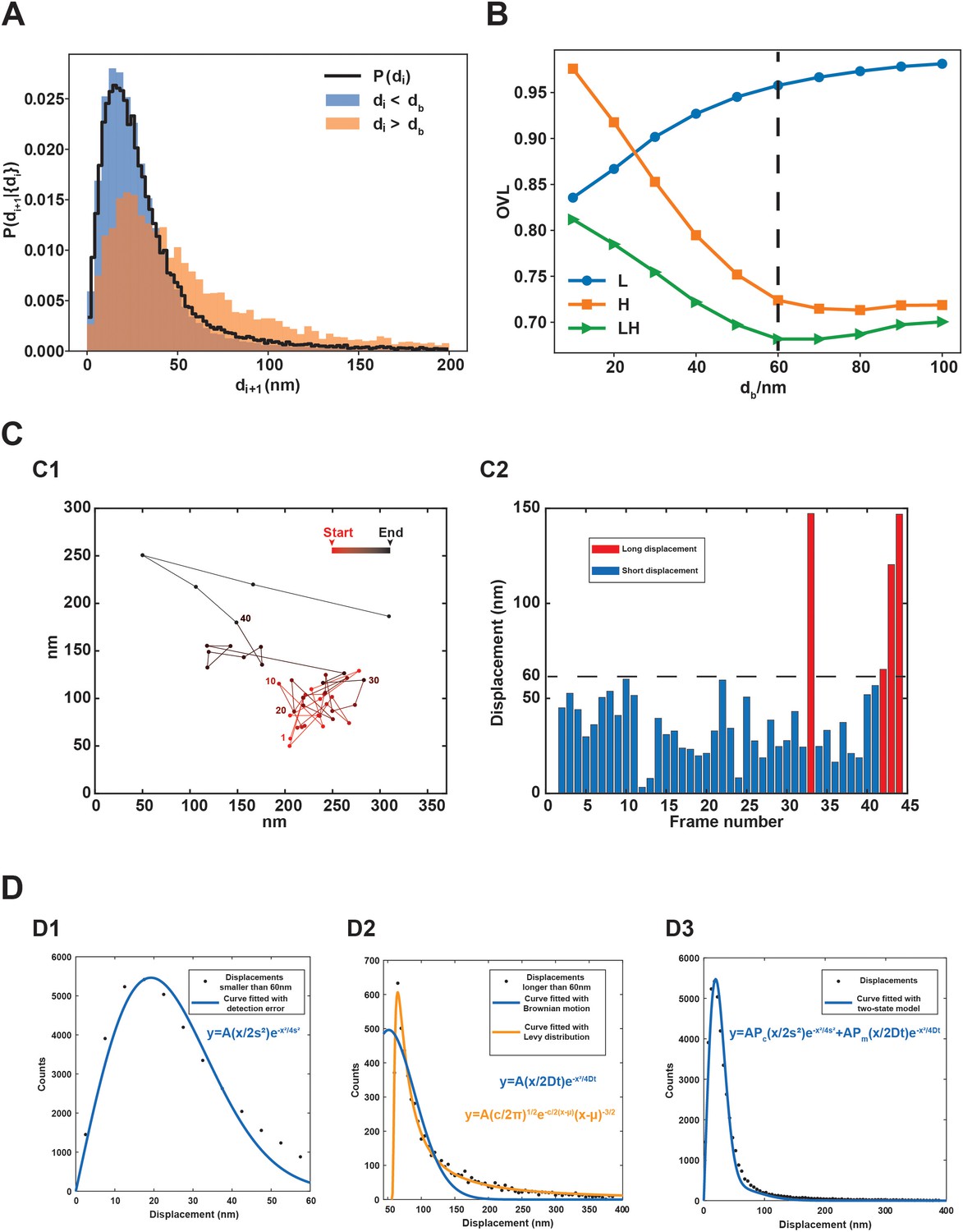
(A) Conditional distribution of a collection of 2522 experimental trajectories with longer than 10 steps with each trajectory residing entirely within a model postsynaptic density (PSD) condensate. P(di+1|{di}) denotes the normalized distribution of the displacement of the (i+1)th step given that the displacement of the ith step belongs to the set {di}. Shown here as examples are P(di+1|di<db) (blue histogram) and P(di+1|di>db) (orange histogram), corresponding to the conditional displacement distributions given that the displacement of the preceding step are, respectively, less than or larger than a chosen boundary value db for demarcating small (low-mobility, L) and large (high-mobility, H) displacements. The conditional distributions shown are for db = 60 nm. The black curve shows the total (unconditional) baseline distribution P(di) obtained from the 2522 experimental condensed-phase tracks considered. For db = 60 nm, the number of di+1 displacements with di < db and di > db are 34,036 and 5286, respectively. Note that the first step of each trajectory is not included in the conditional displacement distributions because it lacks a preceding step. (B) Overlap coefficient (OVL, defined in main text of ‘Materials and methods’) as a function of L-H displacement demarcation value db. Here, the curves labeled by ‘H’ or ‘L’ are OVLs between P(di+1|di > db) or P(di+1|di < db), respectively, and the full (unconditional) displacement distribution P(di); whereas ‘LH’ is the OVLs between the L and H distributions for the same db value. The vertical dashed line indicates the db = 60 nm demarcation, which we regard as optimal for the given set of experimental condensed-phase displacement data. (C) A representative experimentally determined trajectory illustrating an approximate separation of low-mobility and high-mobility displacements. (C1) Time sequence of the trajectory is indicated using color which transitions from red to black from the starting to the end points of the trajectory (changing 25% of redness after every 10 steps) as well as by labels of select position numbers (1, 10, 20, 30, and 40) in the corresponding color. (C2) Bar graphs of frame displacements (in nm) of the trajectory in (C1). To highlight the approximate two-state-like behaviors, short (L) displacements (<60 nm) are shown in blue, whereas long (H) displacements (>60 nm) are shown in red. (D) Black dots: each dot represents displacement counts for bin size of 5 nm. Blue curves: best fits for distribution of displacements smaller than 60 nm (D1) and for displacements longer than 60 nm (D2) with simple Brownian motion as well as best fit for the overall displacements with a two-simple-diffusion-state model (D3). Specifically, the blue curve in each panel is the fitting curve for the given equation shown in blue and was obtained by nonlinear least-squares method using MATLAB. Values for the normalization factor A and fitted parameters are as follows. (D1) A = 172,500, s = 13.6 nm; (D2) A = 41,220,, D = 0.04453 μm2/s; and (D3) A = 185,100, and values of s and D are set to the fitted values in (D1) and (D2). The corresponding square of Pearson correlation coefficient r2 = 0.92, root mean square error (RMSE) = 514.5 for (D1), r2 = 0.91, RMSE = 38.7 for (D2), and r2 = 0.99, RMSE = 18.2 for (D3). In (D2), an optimized fit to a Lévy distribution (orange curve and equation) is included for comparison. The fitted parameters for the Lévy distribution are: A = 37,000,, c = 28.5, and μ = 55.3; the corresponding r2 = 0.99, RMSE = 9.57.
Figure 4 with 2 supplements
Immobilization of molecules by the large dynamic molecular network in the condensed phase of phase-separated systems.
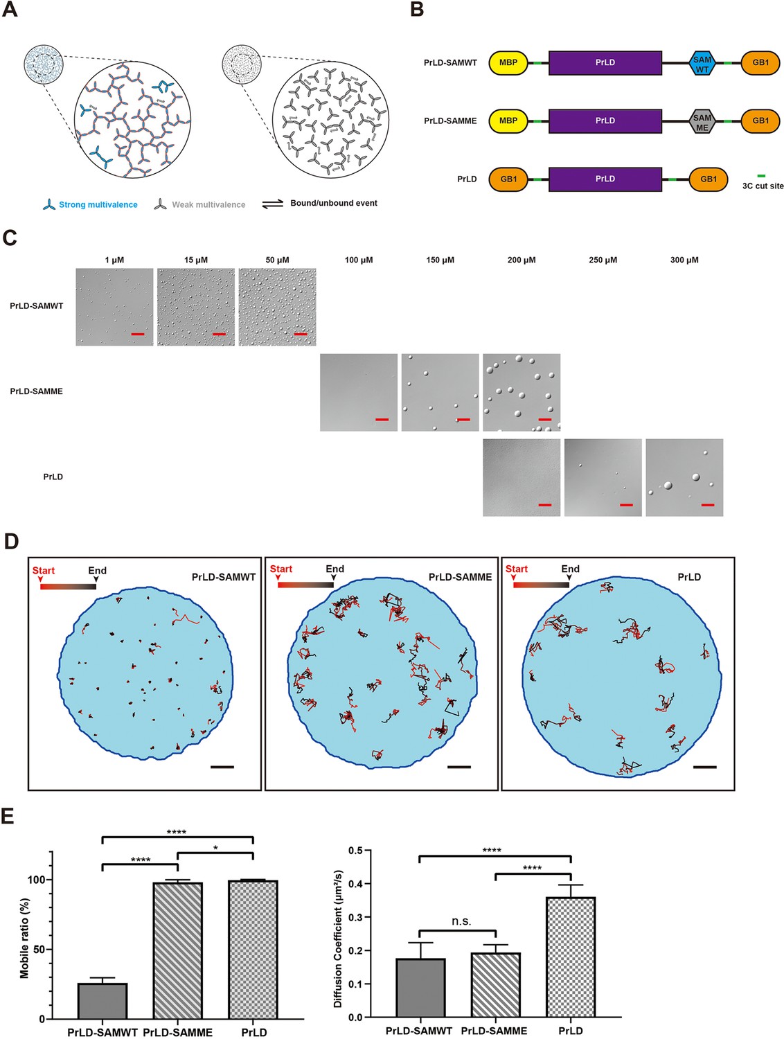
(A) Schematic illustrations of the concept of stable molecular networks in the condensed phase formed by strongly favorable specific and multivalent interactions (left, blue) versus dynamic molecular networks in the condensed phase formed by relatively weak multivalent interactions (right, gray). Red edge highlights a large dynamic (percolated) network. (B) Schematics of the composition of three designed and ‘caged’ single protein phase separation systems with different interaction properties. PrLD, prion-like domain of FUS; SAMWT, WT SAM domain from Shank3; SAMME, the M1718E mutant of Shank3 SAM domain; MBP, maltose binding protein as a caging tag; GB1, the B1 domain of Streptococcal protein G as another caging tag. The HRV-3C cleavage sites (‘3C cut site’) of the proteins are also indicated. (C) DIC images showing phase separations of the three designed proteins at different concentrations after removal of the caging tags by HRV-3C protease cleavage. Scale bar: 20 μm. (D) Representative tracks showing different motion properties of the three designed proteins in condensed phase. Scale bar: 2 μm. Our analysis of diffusion data from the experiments depicted in this figure was based on 2D projections of 3D diffusion tracks. (E) Comparison of Hidden Markov Model (HMM)-estimated mobile ratio in condensed phase (left) and diffusion coefficient in mobile state (right) for the three designed proteins. N = 12, batches of sample with the same condition were used, data are expressed as mean ± standard deviation (SD) with ****p<0.0001, *p<0.0332 by t-test. ‘n.s.’, no significant.
Figure 4—figure supplement 1
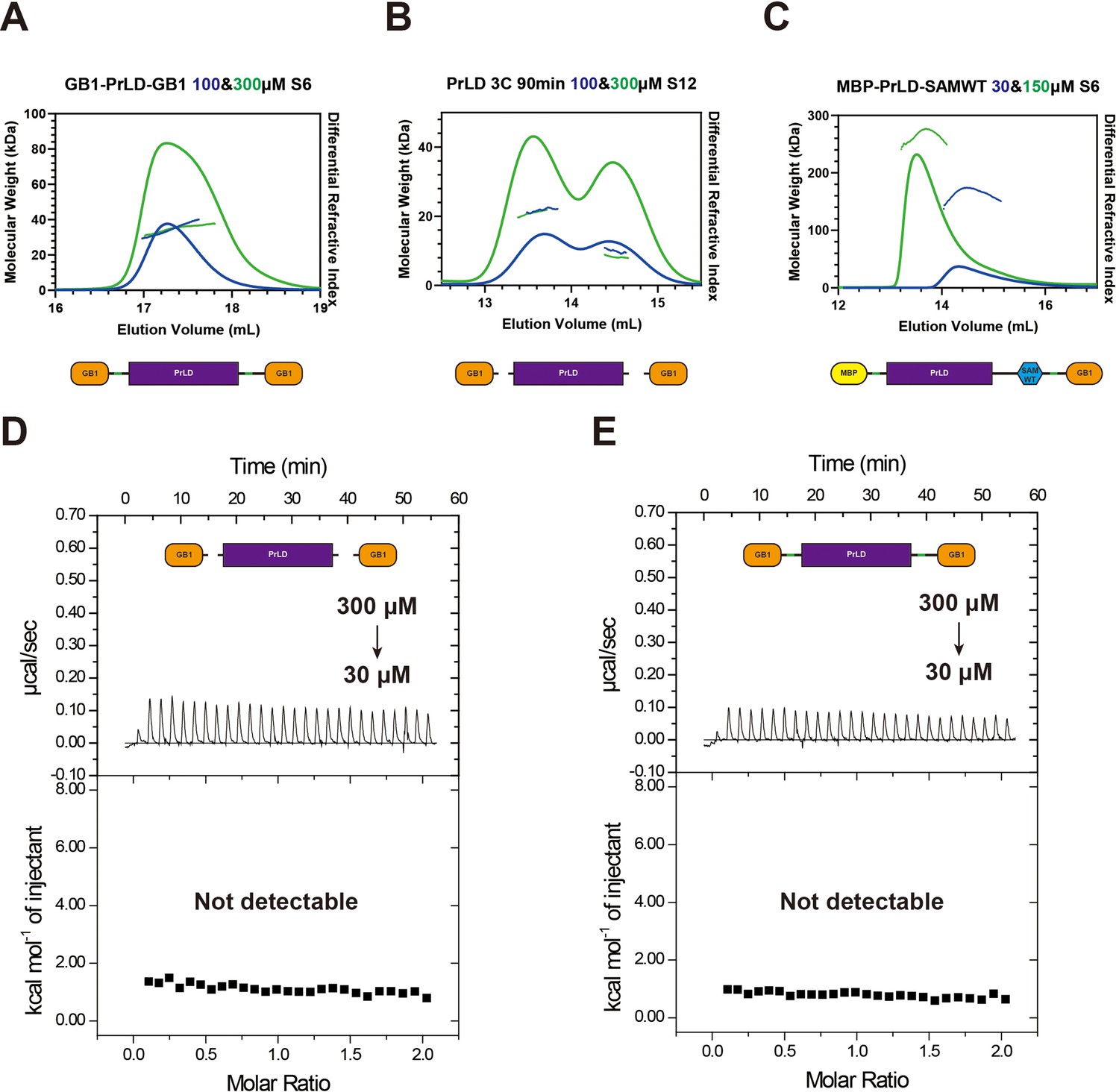
Binding between FUS prion-like domain (PrLD) is extremely weak.
(A) Fast protein liquid chromatography (FPLC)-coupled with static light scattering analysis showing the column behavior and measured molecular weight of the GB1-tagged PrLD at 100 μM (blue curve) and 300 μM (green curve) loading concentrations. (B) FPLC-coupled with static light scattering analysis showing the column behavior and measured molecular weight of the GB1 tag cleaved PrLD at 100 μM (blue curve) and 300 μM (green curve) loading concentrations. (C) FPLC-coupled with static light scattering analysis showing the column behavior and measured molecular weight of the PrLD-SAMWT at 30 μM (blue curve) and 150 μM (green curve) loading concentrations. (D) ITC-based measurements showing undetectable interactions between GB1-tagged PrLD (300 μM titration into 30 μM PrLD in the reaction cell). (E) ITC-based measurements showing undetectable interactions between GB1 tag cleaved PrLD (300 μM titration into 30 μM PrLD in the reaction cell).(Data interpretation) In the system described here, we compared a classical IDR protein fragment, the PrLD of FUS, with the molecular interactions between folded proteins/domain and their targets. On SEC column, GB1-tagged PrLD (theoretical M.W. 37.0 kDa) was eluted at a molecular mass corresponding to a monomer when the loading concentrations of the proteins were at as high as 100 μM (blue curve, measured MW 34.3 ± 0.5 kDa) or 300 μM (green curve, measured MW 35.0 ± 0.9 kDa) in panel (A). To rule out potential impact of the GB1 tag on FUS PrLD interaction, we cleaved the GB1 tag. We took the advantage that tag-cleaved FUS PrLD was stable and monodispersed in solution for up to ~10 hr before phase separation occurs (see Figure 4—figure supplement 2), so we performed SEC-SLS assay of FUS PrLD with the GB1 tag freshly cleaved. The theoretical MW of tag-free FUS PrLD is 22.3 kDa. The measured MW for the tag-free FUS PrLD at the loading concentration of 100 μM (blue curve, measured MW 21.8 ± 3.5 kDa) or 300 μM (green curve. measured MW 20.9 ± 1.1 kDa) also corresponds to the monomer state of the protein in panel (B). As a control, the PrLD-SAMWT fusion protein (theoretical MW 80.7 kDa) was eluted as an oligomer and its elution volumes were heavily dependent on the loading concentrations (loading concentration at 30 μM, blue curve, measured MW 165.0 ± 0.4 kDa; loading concentration at 150 μM, green curve; measured MW 265.0 ± 0.4 kDa) (panel C). We also adopted a thermodynamic-based binding assay using isothermal titration calorimetry (ITC). We titrated 300 μM FUS PrLD (either without or with the GB1 tag cleaved) into 30 μM FUS PrLD in the reaction cell. Again, the ITC-based assay showed that nearly no detectable interactions could be observed between FUS PrLD (panels D, E). These results demonstrate that the interaction between FUS PrLD is very weak, with a Kd value larger than a few hundreds μM based on the experimental methods used here.
Figure 4—figure supplement 2
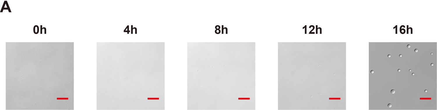
Purified FUS prion-like domain (PrLD) takes more than 12 hr to form condensates.
(A) DIC images showing phase separation of FUS PrLD at different time point after removal of the GB1 tag by HRV-3C protease cleavage. Scale bar: 20 μm.
Figure 5 with 1 supplement
Simulated and experimental fluorescence recovery after photo-bleaching (FRAP) curves of the FUS prion-like domain (PrLD) systems.
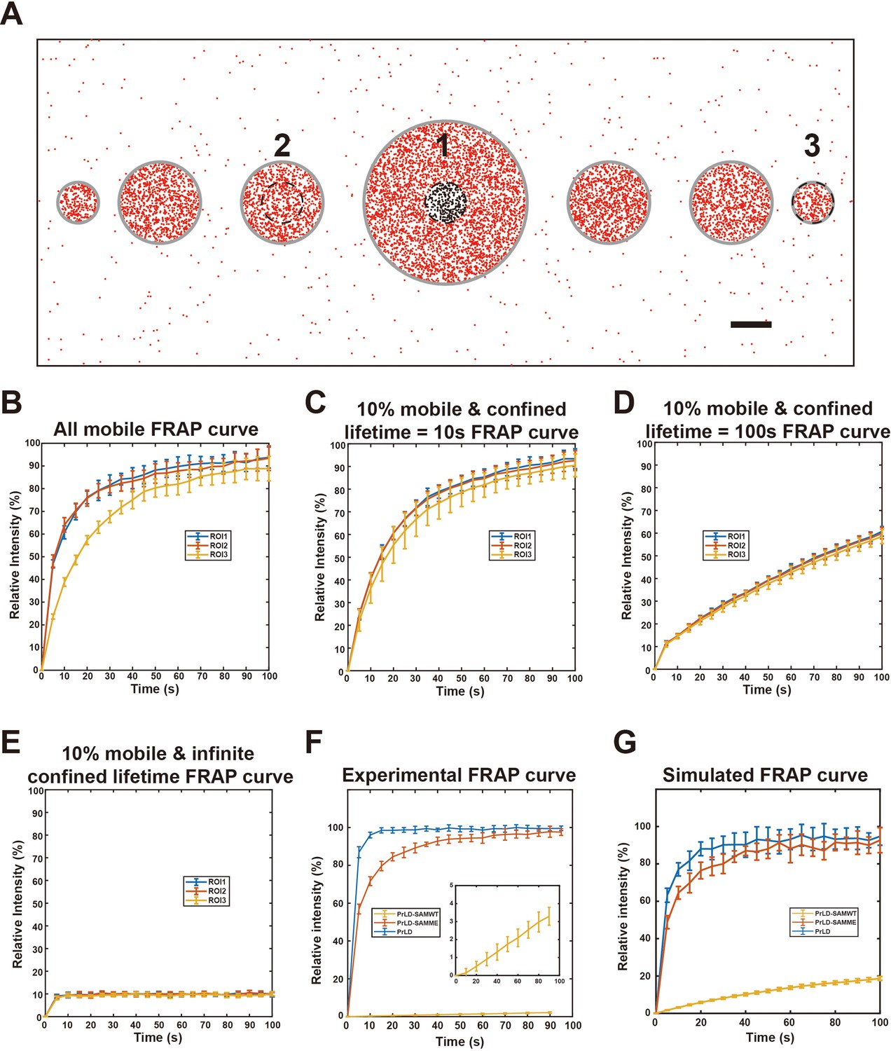
(A) Schematic representation of the phase separation system for the present FRAP simulations. Simulations were conducted in a 20 μm × 8 μm box with periodic boundary conditions. Three regions of interest (ROIs) (1, 2, 3) with a fixed diameter of 0.5 μm are positioned at the center of three different sized droplets (2, 1, and 0.5 μm in diameters, as indicated) were selected for photo-bleaching. Gray lines indicate the phase boundaries of the droplets. Black dots represent bleached molecules that can exchange with unbleached molecules in red. scale bar: 1 μm. (B) Simulated FRAP curves of the three ROIs when all molecules in the condensed phase are mobile, with an enrichment fold of 100 and diffusion coefficients in the condensed and dilute phases being 0.01 μm2/s and 1 μm2/s, respectively. Data are expressed as mean ± standard deviation (SD) from 10 independent simulations. (C) Simulated FRAP curves of the three ROIs when only 10% of molecules in condensed phase are mobile and diffusion coefficients in the condensed and dilute phases being 0.1 μm2/s and 1 μm2/s, respectively. The lifetime of the molecule in the confined state was set at 10 s. (D) Same as in (C) except that the lifetime of the molecules in the confined state was set at 100 s. (E) Same as in (C) except that the molecules in the confined state were treated as permanently immobilized. (F) Experimental FRAP curves of PrLD, PrLD-SAMME, and PrLD-SAMWT condensates. In each case, a photo-bleaching region with the size of 1.95 μm in diameter was selected inside a large droplet (see Figure 5—figure supplement 1). The zoom-in panel is an expanded view of the FRAP curve of PrLD-SAMWT. Data are expressed as mean ± SD, with recovery experiments performed on 10 different droplets. (G) Simulated FRAP curves of the three designed proteins in the condensed phase using the parameters derived from the experiments described in Figure 4 (see ‘Materials and methods’ for quantitative details). The region selected for photo-bleaching has a diameter of 2 μm and is located in a model condensed phase of infinite size. Data are expressed as mean ± SD from 10 independent simulations.
Figure 5—figure supplement 1
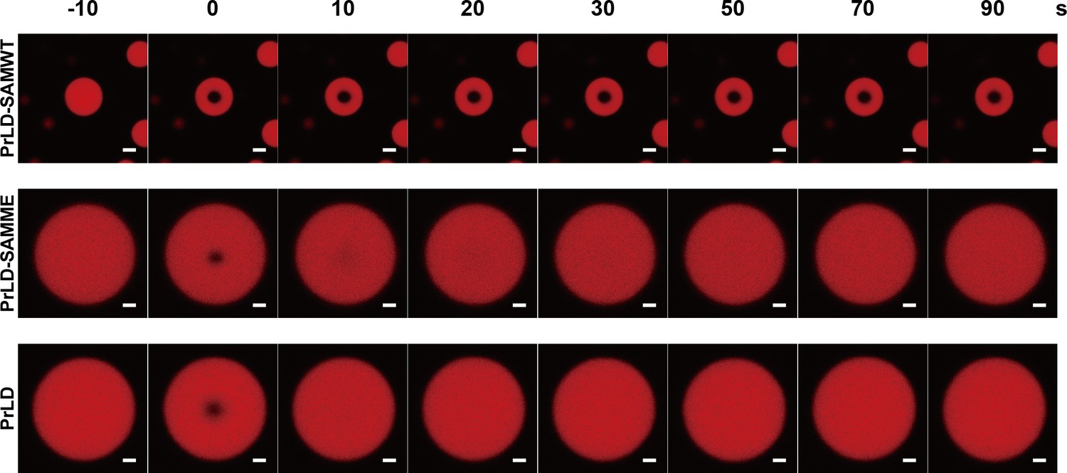
Representative confocal images showing fluorescence recovery after photo-bleaching (FRAP) experiments of the condensed droplets formed by prion-like domain (PrLD), PrLD-SAMME, or PrLD-SAMWT.
The region selected for photo-bleaching has size of 20 pixels or 1.95 μm in diameter. Photo-bleaching started at time point 0. Scale bar: 2 μm.
Author response image 1
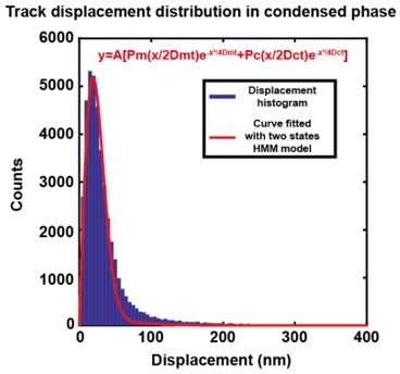
Comparing fitting the experimental molecular displacements with a simple Brownian diffusion model (Figure 3—figure supplement 1C1) against fitting with the optimized HMM two-state diffusion model.
Best fit of the same experimental displacement distribution in condensed phase with a two-state HMM model. Red Curve is the HMM model fit obtained by non-linear least squares method using MATLAB. R2 = 0.98, RMSE = 184.9..
Videos
Video 1
Raw image superimposed with phase boundary and tracks (steps length >5) in the NR2B + postsynaptic density (PSD) phase separation system on 2D supported lipid bilayer (SLB).
Red lines represent tracks in the condensed phase, green lines represent tracks in the dilute phase, and yellow lines represent tracks crossing phase boundaries. Molecules can be seen to switch between a confined state and a mobile state. Molecules are also directly observed to diffuse across phase boundaries. This video is played in real time. Scale bar: 500 nm.
Tables
Table 1
Simulation of phase separations with different input of diffusion parameters.
Monte Carlo method-based simulations of molecular diffusion on supported lipid bilayer (SLB) with experimental phase boundaries. A total of 50,000 molecules were included in each simulation, and these molecules were initially randomly distributed at the beginning of each simulation. Each simulation lasted for 100 s and was independently repeated 10 times. Simulated enrichment fold values were presented as mean value of last 10 s ± SD, where SD is standard deviation for the 10 independent runs.
| Input parameters | Theoretical results | Output results | |||
|---|---|---|---|---|---|
| Dm (μm2/s) | Dd (μm2/s) | Mobile ratio | Mobile state lifetime (s) | Enrichment fold (EF) | Enrichment fold (EF) |
| 0.2 | 0.6 | 0.05 | 0.1 | 60 | 58.9 ± 0.7 |
| 0.1 | 0.6 | 0.1 | 0.1 | 60 | 58.6 ± 0.9 |
| 0.01 | 0.6 | 1 | - | 60 | 57.0 ± 0.8 |
| 0.1 | 0.6 | 0.1 | 0.5 | 60 | 57.9 ± 0.7 |
| 0.1 | 0.6 | 0.05 | 0.1 | 120 | 116.7 ± 1.9 |
| 0.2 | 0.6 | 0.1 | 0.1 | 30 | 29.5 ± 0.3 |
Additional files
Download links
A two-part list of links to download the article, or parts of the article, in various formats.
Downloads (link to download the article as PDF)
Open citations (links to open the citations from this article in various online reference manager services)
Cite this article (links to download the citations from this article in formats compatible with various reference manager tools)
Biological condensates form percolated networks with molecular motion properties distinctly different from dilute solutions
eLife 12:e81907.
https://doi.org/10.7554/eLife.81907


