Modeling single-cell phenotypes links yeast stress acclimation to transcriptional repression and pre-stress cellular states
- Center for Genomic Science Innovation, University of Wisconsin-Madison, United States
- Department of Biomedical Engineering, University of Wisconsin-Madison, United States
- University of Wisconsin Carbone Cancer Center, University of Wisconsin School of Medicine and Public Health, United States
- Department of Medical Genetics, University of Wisconsin-Madison, United States
Figures
Figure 1 with 2 supplements
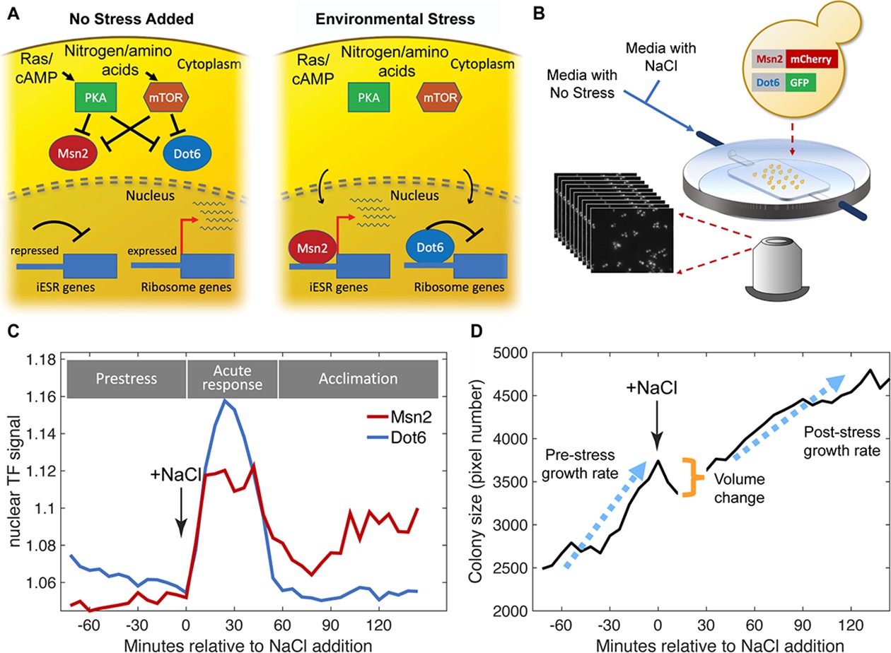
Experimental approach.
(A) Schematic of Msn2 and Dot6 localization in the absence (left) and presence (right) of stress. (B) Diagram of microfluidic device used for time-lapse microscopy. (C) Representative nuclear localization scores (see Methods) for pre-stress growth, the acute-stress response, and the acclimation phase. (D) Cell or two-cell colony size was estimated by the number of pixels within the mask for each colony, and growth rates were calculated based of regression of those points during the pre- or post-stress phases. Cell volume change was reflected in the difference in pixel number before and after stress.
Figure 1—figure supplement 1
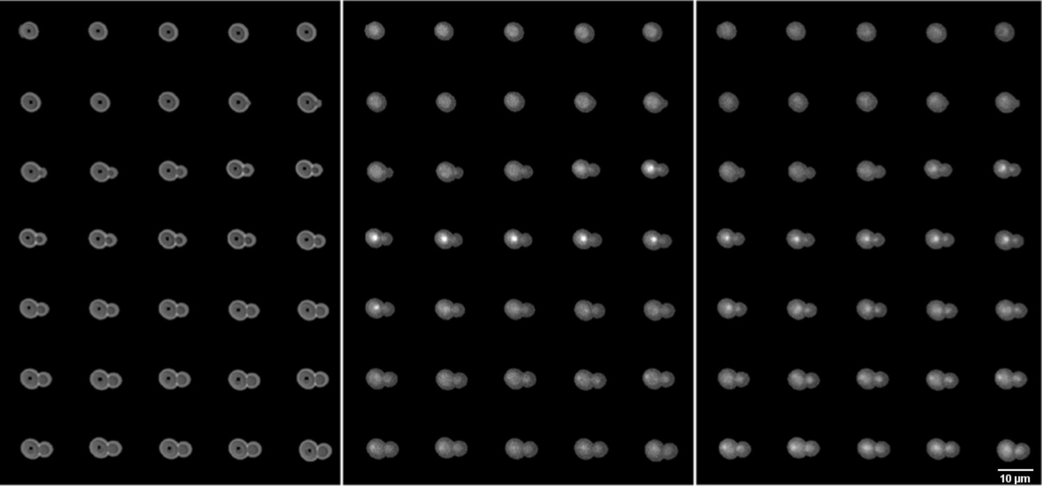
Cellular response to salt within microfluidics device.
Time lapse of a single budding cell expressing Dot6-GFP (center panel) and Msn2-mCherry (right panel) before and after NaCl stress. Halogen images (left panel) were analyzed to identify cells and track them throughout the time course. Images were taken every 6 min, with salt added after 72 min. Top left image is timepoint T1, and timepoints continue from left to right and top to bottom. Salt was added after timepoint T12. The halogen images were used to measure colony size, while the Dot6-GFP and Msn2-mCherry images were used to measure transcription factor nuclear localization. The cell shown is from strain AGY1328; however, it is representative to what was also observed with other strains. For visualization, the brightness of the mCherry channel was increased by 50%.
Figure 1—figure supplement 2
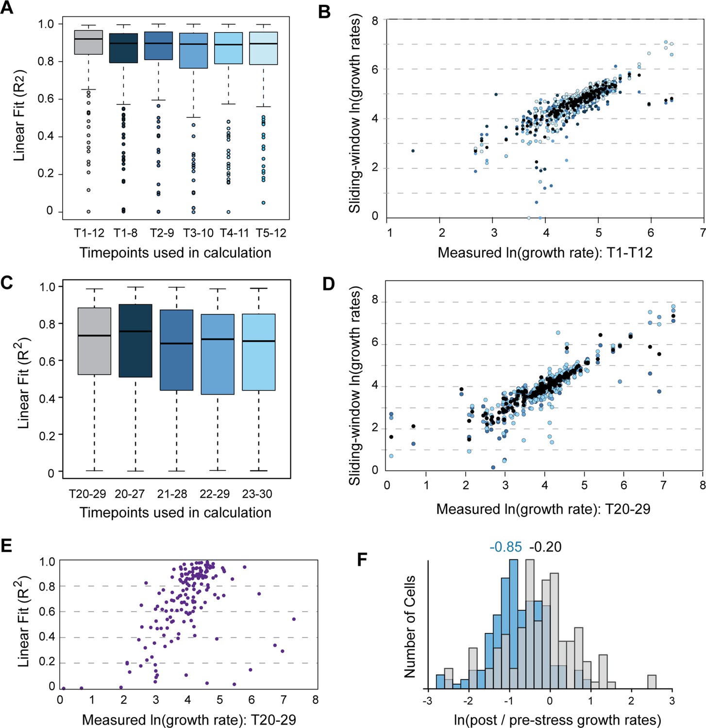
Growth rate estimates are robust.
(A) Growth rate was estimated based from the linear fit of collapsed-image pixel area versus time, from timepoints T1-T12 before addition of salt. The change in pixel area was highly linear for most cells (median R2=0.92, grey box plot). To test the robustness to time points considered, we performed a sliding-window analysis in which growth rates were calculated from subsets of timepoints. The linear fit remained high, and estimated growth rates were well correlated with the growth rates calculated from all pre-stress timepoints. (B) The median of sliding-window growth rates plotted against rates estimated from all timepoints is shown in black, whereas comparisons to sliding-window measurements match the colors from (A). (C–D) Same plots except for post-stress growth rate. As reported in the main text, there was a wider range of growth rates and thus a wider range of linear fits of the data (median R2=0.72). Nonetheless, the measured growth rates were highly correlated with those calculated from sliding windows of fewer timepoints. (E) As might be expected, growth rate of cells that recovered growth after NaCl stress were well estimated by a linear change in colony area, whereas cells that did not recover pre-stress growth rates showed a lower linear fit that was more heavily influenced by noise (confirmed by visual inspection). (F) The reduction in growth rate seen after NaCl treatment (here as in Figure 2B, blue plot) were specific to stress treatment (median ln(growth rate change)=–0.85), since most cells exposed to a shift in media without NaCl (grey bars) showed subtle changes in growth rate (median ln(growth rate change)=–0.20). Together, these analyses show that our estimates of growth rate are robust to time points used and that growth-rate changes discussed in the text are specific to NaCl stress.
Figure 2
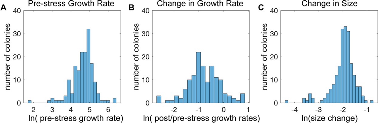
Cell-to-cell heterogeneity in the NaCl stress response.
(A-C) Shown are the distributions of the natural log of (A) colony growth rates before stress, (B) the change in growth rate after NaCl stress compared to before stress, and (C) the maximum change in cell pixel size during the acute-stress response versus during the pre-stress phase.
Figure 3
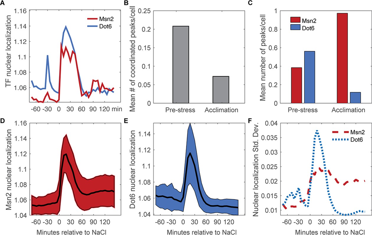
Nuclear translocation dynamics of Msn2 and Dot6 are more coordinated before stress.
(A) Representative traces of Msn2 and Dot6 in the same cell. (B) The average number of coordinated peaks for Msn2 and Dot6, i.e. peaks called within 6 min (1 timepoint) of each other. (C) The average number of nuclear localization peaks per cell for Msn2 (red) and Dot6 (blue) during pre-stress and acclimation phases. (D–E) The average (black line)+/- one standard deviation (colored spread) of Msn2 (D) and Dot6 (E) nuclear localization during the time course. (F) Trace of the standard deviation of nuclear localization over the time course for Msn2 (red) and Dot6 (blue).
Figure 4 with 1 supplement
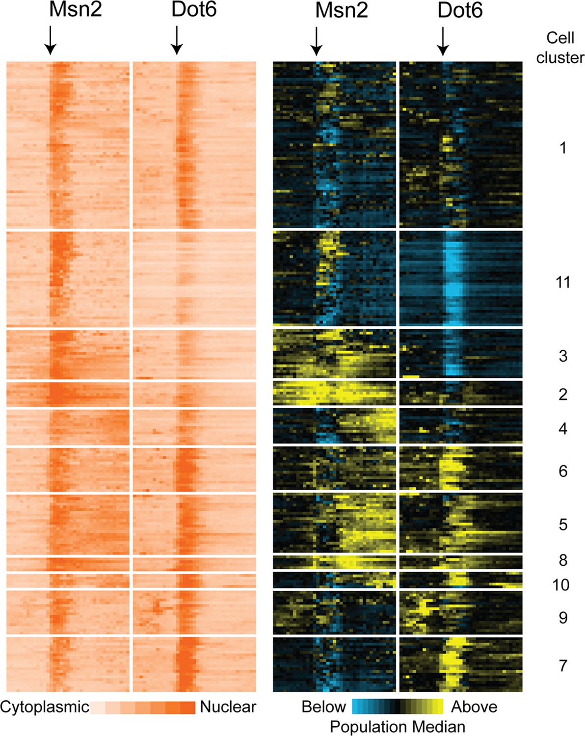
Subpopulations of cells show distinct Msn2 and Dot6 translocation dynamics.
221 cells passing quality control metrics were partitioned into sub clusters based on their population-centered nuclear translocation dynamics shown on the right. Each row represents a cell and each column in a block represents a single timepoint; time of NaCl addition is indicated with an arrow. Data on the left show the log2 ratio of nuclear versus total Msn2 (left) or Dot6 (right) according to the orange-scale key, see Methods. Data on the right show the same data normalized to the population median at each timepoint: yellow values indicate higher-than-median nuclear localization levels and blue indicates lower-than-median nuclear localization. Cell clusters identified by the package mclust are labeled to the right.
-
Figure 4—source data 1
The text file contains the log2 of unnormalized nuclear trace values and the population-median-normalized nuclear trace values across the time course for each cell, divided into clusters (for strain AGY1328).
- https://cdn.elifesciences.org/articles/82017/elife-82017-fig4-data1-v2.zip
Figure 4—figure supplement 1
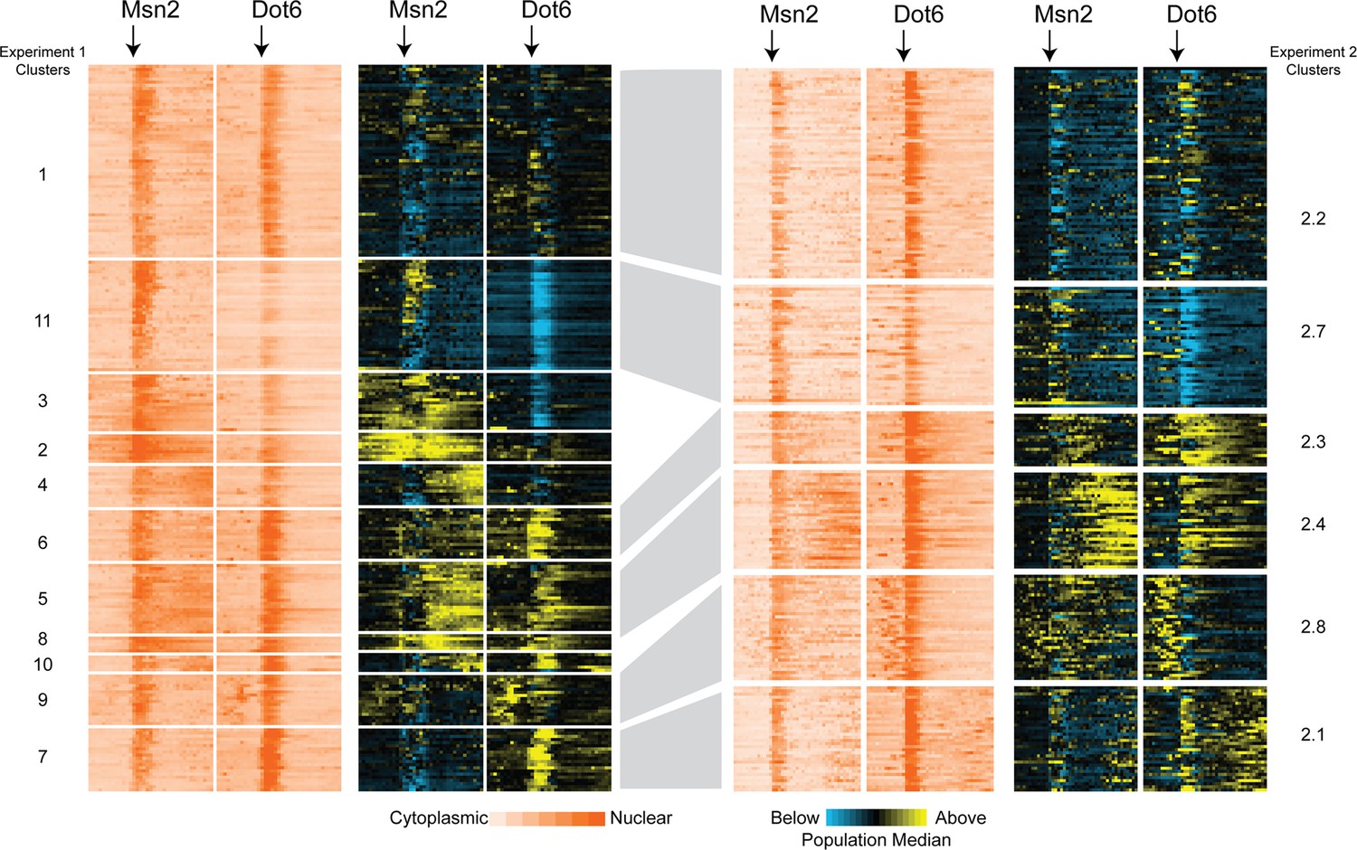
Cellular profiles are recapitulated.
Patterns seen in data from Figure 4 (strain AGY1328, left side) are identifiable in a separate series of triplicated experiments with a second strain (AGY1813: BY4741 Dot6-GFP, Msn-mCherry, Ctt1-iRFP, right side). Data from AGY1813 were clustered independently by mixed-model clustering as described for Figure 4. This analysis identified six clusters of more than three cells (several small clusters were omitted from the figure). Patterns seen in Figure 4 shown on the left were visually identified and aligned with clusters from the second experiment on the right.
-
Figure 4—figure supplement 1—source data 1
The text file contains the log2 of unnormalized nuclear trace values and the population-median-normalized nuclear trace values across the time course for each cell, divided into clusters (for strain AGY1813).
- https://cdn.elifesciences.org/articles/82017/elife-82017-fig4-figsupp1-data1-v2.zip
Figure 5 with 2 supplements
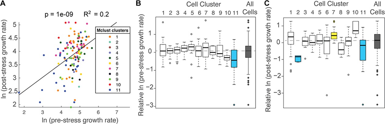
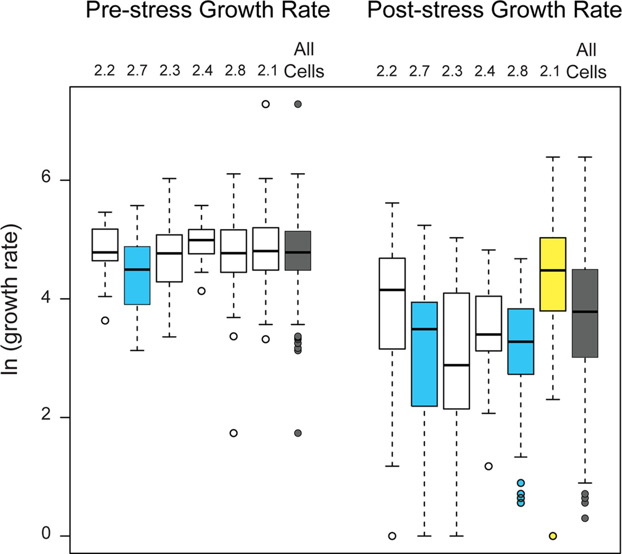
Cell subpopulations display different growth rates before and after stress.
(A) Correlation between the natural log of pre- and post-stress growth rates for each cell, colored according to its cell cluster in Figure 4. (B–C) Distribution of median-centered growth rates before (B) and after (C) NaCl addition, for cell clusters shown in Figure 4. Boxes are colored yellow or blue if the distribution was significantly higher or lower, respectfully, from all other cells in the analysis (Wilcoxon Rank Sum test, FDR < 0.022). Dashed line indicates the median of all cells analyzed.
Figure 5—figure supplement 1
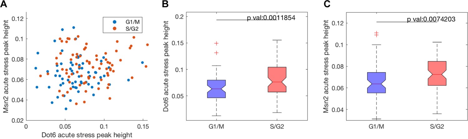
The strength of transcription factor nuclear localization is weakly related to cell cycle phase and budding.
Cells grow the fastest in G1 and M-phase (Goranov et al., 2009), thus cells were binned if they were in G1 or M phase or S/G2 phases at the time of NaCl exposure. (A) The peak height of nuclear localization for Msn2 and Dot6 during the acute-stress phase are plotted, with cells in S/G2 or M/G1 indicated in red or blue, respectively. (B-C) The distribution of acute-stress peak heights for Dot6 (B) or Msn2 (C) was plotted for cells in M/G1 or S/G2. Wilcoxon rank sum tests show that cells in S/G2 had slightly higher nuclear accumulation of both factors (p<0.001).
Figure 5—figure supplement 2
Cell clusters show similar relationships with pre- and post-stress growth rates.
As shown in Figure 5 except for the independent triplicated experiments shown in Figure 4—figure supplement 1. Similar cell clusters show similar relationships in pre- and post-stress growth rates, further confirming that the trends are reproducible across biological replicates, strains, and microscopy conditions.
Figure 6 with 2 supplements
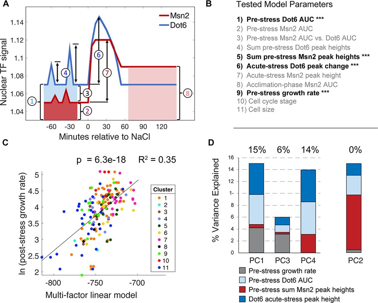
A multi-factor model best explains variation in post-stress growth rate.
(A) A representation of the nuclear localization measurements used in the multi-factor linear regression model. (B) Factors considered in the multi-factor linear regression model; those with significant contributions are highlighted with ***. (C) The variance in ln(post-stress growth rate) explained by the multi-factor linear regression model. P-value and R2 are shown at the top of the plot and cell subcluster is indicated according to the key, showing that no single cluster dominates the correlation. (D) Principal component (PC) regression of post-stress growth rate and deconvolution of contributing factors according to the key. Variance explained is listed at the top of each bar (where PC2 does not contribute to post-stress growth rate).
Figure 6—figure supplement 1
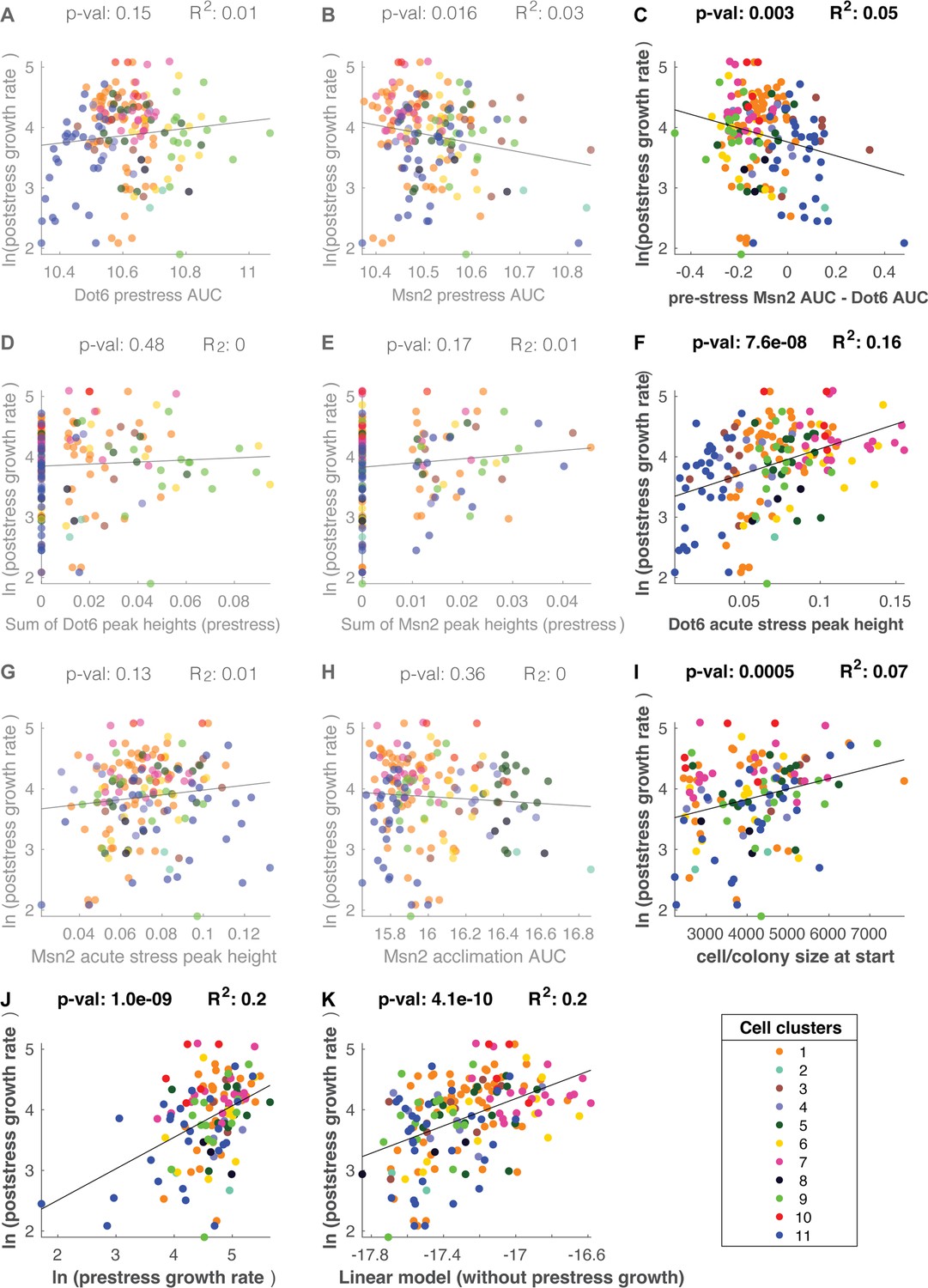
Linear regression of individual parameters on post-stress growth rate.
(A–J) Linear regressions of individual parameters listed in Supplementary file 2. Parameters in which the false discovery rate was <0.025 (p<0.003) are bold whereas other plots are deemphasized. There is a significant fit between cell/colony size at the experiment start time and post-stress growth rate (I); however, this parameter was not significant beyond the multiple-test threshold in the multi-factor linear model (see Supplementary file 3), suggesting that much of cell-size contribution is correlated with and thus absorbed by other factors in the model. (K) Fit from a multiple linear model similar to that shown in Figure 6 except in which pre-stress growth rate was not included (coefficient set to 0).
Figure 6—figure supplement 2
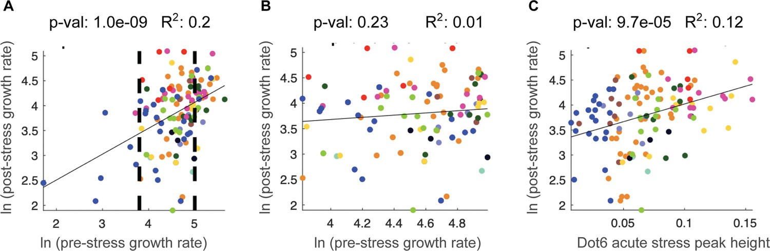
Dot6 acute-stress peak height correlates with post-stress growth rate even across cells with no difference in pre-stress growth.
As an independent approach to disentangle the contribution of Dot6 behavior and pre-stress growth rate, we analyzed only the subset cells that show no difference in pre-stress growth (between dashed lines in A). This subset of cells retains a correlation between Dot6 peak height and post-stress growth rate with nearly the same predictive power (R2=0.12, compare to Figure 6D). (A) Correlation between pre- and post-stress growth rate over all analyzed cells. (B) Same as A except for cells between the dashed lines of A. The figure shows that for this subset of cells, there is no longer a correlation between pre- and post-stress growth rate. (C) Correlation between Dot6 acute-stress peak height and post-stress growth rate for cells shown in B. Cell colors correspond to clusters from Figure 4.
Figure 7 with 1 supplement
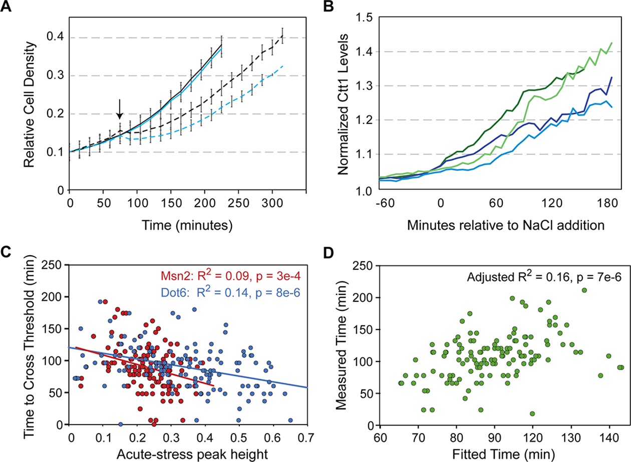
Dot6 activation correlates with faster Ctt1 production.
(A) The average and standard deviation (n=4) of growth rates of wild-type (black lines) and dot6∆tod6∆ cells (blue lines) in the absence (solid) and presence (dashed) of 0.7 M NaCl added at 75 min (arrow). (B) Representative traces of single-cell Ctt1 production for pairs of cells that reach similar levels of Ctt1. (C) Correlation of Ctt1 production timing (time to change 5%) versus acute-stress peak heights. (D) The two-factor model correlates with measured Ctt1 production time, with only marginal contribution of Msn2 peak height (p=0.053). Adjusted R2 is shown in both figures.
Figure 7—figure supplement 1
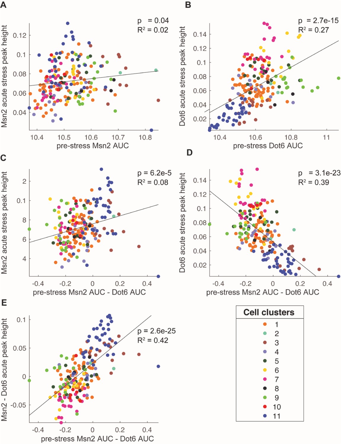
Dot6 acute-stress response is correlated with pre-stress transcription factor behaviors.
We noticed in Figure 4 that many subpopulations showed inverse trends in pre-stress Msn2 versus Dot6 activation. Several clusters that had higher nuclear levels of Dot6 before stress had lower levels of Msn2, and vice versa. We therefore wondered if the relative activation of Dot6 versus Msn2 before stress was any indication of different cellular states. Acute stress peak heights and pre-stress area under the curve (AUC) are as defined in Figure 6B, and cell points are colored according to their cell cluster from Figure 4 as shown in the key. (A–B) Acute-stress peak height plotted against pre-stress AUC for Msn2 (A) or Dot6 (B). (C–E) Acute-stress peak height for Msn2 (C), acute-stress peak height for Dot6 (D), and the difference in acute-stress peak height (E) plotted against the difference in pre-stress AUC. The results show that Dot6 peak height is best explained by the relative pre-stress activation of Msn2 versus Dot6. These differences are likely capturing distinctions about pre-stress cellular states (see Discussion). P-values and R2 of the fit are shown on each plot. All p-values were significant at a Benjamini-Hochberg corrected false discovery rate of 0.05.
Additional files
-
Supplementary file 1
Permutations of coordinately timed peaks in cells in two-cell colonies.
- https://cdn.elifesciences.org/articles/82017/elife-82017-supp1-v2.docx
-
Supplementary file 2
Cell subpopulations are identified in multiple biological replicates.
The number of cells in each mclust cluster from Figure 4 is shown along with the number of those cells from each of three biological replicates. P-values from binomial probability tests (see Methods) are shown and those significant after Holm-Bonferroni correction (namely Cluster 9 which was enriched for cells from replicate 3) are indicated with an asterisk.
- https://cdn.elifesciences.org/articles/82017/elife-82017-supp2-v2.docx
-
Supplementary file 3
Multiple Linear Models: variables, significance, and explained variance.
- https://cdn.elifesciences.org/articles/82017/elife-82017-supp3-v2.docx
-
MDAR checklist
- https://cdn.elifesciences.org/articles/82017/elife-82017-mdarchecklist1-v2.pdf
-
Source code 1
Cell Identification Script.
This MATLAB script takes halogen images and identifies cells. Makes an output file to be used by the 'Source-Code-2.m' script.
- https://cdn.elifesciences.org/articles/82017/elife-82017-code1-v2.zip
-
Source code 2
Cell Tracking Script.
This script takes the output file from Source-Code-1.m and tracks individual cells through time series and extracts cell size and TF nuclear localization.
- https://cdn.elifesciences.org/articles/82017/elife-82017-code2-v2.zip
-
Source data 1
Source data 1 for AGY1328 Single Cell Measurements.
The following is a description of the data within the file ‘Source-Data-1.xls’
Each row represents data for an individual cell from strain AGY1328 (Msn2-mCherry, Dot6-GFP). There are 37 time point measurements in this table, labeled T01 through T37. Each measurement is taken 6 minutes apart (i.e T01 is at the start, T02 is 6 minutes into the experiment, T03 is 12 minutes in, and so on). T01 – T12 represent time points before NaCl is added, T13 through T22 represent the initial acute response to salt, and T23 – T37 represent the acclimated response.
[Column 1] Header: cell_numb
This is the unique identifier for each cell in the dataset.
[Column 2] Header: colony_numb
The colony_numb is different than cell_numb in that if a given cell is part of a two-cell colony, both of these cells in the colony will have the same colony_numb number, but different cell_numb numbers. For example, if two cells are part of colony 3, they will both have a 3 in their colony_numb column. For this dataset, we only analyzed colonies that were either 1 or 2 cells in size at the start of the experiment.
[Column 3] Header: replicate
Which of the three replicate (batch) experiments each cell comes from.
[Columns 4–40] Headers: Msn2_ratio_T01 - Msn2_ratio_T37
[Columns 41–77] Headers: Dot6_ratio_T01 - Dot6_ratio_T37
Data points indicate nuclear_versus_cytoplasmic ratio (average of the top 5% of pixels divided by the median pixel intensity of all pixels in the cell) for Msn2 or Dot6, as indicated in header
[Columns 78–114] Headers: col_size_T01 – col_size_T37
Each values estimates the size of the colony (measured as the number of image pixels that represent the area of a colony).
[Column 115] Header: Pre_stress_growth
Values represent the pre-stress growth rate, measured as the natural log of the rate of increase of colony size through the first 12 time points.
[Column 116] Header: Post_stress_growth
Values represent the post-stress growth rate, measured as the natural log of the rate of increase of colony size through the time points 20–29. The 36 cells removed, as described in the Methods, are NaN.
[Column 117] Header: Maybe_vacuolar
The 18 colonies that had apparent vacuolar localization of Msn2-mCherry during pre-stress time points are noted by ‘1’. All other cells are ‘0’.[Column 118] Header: Pre_str_Msn2_peak_sum
[Column 119] Header: Pre_str_Dot6_peak_sum
These columns contain the sum of called peaks of nuclear localization for prestress time points (see Figure 6 and Methods in main text).
[Column 120] Header: Msn2_AUC_prestress
[Column 121] Header: Dot6_AUC_prestress
[Column 122] Header: Msn2_AUC_acclimation
[Column 123] Header: Dot6_AUC_acclimation
These columns are the ‘Area Under the Curve (AUC) of nuclear localization’ measurements as described in the Methods.
[Column 124] Header: Msn2_acute_peak_height
[Column 125] Header: Dot6_acute_peak_height
These columns contain the ‘Acute Stress Peak Height’ as described in the Methods.
[Column 126] Header: cycle_phase
The cell-cycle phase at the moment of introduction of NaCl stress. This was called from visual inspection of the cells: presence of buds and the location of the nuclei relative to the bud where used to determine the phase: G1, S, G2, M phases. A ‘q’ in the column means that it was questionable what the phase was. A G0 phase is given if there is no evidence for cell division over the entire time course.
- https://cdn.elifesciences.org/articles/82017/elife-82017-data1-v2.xlsx
-
Source data 2
Source Data 2 for AGY1813 Single Cell Measurements.
The following is a description of the data within the file ‘Source-Data-2.xls’.
Each row represents data for an individual cell from strain AGY1813 (Msn2-mCherry, Dot6-GFP, Ctt1-iRFP). There are 45 time point measurements in this table, labeled T01 through T45 for replicates 1 and 2. There are 43 time point measurements in this table, labeled T01 through T43 for replicate 3. Each measurement is taken 6 minutes apart (i.e T01 is at the start, T02 is 6 minutes into the experiment, T03 is 12 minutes in, and so on). T01 – T12 represent time points before NaCl is added, T13 through T22 represent the initial acute response to salt, and T23 – T43/5 represent the acclimated response.
[Column 1] Header: cell_numb
This is the unique identifier for each cell in the dataset.
[Column 2] Header: colony_numb
The colony_numb is different than cell_numb in that if a given cell is part of a two-cell colony, both of these cells in the colony will have the same colony_numb number, but different cell_numb numbers. For example, if two cells are part of colony 3, they will both have a 3 in their colony_numb column. For this dataset, we only analyzed colonies that were either 1 or 2 cells in size at the start of the experiment.
[Column 3] Header: replicate
Which of the three replicate (batch) experiments each cell comes from.
[Columns 4–48] Headers: Msn2_ratio_T01 - Msn2_ratio_T45
[Columns 49–93] Headers: Dot6_ratio_T01 - Dot6_ratio_T45
Data points indicate nuclear_versus_cytoplasmic ratio (average of the top 5% of pixels divided by the median pixel intensity of all pixels in the cell) for Msn2 or Dot6, as indicated in header
[Columns 94–138 ] Headers: Ctt1_norm_T01 – Ctt1_norm_T45
Data point indicate normalized Ctt1 abundance (median pixel intensity of all pixels in the cell normalized by dividing the background median pixel intensity of each image that the cell belonged to).
[Columns 139–183] Headers: col_size_T01 – col_size_T45
Each values estimates the size of the colony (measured as the number of image pixels that represent the area of a colony).
[Column 184] Header: Pre_stress_growth
Values represent the pre-stress growth rate, measured as the natural log of the rate of increase of colony size through time points T02 through T12.
[Column 185] Header: Post_stress_growth
Values represent the post-stress growth rate, measured as the natural log of the rate of increase of colony size through the time points 20–29.
[Column 186] Header: Msn2_AUC_prestress
[Column 187] Header: Dot6_AUC_prestress
[Column 188] Header: Msn2_AUC_acclimation
[Column 189] Header: Dot6_AUC_acclimation
These columns are the ‘Area Under the Curve (AUC) of nuclear localization’ measurements as described in the Methods.
[Column 190] Header: Msn2_acute_peak_height
[Column 191] Header: Dot6_acute_peak_height
These columns contain the ‘Acute Stress Peak Height’ as described in the Methods.
[Column 192] Header: Ctt1_peak_height_max
This column contains the maximum Ctt1 levels (the maximum fluorescent signal from T12 through T43 timepoint minus the median of the pre-stress T1 through T11 signal), as described in the methods.
[Column 193] Header: Ctt1_time_to_cross_threshold(min)
This column contains the time it took for each cell to cross a 5% change in Ctt1 abundance, as described in the methods. Cells that did not cross that threshold were not included in the timing analysis and that column was left blank for those cells.
- https://cdn.elifesciences.org/articles/82017/elife-82017-data2-v2.xlsx
Download links
A two-part list of links to download the article, or parts of the article, in various formats.
Downloads (link to download the article as PDF)
Open citations (links to open the citations from this article in various online reference manager services)
Cite this article (links to download the citations from this article in formats compatible with various reference manager tools)
Modeling single-cell phenotypes links yeast stress acclimation to transcriptional repression and pre-stress cellular states
eLife 11:e82017.
https://doi.org/10.7554/eLife.82017


