Misstatements, misperceptions, and mistakes in controlling for covariates in observational research
- Department of Epidemiology and Biostatistics, Indiana University School of Public Health-Bloomington, United States
- Department of Applied Health Science, Indiana University School of Public Health-Bloomington, United States
- Department of Statistics and Data Science, Southern Methodist University, United States
- University of Memphis, School of Public Health, United Kingdom
Figures
Figure 1
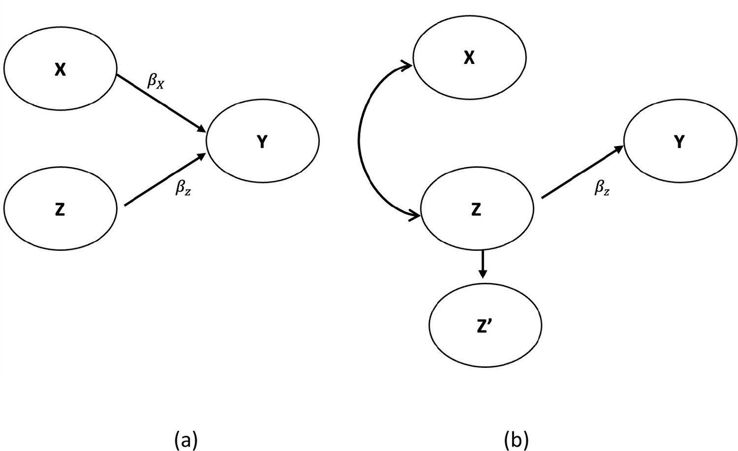
Agree (a) vs. disagree (b) with the interpretation of Misperception 5a.
Demonstrates a nonlinear and non-monotonic association between body mass index (BMI) and mortality among U.S. adults aged 18–85 years old. This figure suggests that BMI ranging between 23–26 kg/m2 formed the nadir of the curve with the best outcome while persons with BMI levels below or above the nadir of the curve experienced increased mortality on average. Source: (Fontaine et al., 2003).
Figure 2

Association between body mass index and hazard ratio for death among U.S. adults aged 18–85 years old.
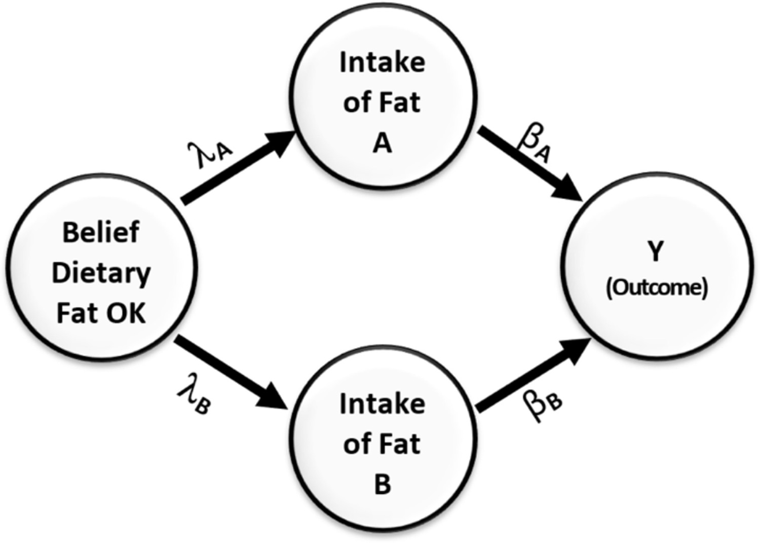
Figure 3

Causal relationships of health outcome, dietary fat consumption, and the belief that consumption of dietary fat is not dangerous.
Direction of arrows represents causal directions and λA, λB, βA, and βB are structural coefficients.
Figure 4
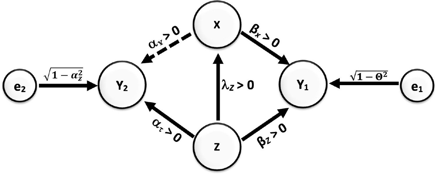
Causal relationships of outcome, covariate, and potentially biasing covariate (PBC).
Direction of arrows represents causal directions and λz, αz, αx, βz, and βx are structural coefficients. The error terms e1 and e2 have variances chosen so Y1 and Y2 have variances 1 (see the Appendices for more details).
Appendix 1—figure 1
Causal relationships of health outcome, dietary fat consumption, and the belief that consumption of dietary fat is not dangerous.
Direction of arrows represents causal directions and 𝜆A, 𝜆B, 𝛽A, and 𝛽B are structural coefficients.
Appendix 2—figure 1
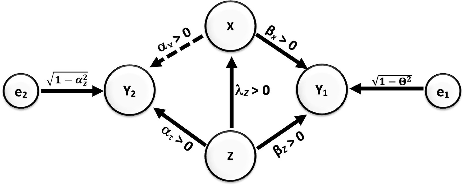
Causal relationships of outcome, covariate, and confounding.
Direction of arrows represents causal directions and 𝜆z, 𝛼z, 𝛼x, 𝛽z, and 𝛽x are structural coefficients.
Appendix 2—figure 2
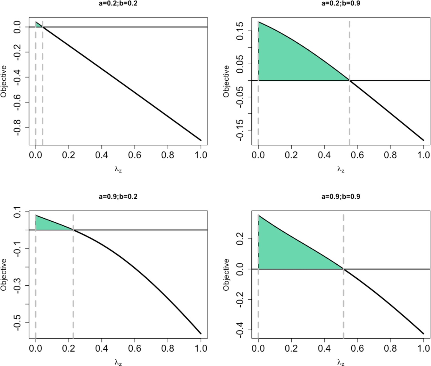
Possible values of based on each choice of the pairs of a, b.
The area shaded in green denotes the area for which a value has a value τ that makes Equation 13 equal zero.
Tables
Appendix 1—table 1
Parameters used to generate simulated data for the simulation studies under Misperception 9.
| Scenario | βA | βB | λA | λB | |||
|---|---|---|---|---|---|---|---|
| I | –0.4 | 0.3 | 0.93 | 0.25 | 0.25 | ||
| II | 0.4 | –0.3 | 0.93 | 0.25 | 0.25 | ||
| III | –0.5 | 0.24 | 0.8 | 0.6 | 0.8076 | 0.36 | 0.64 |
| IV | 0.5 | –0.24 | 0.8 | 0.6 | 0.8076 | 0.36 | 0.64 |
Appendix 1—table 2
Summary of bias when fitting the full model (𝑀𝐹) and the reduced model (MR).
The bias is defined as , where is the least-squares estimate under the corresponding model.
| Scenario | n=500 | n=1000 | n=2000 | |||
|---|---|---|---|---|---|---|
| MF | MR | MF | MR | MF | MR | |
| I | –0.0007 | 0.2248 | 0.0001 | 0.2251 | –0.0001 | 0.2249 |
| II | 0.0005 | –0.2249 | 0.0003 | –0.2249 | 0.0002 | –0.2248 |
| III | –0.0001 | 0.24 | 0.0003 | 0.2405 | –0.0003 | 0.2399 |
| IV | 0.0004 | –0.2396 | –0.0002 | –0.24 | –0.0005 | –0.2402 |
Appendix 2—table 1
The correlation matrix among Z, X, Y2, and Y1 without selecting on Y1.
| Z | X | Y2 | Y1 | |
|---|---|---|---|---|
| Z | 1 | |||
| X | 1 | |||
| Y2 | 1 | |||
| Y1 | 1 |
Appendix 2—table 2
The squared correlation and slope of regression.
| Quantity of interest | Without selection on Y1 | With selection on Y1 |
|---|---|---|
| Squared (zero-order) correlation of X and Y2 | ||
| Squared (partial) correlation of X and Y2, controlling for Z | ||
| Slope of univariable regression of Y2 on X | ||
| Partial slope of regression of Y2 on X, controlling for Z |
Appendix 2—table 3
Estimated Average Bias of Under Various Scenarios.
Where are selected to Induce a Zero Correlation Between and After Selecting on . Results are based on sample size of n=50,000 and 1000 samples obtained from the data-generating model described above.
| All data | Select on | |||||||||
|---|---|---|---|---|---|---|---|---|---|---|
| 0.2 | 0.2 | 0.0422 | 0.2000 | 0.1952 | 0.0200 | –0.5774 | –0.0000 | 0.0118 | –0.0002 | –0.0002 |
| 0.2 | 0.2 | 0.0422 | 0.1999 | 0.1946 | 0.0350 | 1.3809 | –0.0001 | 0.0208 | –0.0004 | –0.0008 |
| 0.2 | 0.9 | 0.5519 | 0.1931 | 0.8361 | 0.2700 | 0.4647 | –0.0001 | 0.1620 | –0.0002 | –0.0001 |
| 0.2 | 0.9 | 0.5519 | 0.1857 | 0.8175 | 0.4000 | 1.8276 | –0.0001 | 0.2398 | –0.0002 | –0.0003 |
| 0.9 | 0.2 | 0.2277 | 0.8936 | 0.0683 | 0.1200 | 0.6717 | 0.0001 | 0.0721 | 0.0005 | 0.0009 |
| 0.9 | 0.2 | 0.2277 | 0.8842 | 0.0598 | 0.1900 | 3.0584 | 0.0001 | 0.1140 | –0.0080 | –0.0118 |
| 0.9 | 0.9 | 0.5156 | 0.8710 | 0.2383 | 0.2600 | –0.1627 | –0.0002 | 0.1556 | –0.0001 | –0.0003 |
| 0.9 | 0.9 | 0.5156 | 0.8207 | 0.1818 | 0.4500 | 2.3590 | –0.0002 | 0.2699 | 0.0011 | –0.0005 |
Download links
A two-part list of links to download the article, or parts of the article, in various formats.
Downloads (link to download the article as PDF)
Open citations (links to open the citations from this article in various online reference manager services)
Cite this article (links to download the citations from this article in formats compatible with various reference manager tools)
Misstatements, misperceptions, and mistakes in controlling for covariates in observational research
eLife 13:e82268.
https://doi.org/10.7554/eLife.82268


