Retinal motion statistics during natural locomotion
- Center for Perceptual Systems, The University of Texas at Austin, United States
- Department of Biology, Northeastern University, United States
- School of Optometry, Indiana University, United States
Figures
Figure 1
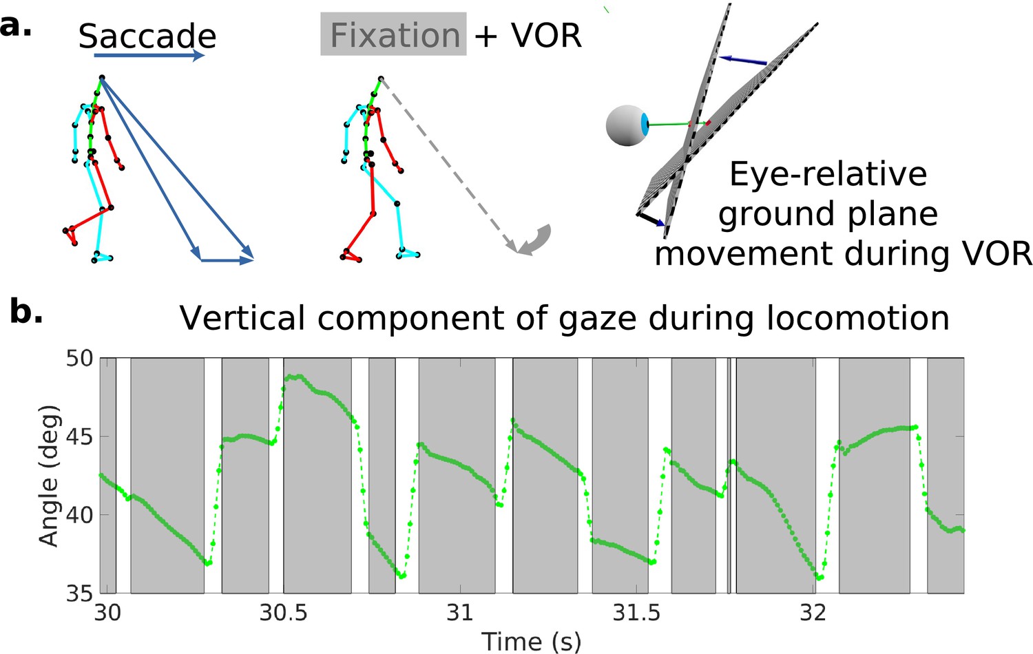
Characteristic oculomotor behavior during locomotion.
(a) Schematic of a saccade and subsequent gaze stabilization during locomotion when looking at the nearby ground. In the top left, the walker makes a saccade to an object further along the path. In the middle panel, the walker fixates (holds gaze) at this location for a time. The right panel shows the gaze angle becoming more normal to the ground plane during stabilization. (b) Excerpt of vertical gaze angle relative to gravity during a period of saccades and subsequent stabilization. As participants move forward while looking at the nearby ground, they make sequences of saccades (indicated by the gaps in the trace) to new locations, followed by fixations where gaze is held stable at a location in the world while the body moves forward along the direction of travel (indicated by the lower velocity green traces). The higher velocity saccades were detected as described in the text based on both horizontal and vertical velocity and acceleration. These are followed by slower counter-rotations of the eye in the orbit in order to maintain gaze at a fixed location in the scene (the gray time slices).
Figure 2
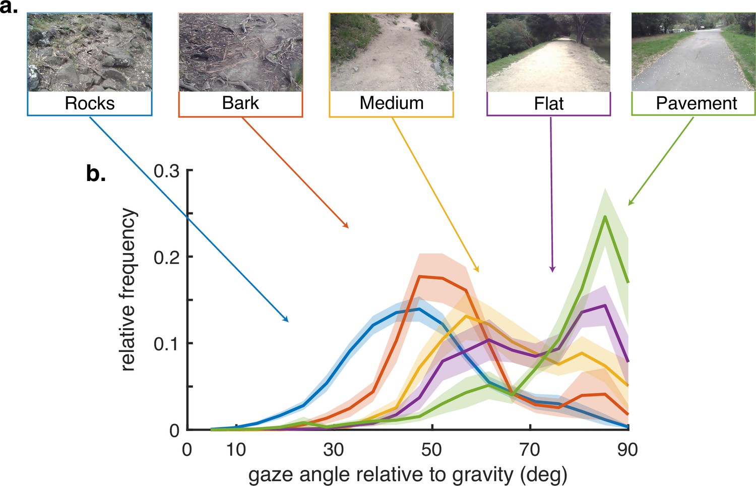
Gaze behavior depends on terrain.
(a) Example images of the five terrain types. Sections of the hiking path were assigned to one of the five terrain types. The Pavement terrain included the paved parts of the hiking path, while the Flat terrain included the parts of the trail which were composed of flat packed earth. The Medium terrain had small irregularities in the path as well as loose rocks and pebbles. The Bark terrain (though similar to the Medium terrain) was given a separate designation as it was generally flatter than the Medium terrain but large pieces of bark and occasional tree roots were strewn across the path. Finally, the Rocks terrain had significant path irregularities which required attention to locate stable footholds. (b) Histograms of vertical gaze angle (angle relative to the direction of gravity) across different terrain types. In very flat, regular terrain (e.g. pavement, flat) participant gaze accumulates at the horizon (90°). With increasing terrain complexity participants shift gaze downward (30°–60°). Data are averaged over 10 subjects for rocky terrain and 8 subjects for the other terrains. Shaded error bars are ±1 SEM. Individual subject data are shown in ‘Methods’.
Figure 3
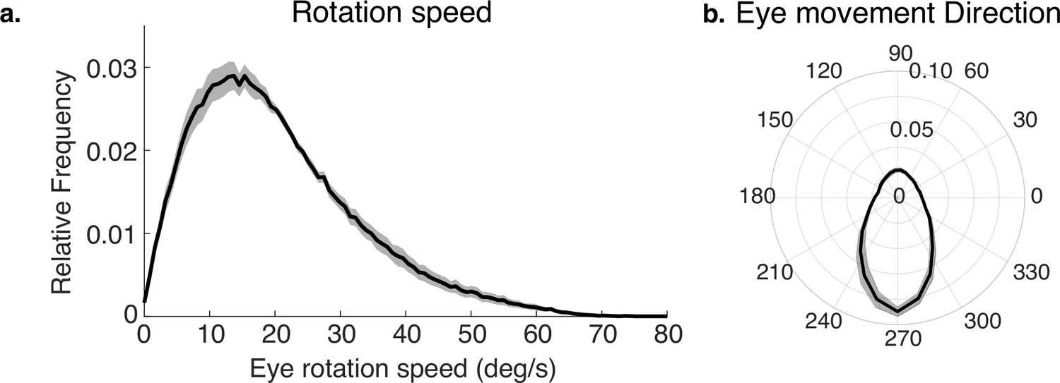
Eye rotations during stabilization.
(a) The distribution of speeds during periods of stabilization (i.e. eye movements that keep point of gaze approximately stable in the scene). (b) A polar histogram of eye movement directions during these stabilizing movements. 270 deg corresponds to straight down in eye centered coordinates, while 90 deg corresponds to straight up. Stabilizing eye movements are largely in the downward direction, reflecting the forward movement of the body. Some upward eye movements occur and may be due to misclassification of small saccades or variation in head movements relative to the body. Shaded region shows ±1 SEM across 10 subjects.
Figure 4
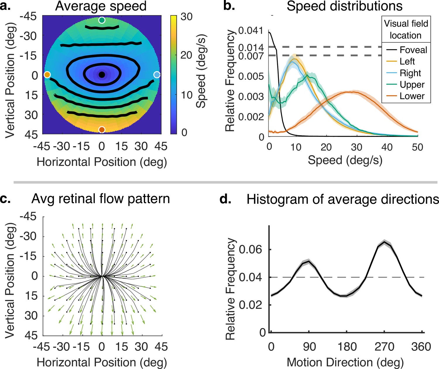
Speed and direction of retinal motion signals as a function of retinal position.
(a) Average speed of retinal motion signals as a function of retinal position. Speed is color mapped (blue = slow, red = fast). The average is computed across all subjects and terrain types. Speed is computed in degrees of visual angle per second. (b) Speed distributions at five points in the visual field at the fovea and four cardinal locations. The modal speed increases in all four cardinal locations, though more prominently in the upper/lower visual fields. Speed variability also increases in the periphery in comparable ways. (c) Average retinal flow pattern as a function of retinal position. The panel shows the integral curves of the flow field (black) and retinal flow vectors (green). Direction is indicated by the angle of the streamline drawn at particular location. Vector direction corresponds to the direction in a 2D projection of visual space, where eccentricity from the direction of gaze in degrees is mapped linearly to distance in polar coordinates in the 2D projection plane. (d) Histogram of the average retinal motion directions (in c) as a function of polar angle. Error bars in (b) and (d) are ±1 SEM over 9 subjects.
Figure 5

Effect of vertical gaze angle on retinal motion speed and direction.
This analysis compares the retinal motion statistics for upper (60°–90°) vs. lower vertical gaze angles (17°–45°). The upper vertical gaze angles correspond to far fixations while the lower vertical gaze angles correspond to fixations closer to the body. (a) Average motion speeds across the visual field. (b) Five example distributions are shown as in Figure 4. Looking at the ground near the body (i.e. lower vertical gaze angles) reduces the asymmetry between upper and lower visual fields. Peak speeds in the lower visual field are reduced, while speeds are increased in the upper visual field. (c) Average retinal flow patterns for upper and lower vertical gaze angles. (d) Histograms of the average directions plotted in (c). While still peaking for vertical directions, the distribution of directions becomes more uniform as walkers look to more distant locations. Data are pooled across subjects.
Figure 6
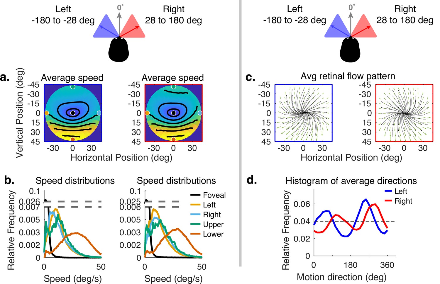
Effect of horizontal gaze angle on motion speed and direction.
Horizontal gaze angle is measured relative to the head translation direction. (a) Average retinal motion speeds across the visual field. (b) Five distributions sampled at different points in the visual field, as in Figure 4. The effect of horizontal gaze angle on retinal motion directions is unremarkable, except for a slight tilt in to contour lines. (c) Average retinal flow patterns for leftward and rightward gaze angles. (d) Histograms of the average directions plotted in (c). These histograms demonstrate the shift of the rotational component of the flow field. Data are pooled across subjects.
Figure 7
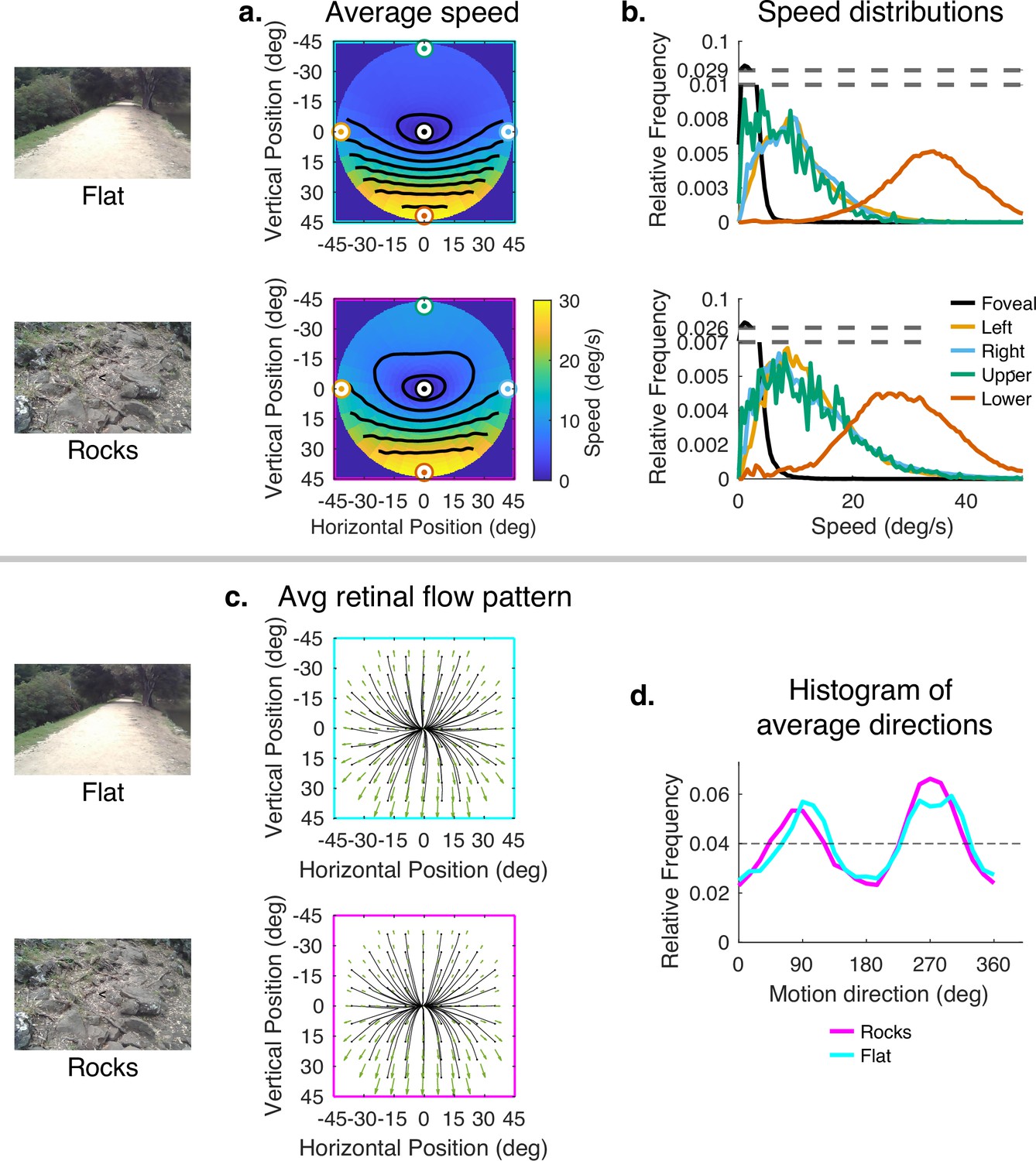
Effect of terrain (controlling for vertical gaze) on retinal motion direction and speed.
While the vertical field asymmetry is slightly greater for the flat terrain, the effects of terrain on retinal motion direction and speed are modest. (a) Average retinal motion speeds across the visual field. (b) Five distributions sampled at different points in the visual field, as in Figure 4. (c) Average retinal flow patterns for leftward and rightward gaze angles. (d) Histograms of the average directions plotted in (c). Data are pooled across subjects.
Figure 8
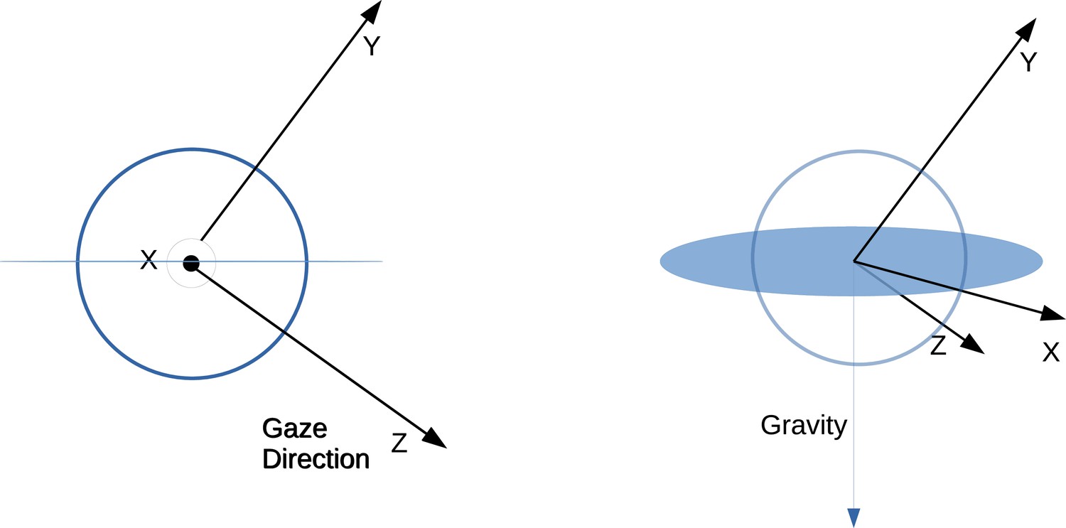
Schematic depicting eye relative coordinate system.
Left and right show basis vectors used from different viewpoints. Z corresponds to the gaze direction in world coordinates. Then X is the vector perpendicular to both Z and the gravity vector. Finally, the Y coordinate is the vector perpendicular to both X and Z. The X vector thus resides within the plane perpendicular to gravity.
Figure 9

Sample of the terrain reconstruction is rendered as RGB image showing the level of detail provided by the photogrammetry.
Figure 10

Retinal image slippage.
Normalized relative frequency histogram of the deviation from the location of the initial fixation over the course of a fixation. Initial fixation location is computed and tracked over the course of each fixation, and compared to current fixation for duration of each fixation. Median deviation value is calculated for each fixation. The histogram captures the extent of variability of initially fixated locations relative to the measured location of the fovea over the course of fixations, with most initially fixated locations never deviating more than 2 deg of visual angle during a fixation.
Figure 11
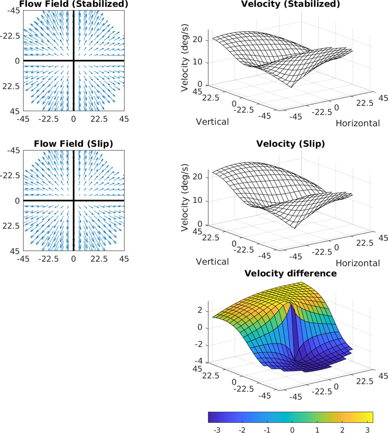
Effects of 3.2 deg/s slip on velocity.
The median slip of approximately 0.8 deg during a 250 ms fixation would lead to a retinal velocity of 3.2 deg/s at the fovea. The figure shows how retinal slip of this magnitude would affect speed distributions across the retina. The flow fields in the two cases (perfect stabilization and 0.8 deg of slip) are shown on the left, and the speed distributions are shown on the right. The bottom plot shows a heat map of the difference.
Figure 12

Speed and direction distributions for saccades.
The distribution of angular velocities of the eye during saccadic eye movements is shown on the left. On the right is a 2D histogram of vertical and horizontal components of the saccades.
Figure 13

Effect of saccades on speed distributions.
Figure 14

Individual participant data – compare to Figure 2.
Histograms of vertical gaze angle (angle relative to the direction of gravity) across different terrain types. In very flat, regular terrain (e.g. pavement, flat) participant gaze accumulates at the horizon (90°). With increasing terrain complexity, participants shift gaze downward (30°–60°). A total of 10 participants are shown. Participants A1–2 correspond to two participants whose data was collected in Austin, TX. The data from these participants includes only the ‘rocks’ terrain. B3–B10 correspond to eight participants whose data was collected in Berkeley, CA.
Figure 15

Individual participant data – compare to Figure 4 (five participants: A1–A2, B3–B5).
Column 1: average speed of retinal motion signals as a function of retinal position. Speed is color mapped (blue = slow, red = fast). The average is computed across all subjects and terrain types. Speed is computed in degrees of visual angle per second. Column 2: speed distributions at five points in the visual field (the fovea and four cardinal locations). Column 3: average retinal flow pattern. Column 4: Histogram of the average retinal motion directions (Column 3) as a function of polar angle.
Figure 16
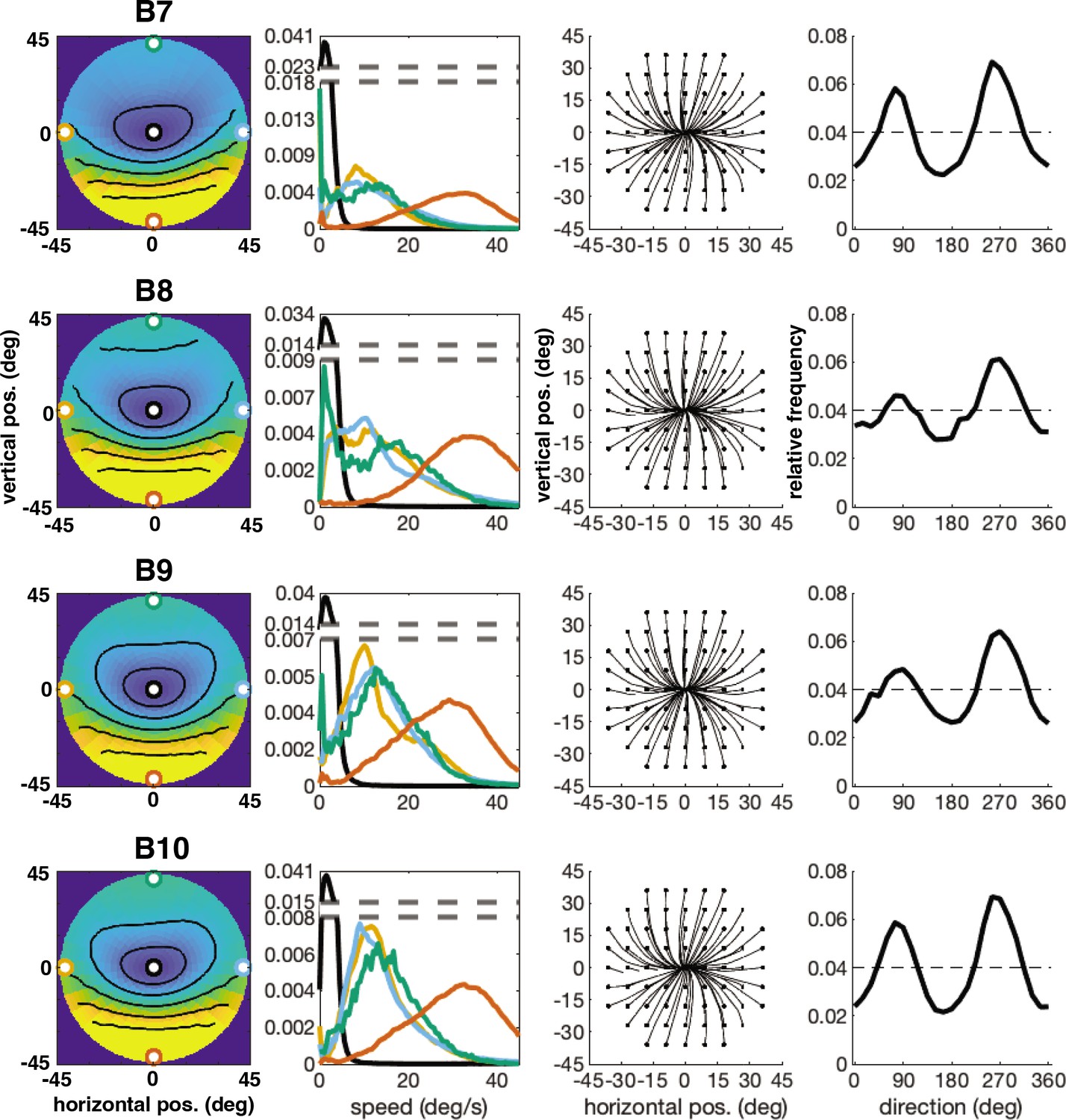
Individual participant data – compare to Figure 4 (five participants: B6–B10).
Column 1: average speed of retinal motion signals as a function of retinal position. Speed is color mapped (blue = slow, red = fast). The average is computed across all subjects and terrain types. Speed is computed in degrees of visual angle per second. Column 2: speed distributions at five points in the visual field (the fovea and four cardinal locations). Column 3: average retinal flow pattern. Column 4 Histogram of the average retinal motion directions (in Column 3) as a function of polar angle. Note: B6’s data is absent because the angle of head camera during data collection precluded proper estimates of retinal flow across the visual field and resulted in poor terrain reconstruction.
Videos
Video 1
Gaze behavior during locomotion.
Visualization of visual input and eye and body movements during natural locomotion.
Video 2
Visual motion during locomotion.
Visualization of eye and head centered visual motion during natural locomotion.
Additional files
Download links
A two-part list of links to download the article, or parts of the article, in various formats.
Downloads (link to download the article as PDF)
Open citations (links to open the citations from this article in various online reference manager services)
Cite this article (links to download the citations from this article in formats compatible with various reference manager tools)
Retinal motion statistics during natural locomotion
eLife 12:e82410.
https://doi.org/10.7554/eLife.82410


