Position representations of moving objects align with real-time position in the early visual response
- University of Melbourne, Australia
- University of Amsterdam, Netherlands
Figures
Figure 1
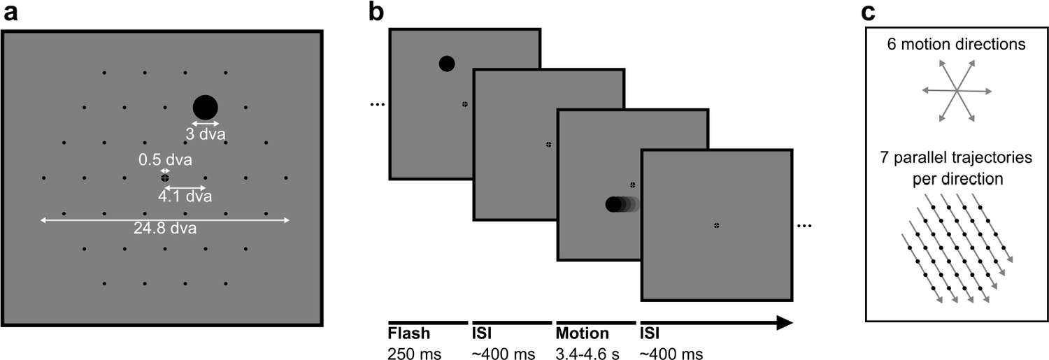
Stimuli in static and motion trials.
(a) Stimulus configuration. Stimuli were presented in a hexagonal grid. In static trials, a black circle was shown centred in 1 of the 37 positions (marked by black dots, not visible during the experiment). In motion trials, the same stimulus moved at 10.36 degrees visual angle/second (dva/s) in a straight line through the grid. A fixation point was presented in the centre of the screen and the background was 50% grey. All measurements are in dva. (b) Trial structure. A trial consisted of a black circle flashed in one position for 250 ms (static trials) or moving in a straight line for between 3350 and 4550 ms (motion trials). Trials were randomly shuffled and presented separated by an inter-stimulus interval randomly selected from a uniform distribution between 350 and 450 ms. (c) Motion trials. The moving stimulus travelled along 1 of 42 possible straight trajectories through the grid: six possible stimulus directions along the hexagonal grid axes with seven parallel trajectories for each direction. The moving stimulus passed through four to seven flash locations, depending on the eccentricity of the trajectory.
Figure 2 with 2 supplements

Classification results for decoding the position of static stimuli.
(a) Group-level pairwise classification performance of static stimulus-position discrimination sorted by distance between stimulus positions (separate lines). Classifiers were trained and tested on matched timepoints from 0 to 350 ms (i.e. the time diagonal). (b) Timepoints along the time diagonal at which likelihood of the stimulus being in the presented position (stimulus-position likelihood) is significantly above chance (n=12, p<0.05, cluster-based correction) are marked by the bar above the x-axis. The stimulus-position likelihood was significantly above chance from 58 ms onward. Shaded error bars show one standard deviation around the mean across observers. Chance level has been subtracted from all likelihoods to demonstrate the divergence from chance, in this graph and all others showing stimulus-position likelihood. (c) Stimulus-position likelihood (colour bar; Kovesi, 2015) was calculated from classification results at each combination of training and test times. Results averaged across all stimulus positions and participants are displayed as a temporal generalisation matrix (TGM). (d) Topographic maps show participant-averaged topographic activity patterns used by classifiers to distinguish stimulus positions at 141 ms post stimulus onset, the time of peak decoding (marked by an arrow in panel b). Insets in the top left of each scalp map show which two stimulus positions the classifier has been trained to discriminate. Scalp maps were obtained by combining classification weights with the relevant covariance matrix. As expected, for all four comparisons, activation was predominantly occipital and, when the stimulus positions were on either side of the vertical meridian, lateralised.
Figure 2—figure supplement 1
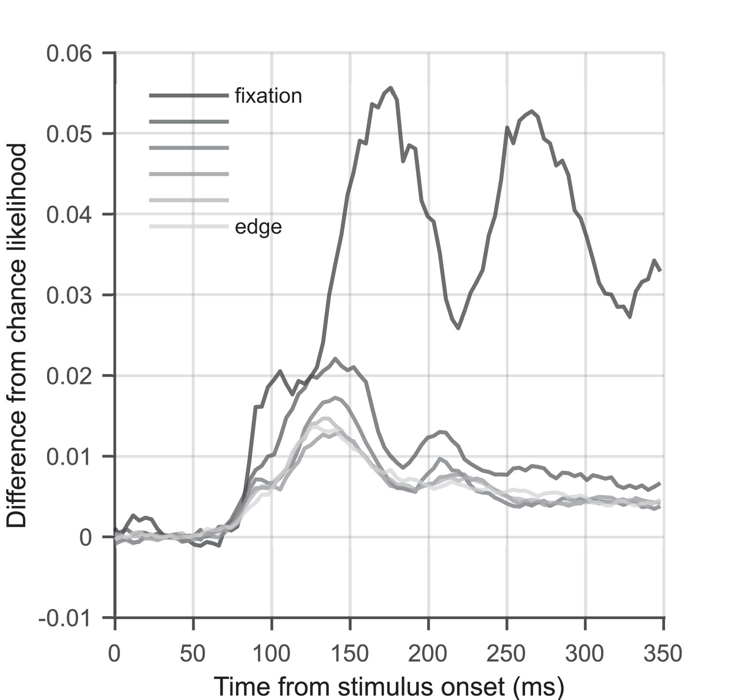
Stimulus-position likelihood as a function of eccentricity.
Graph showing the difference from chance likelihood over time, for flashed stimuli at six different eccentricities. Data were averaged over stimulus positions with the same eccentricity relative to fixation. Likelihood of the stimulus being present when presented at fixation is shown in the darkest grey; likelihood of the stimulus being present when presented at the edge of the grid (12 degrees visual angle/second [dva] from fixation) is shown in the lightest grey. Stimulus-position likelihood is higher for stimuli that are closer to fixation, with stimuli at fixation showing by far the best decoding performance. This is to be expected as a larger patch of cortex is dedicated to processing the central visual field than the periphery (Harvey and Dumoulin, 2011), and it has been shown that foveally presented stimuli elicit a much larger event-related potential than peripherally presented stimuli (Rousselet et al., 2005). It can also be observed that the relationship between likelihood and eccentricity is not as clear for stimuli located far from fixation. We believe this is because the distances between the target position and comparison positions are not uniformly distributed for central compared to peripheral stimuli. Likelihood calculations for peripheral stimuli included pairwise comparisons between stimuli that are located on opposite sides of the grid (25 dva separation), for which we obtain the best pairwise classification performance (see Figure 2a). By comparison, the target/comparison position separation is only ∼12 dva maximum for a stimulus presented at fixation. This could lead to a relative bias towards higher decoding performance for peripheral compared to central locations.
Figure 2—figure supplement 2
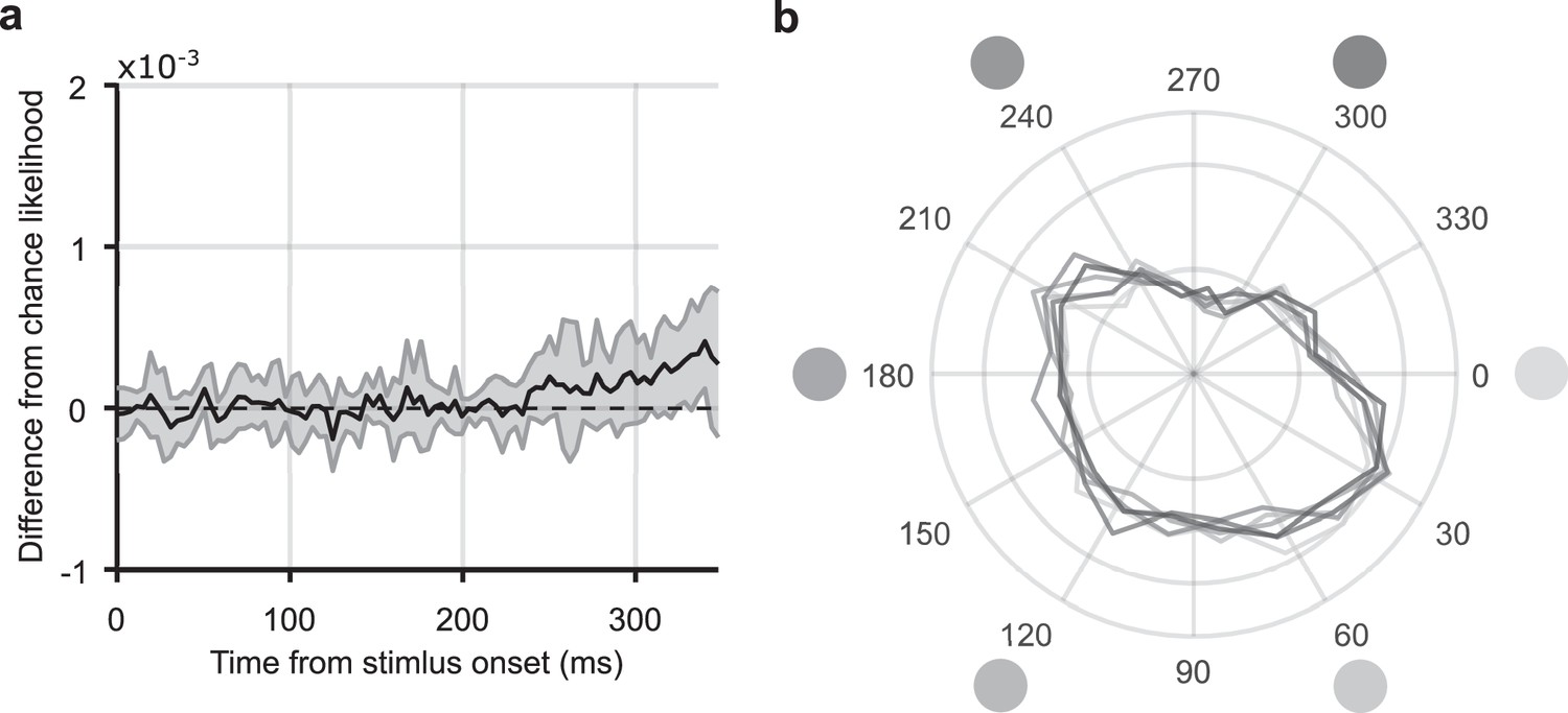
Analysis of eye movements.
(a) The same decoding analysis that was applied to the EEG response to the static stimuli was applied to the x-y position of the eyes (measured using concurrent eyetracking). The graph shows mean stimulus-position likelihood at each timepoint from stimulus onset. Error bars show one standard deviation around the mean across observers. Stimulus-position likelihood was not significantly above chance at any timepoint between 0 and 350 ms (n=12, p>0.05, cluster-based correction). (b) Distribution of eye angles (density plot) following presentation of stimuli in the six outermost stimulus positions, 12.4 degrees visual angle/second (dva) from fixation. The angle of the stimulus around fixation is marked by the greyscale circles; corresponding coloured lines show the distribution of eye angle for that stimulus. For each trial and each participant, the average eye angle between 50 and 350 ms was included. It can be observed that the distribution of eye angle does not change depending on the angular position of the stimulus. This observation was confirmed with a multi-sample test for equal median distributions (Berens, 2009), which showed that the median eye angle, averaged from 50 to 350 ms post flash onset, was not significantly different for any of the outermost corner stimulus position: P(11) = 2.00, p = 0.849. Both these analyses suggest that participants’ eye positions did not systematically vary according to the stimulus location.
Figure 3 with 1 supplement
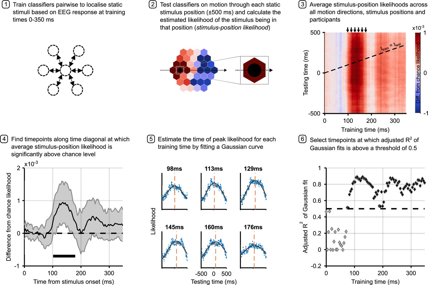
Analysis pipeline for motion trials.
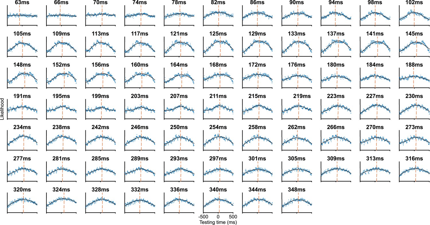
Panels describe steps in calculating the time to peak stimulus-position likelihood in motion trials, including graphs of relevant data for each step. Steps 1 and 2 describe the classification analysis applied to obtain the stimulus-position likelihoods. The figure in step 3 shows the group-level temporal generalisation matrix for training on static stimuli and testing on moving stimuli. The black dotted line shows the ‘diagonal’ timepoints, where the time elapsed since the moving stimulus was at the flash position equals the training time. Step 4 shows timepoints along this diagonal at which the stimulus-position likelihood was significantly above chance, as established through permutation testing. Significance is marked by the solid black line above the x-axis; the likelihood is significantly above chance from 102 to 180 ms (n=12, p<0.05, cluster-based correction). Shaded error bars show one standard deviation around the mean. The figure in step 5 shows the same data as step 3 for selected training times (arrows above temporal generalisation matrix [TGM] correspond to subplot titles). Each subplot shows a vertical slice of the TGM. Blue points show data, to which we fit a Gaussian curve (black lines) to estimate the time of peak likelihood for each training time (dashed orange lines). These are the data points plotted in Figure 4a and b. Step 6 shows adjusted R2 of Gaussian fits for each training timepoint. A cutoff of 0.5 was used to select timepoints at which the Gaussian fit meaningfully explains the pattern of data.
Figure 3—figure supplement 1
Fitted Gaussian curves at extended training times.
Each subplot shows a vertical slice of the temporal generalisation matrix (TGM) in Figure 3, step 3. Blue points show data, to which we fit a Gaussian curve (black lines) to estimate the time of peak likelihood for each training time (dashed orange lines).
Figure 4

Neural response latency during motion processing.
(a) Latencies of the peak stimulus-position likelihood values during motion processing. The timepoint at which peak likelihood was reached is plotted against training time. Error bars around points show bootstrapped 95% confidence intervals of the peak shift parameter of the Gaussian fit, computed from n = 12 participants (see Figure 3, step 5). It can be observed that the peak time increases and decreases, then levels out. Points of inflection within this timeseries were identified using piecewise regression (shown in black). The number of inflection points, or knots, was established by comparing the R2 of piecewise regression fits, as shown in the inset graph. It was determined that six knots was optimal; positions of these knots are marked by grey dotted lines on the main graph. (b) Time to peak likelihood during the initial feedforward sweep of activity through the visual cortex. Displayed is a subset of points from those shown in panel a, corresponding to a restricted time-window between the first two knots, during which the first feedforward sweep of activity was most likely occurring. The dotted diagonal shows the 45° line, where the time of peak likelihood would equal the training time. Data points from static trials (green) should theoretically lie along this line, as, in this case, the training and test data were subsets of the same trials. Straight lines were fit separately for static (F(21,19) = 805.45, p=1.24 × 10⁻¹⁷) and motion trials (F(21,19) = 40.91, p=3.07 × 10⁻⁶). Both lines had similar gradients, close to unity, indicating equivalent cumulative processing delays for static and motion trials within this training time-window. However, the intercept for motion was much earlier at –80 ms. The mean distance between the two lines is marked, indicating that position representations were activated ∼70 ms earlier in response to a moving stimulus compared to a flashed one in the same location. Time to peak likelihood at the beginning of the feedforward sweep was approximately 0 ms, indicating near-perfect temporal alignment with the physical position of the stimulus. (c) Illustration of compensation for neural delays at different cortical processing levels. The static stimulus (green, top) and the moving stimulus (orange, bottom) are in the same position at time = 0 ms (black dashed line), but there is a 73 ms latency advantage for the neural representations of the stimulus in this position when it is moving. Each separate curve represents neural responses emerging at different times during stimulus processing, where higher contrast corresponds to early visual representations and lower contrast corresponds to later visual representations. The earliest neural response, likely originating in early visual cortex, represents the moving stimulus in its real-time location. The consequence of this is a shift in the spatial encoding of the moving stimulus: by the time neural representations of the flash emerge, the moving stimulus will be represented in a new location further along its motion trajectory. The relative distance between the subsequent curves is the same for moving and static stimuli, because there is no further compensation for delays during subsequent cortical processing.
Author response image 1
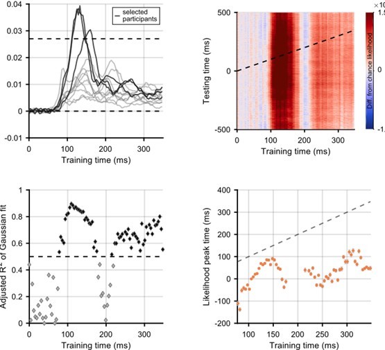
Selection of participants for whom flash decoding is best.
Participants were selected if the difference from chance stimulus-position likelihood (averaged across all stimulus positions) was above a threshold of 1/37 (which is the same as the likelihood being twice as high as chance level). The top left panel shows the difference from chance likelihood against training time. The three selected participants are shown in a darker colour. The remaining panels show graphs corresponding to the graphs in the main manuscript: the analysis is exactly the same.
Author response image 2
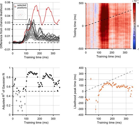
Selection of positions for which flash decoding is best.
Positions were selected if the difference from chance stimulus-position likelihood (averaged across all participants) was above a threshold of 1/37. In the top left panel, lines show difference from chance likelihood for all of the 37 possible stimulus locations. Inset on the top left panel shows the selected positions, highlighted in red (fixation) and black on the graph. Everything else is the same as above.
Additional files
Download links
A two-part list of links to download the article, or parts of the article, in various formats.
Downloads (link to download the article as PDF)
Open citations (links to open the citations from this article in various online reference manager services)
Cite this article (links to download the citations from this article in formats compatible with various reference manager tools)
Position representations of moving objects align with real-time position in the early visual response
eLife 12:e82424.
https://doi.org/10.7554/eLife.82424


