Visual and motor signatures of locomotion dynamically shape a population code for feature detection in Drosophila
- Department of Neurobiology, Stanford University, United States
Figures
Figure 1
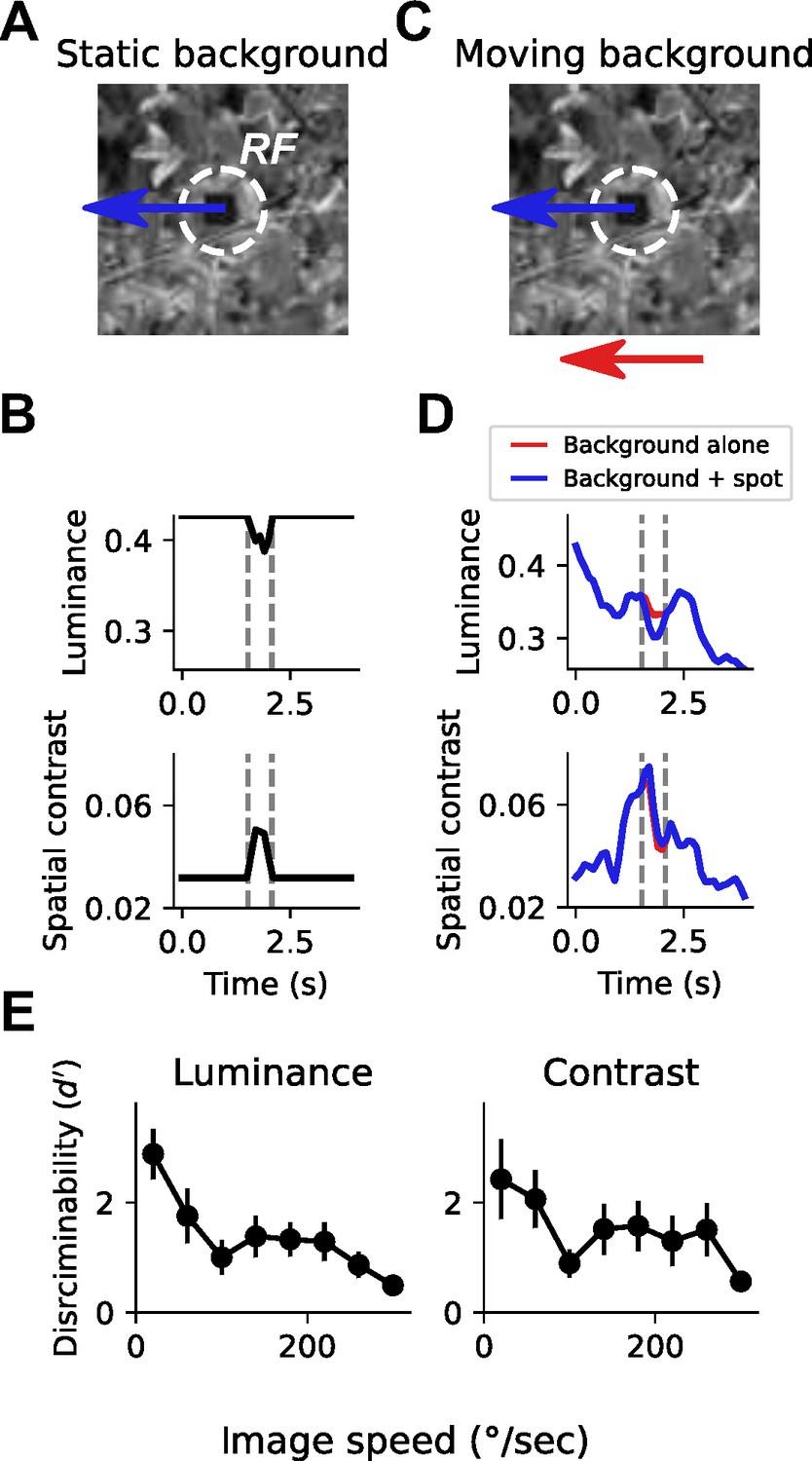
Small spot detection is unreliable during self-generated rotation.
(A) Schematic illustrating the stimulus and detection task. A small dark spot on top of a grayscale natural image moved through a visual receptive field (white dashed circle). (B) When the background image was stationary, small spot detection was trivial using either local luminance (top) or spatial contrast (bottom) cues. Vertical dashed lines indicate the window of time that the spot passes through the receptive field. (C) To mimic an object detection task during self-generated rotation, we moved the background image independently of the spot with a variable speed. (D) Movement of the background image alone (red trace) caused dramatic fluctuations in luminance and contrast within the receptive field. The addition of the small moving spot (blue trace) caused relatively small changes in the luminance or contrast signal, which depends on the spatial structure of the image. (E) Discriminability of the spot based on luminance (left) or contrast (right) during the time period when the spot passed through the receptive field, as a function of background image speed. Points indicate mean ± S.E.M. across a collection of 20 grayscale natural images. Even for slow background speeds, detection was corrupted, and the discriminability of the spot decreased further as the background speed increased.
Figure 2 with 1 supplement

A method to extract optic glomerulus population responses from bulk-labeled neuropil.
(A) Schematic of the left half of the brain showing optic lobe and the optic glomeruli of the central brain, which receive inputs from distinct visual projection neurons. Me: Medulla, LP: Lobula Plate, Lo: Lobula, PVLP: Posterior Ventrolateral Protocerebrum, PLP: Posterior Lateral Protocerebrum. (B) Schematic of imaging and stimulation setup. (C) LC4 neurons expressing plasma membrane-bound myr::tdTomato (magenta) and presynaptically localized syt1GCaMP6f (green), which is enriched in axons in the optic glomerulus. (D) For pan-glomerulus imaging, cholinergic neurons express myr::tdTomato (purple) and syt1GCaMP6f (green). The optic glomeruli in the PVLP/PLP can be seen. (E) Pipeline for generating the mean brain from in vivo, high-resolution anatomical scans and aligning this mean brain to the JRC2018 template brain. Using this bridging registration, neuron and presynaptic site locations from the hemibrain connectome can be transformed into the mean brain space, allowing in vivo voxels to be assigned to distinct, non-overlapping optic glomeruli. (F) Montage showing z planes (rows) of the registered brain space for the mean brain myr::tdTomato (purple) and syt1GCaMP6f (green) channels (first and second columns, respectively), JRC2018 template brain (third column) and optic glomeruli map (fourth column). (G) Mean brain images at indicated z levels showing distinct glomerulus locations of interest. (H) For the locations of interest in (G), the optic glomerulus map is overlaid on the mean brain (first column) and alignment is shown for each of the 10 individual flies (remaining columns). For all images, scale bar is 25 μm.
Figure 2—figure supplement 1
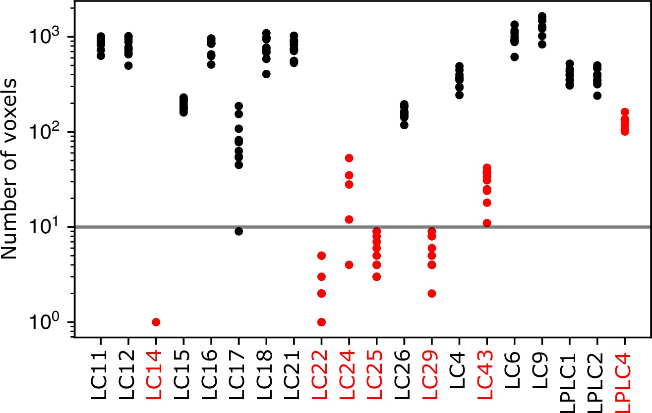
Number of voxels in each LC/LPLC glomerulus.
For each LC/LPLC glomerulus in or near the imaging volume, the number of voxels in each transformed glomerulus mask that lies within the imaging volume is shown for 10 flies. Glomeruli highlighted in red were excluded from this analysis because they were consistently small, or often not included in the volume. The LPLC4 glomerulus was excluded because this glomerulus is co-extensive with the LC22 glomerulus. The horizontal line indicates a threshold we set for further excluding glomeruli from individual flies for being small in that fly’s imaging volume. For example, the LC17 glomerulus was sometimes excluded from individual flies because it lies at the bottom of our imaging volume, and brain motion or slight changes in the imaging depth caused the imaged portion of the LC17 glomerulus to be very small.
Figure 3
Pan-glomerulus imaging reliably measures optic glomerulus responses dominated by visual projection neurons.
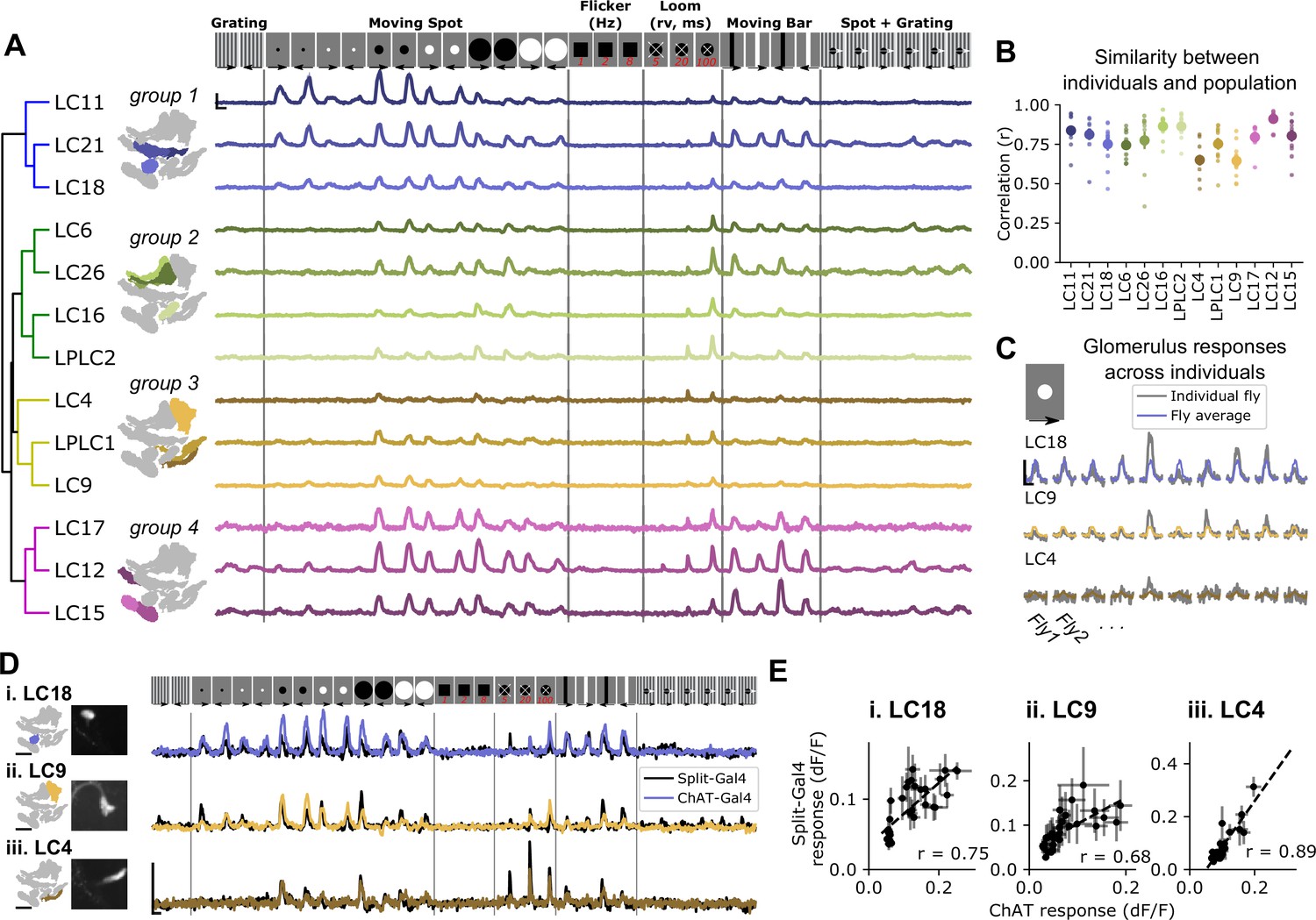
(A) Responses of thirteen optic glomeruli to a panel of synthetic visual stimuli (top, see Materials and methods). Responses are shown according to the indicated stimulus order, but stimuli were presented in randomly interleaved trial order. Shown are mean glomerulus response traces across 10 flies, shading indicates S.E.M. We hierarchically clustered mean glomerulus responses to yield four functional groups of glomeruli. (B) Visual tuning can be reliably estimated in single flies using pan-glomerulus imaging. For each glomerulus, we computed the correlation between each individual fly tuning and the mean tuning (excluding that fly). Large dots and bars indicate mean ± S.E.M., and small dots correspond to individual flies. (C) Example responses of three glomeruli in individual flies to a 15° bright moving spot. For each panel, the colored trace is the across-fly average response and the gray trace is the individual fly response. (D) Comparison of glomerulus tuning to the LC neurons that dominate their input, for three glomerulus/LC pairs. Left: glomerulus map and example image of the LC axons. Right: syt1GCaMP6f responses to the stimulus panel above. Colored traces show tuning measured using pan-glomerulus imaging procedure and black traces show split-Gal4 LC responses. (E) For the three LC types in (D), the tuning of LC axons is highly correlated with the tuning of corresponding optic glomeruli (pan-glomerulus imaging: n=10 flies; Split-Gal4 imaging: n=5, 6, and 4 flies for LC18, LC9, and LC4, respectively). For all calcium traces, Scale bar is 2 s and 25% dF/F. r is the Pearson correlation coefficient.
Figure 4 with 3 supplements
Glomerulus responses are modulated by a shared gain factor that impacts stimulus encoding fidelity.
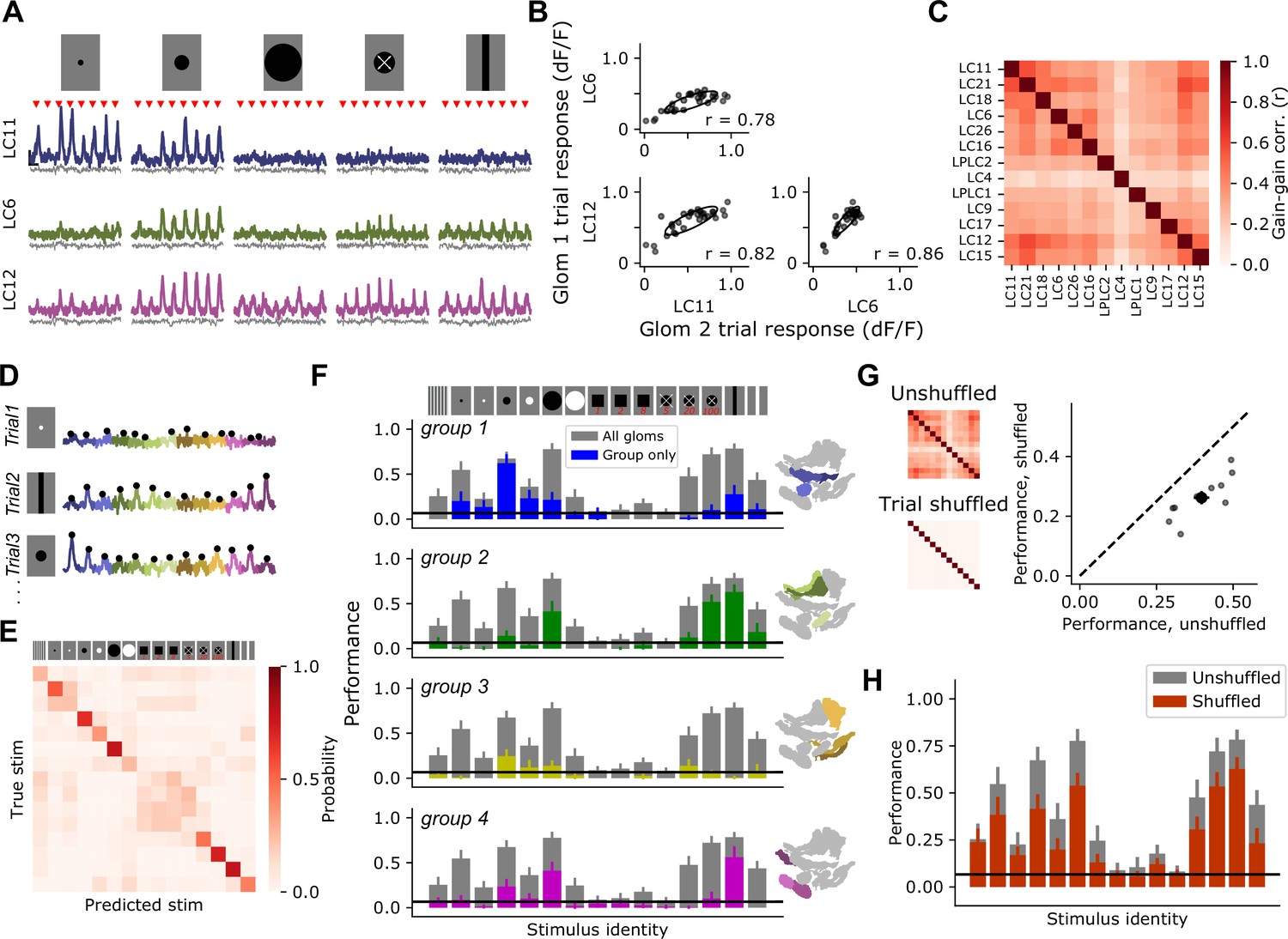
(A) For a reduced stimulus set (images above), we presented many trials in a randomly interleaved order. For display, we have grouped responses by stimulus identity. Red marks indicate stimulus presentation times. Example single-trial responses for representative glomeruli show large trial-to-trial variability. Scale bar is 4 s and 25% dF/F. Gray traces below show simultaneous glomerulus signals from the red (myr::tdTomato) channel showing that fluorescence changes are due to visually driven responses, not motion artifacts or other imaging factors. (B) For the example glomeruli in (A), plotting one glomerulus response amplitude against another for a given stimulus (here, a 15° moving spot), reveals high correlated variability. Each point is a trial. Ellipses show 2D Gaussian fit derived from the trial covariance matrix. r is the Pearson correlation coefficient. (C) Trial-to-trial variability is strongly correlated across different glomeruli. Heatmap shows the average correlation matrix across all stimuli and flies (n=17 flies). (D) Single-trial responses of 13 optic glomeruli, concatenated together for each trial. Stimulus identity is indicated to the left. Black dots indicate the peak responses of each glomerulus on each trial, which will be used for stimulus decoding. The response amplitudes for all 13 glomeruli were used to train a multinomial logistic regression model to predict stimulus identity (see Materials and methods). (E) Confusion matrix, with rows and columns corresponding to stimulus identity above. (F) We used held-out data to test the ability of the decoding model to predict the stimulus identity given the single-trial response amplitudes of different groupings of glomeruli. In each barchart, gray bars correspond to a model with access to all 13 glomerulus responses for each trial. Colored bars show mean ± S.E.M. performance of a model with access to only the indicated functional group of glomeruli. (G) Trial shuffling population responses remove pairwise correlations among glomeruli (insets to the left show correlation matrices before and after trial shuffling). Right: Decoding model performance, averaged across all stimuli, for each fly (n=11 flies). Large marker shows mean ± S.E.M. (H) Performance of the decoding model suffers across all stimulus classes when trial-to-trial correlations are removed.
Figure 4—figure supplement 1
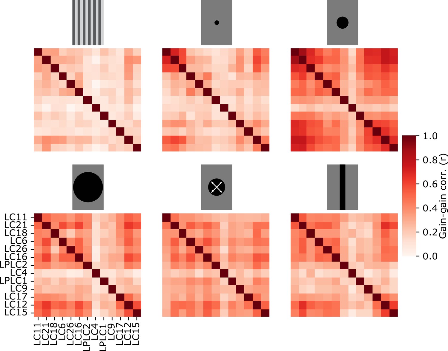
Trial correlation matrix for each stimulus class.
From the trial covariance analysis in Figure 4, each panel shows the trial correlation matrix for each of the six stimuli shown in the reduced stimulus set for these experiments. Positive correlations are seen for all stimuli, but tend to be higher for stimuli that drive glomerulus responses strongly.
Figure 4—figure supplement 2
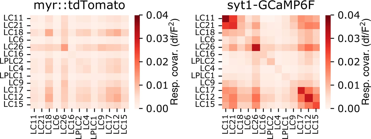
Trial covariance matrix for both myr::tdTomato and sytGCaMP6f fluorescence channels.
Trial covariance matrix for both the red (myr::tdTomato) and green (syt1GCaMP6f) fluorescence signals, averaged across flies (n=18 flies), showing that trial covariance in the green channel is dominated by neural responses, not by brain movement or other factors associated with imaging. Residual covariance structure in the red channel is present primarily for glomeruli with weak visually driven responses.
Figure 4—figure supplement 3
Decoding stimulus identity for a reduced subset of behaviorally discriminable stimulus classes.
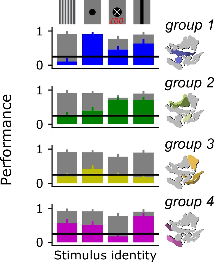
We performed our decoding analysis on a reduced subset of visual stimulus classes that are known to drive distinct behaviors in flies: a drifting grating, a dark spot, a looming spot, and a vertically oriented bar. Gray bars show model performance with access to all optic glomeruli, colored bars show model performance using only responses from the indicated glomerulus group. Horizontal line shows 25% chance level.
Figure 5 with 3 supplements
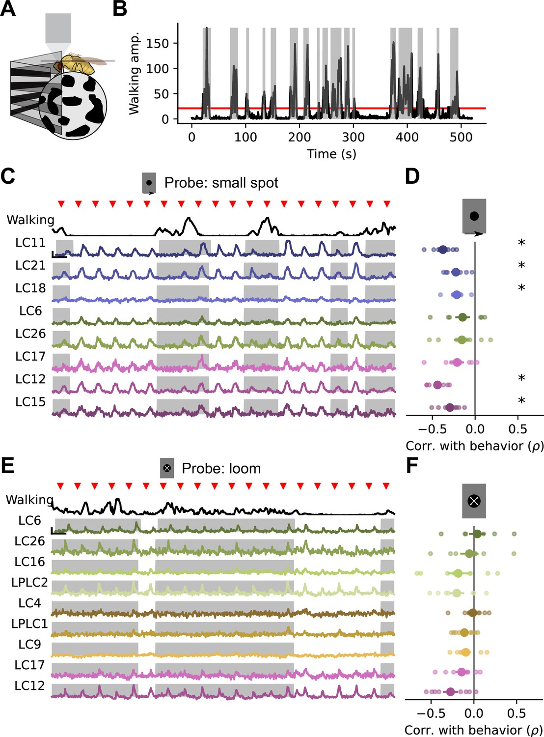
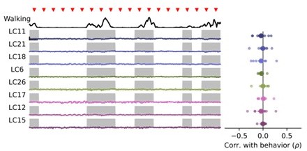
Walking behavior suppresses glomerulus responses to small object stimuli.
(A) Schematic showing fly on air-suspended ball for tracking behavior. (B) We used the change in ball rotation to measure overall walking behavior. Red line indicates threshold for binary classification of behaving versus nonbehaving, and gray shading indicates trials that were classified as behaving. (C) We presented a 15° moving spot repeatedly to probe glomerulus gain throughout the experiment. Example responses and quantification are shown only for glomeruli which respond reliably to this probe stimulus. Red triangles show stimulus presentation times. Black traces (top) show walking amplitude, and gray shading indicates trials classified as behaving. Scale bar is 4 sec and 25% dF/F. (D) Correlation (Spearman’s rho) between behavior and response amplitude. Each small point is a fly, large point is the across-fly mean (n=8 flies), and asterisks indicate glomeruli with a significant negative correlation between response gain and behavior (One sample t-test, p<0.05 after correction for multiple comparisons). (E–F) Same as C-D for a looming probe stimulus, with responses from the subset of glomeruli that respond strongly to looming stimuli. On average, there is no correlation between behavior and loom response strength (n=8 flies).
Figure 5—figure supplement 1
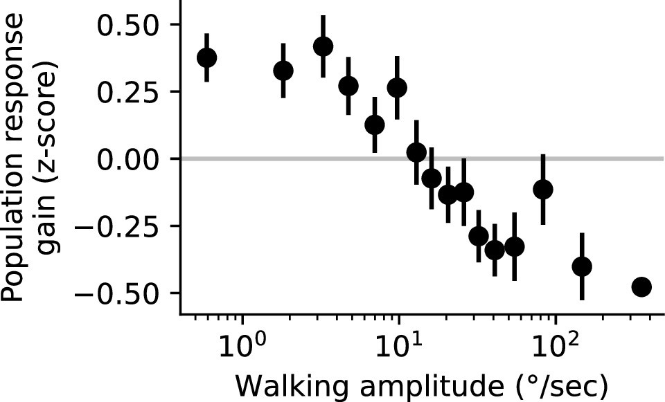
Population response gain as a function of walking amplitude.
Population response gain was defined as the z-scored trial response amplitude, averaged across all glomeruli that showed a significant negative correlation with behavior in Figure 5. We binned this population gain measure by peak walking amplitude on that trial (into equally-populated bins), to examine the relationship between peak walking amplitude and population response gain. Horizontal line at zero indicates the average response gain across all trials (n=8 flies).
Figure 5—figure supplement 2
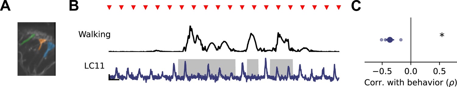
Genetically targeted VPN imaging shows behavioral modulation of response gain.
(A) Image of LC11 dendrites in Lobula, with three dendritic stalk ROIs highlighted. (B) Example walking amplitude (top, black) and LC11 response (bottom, blue) to repeated presentations of a small moving spot, as in Figure 5. (C) Spearman correlation between response gain and walking amplitude (n=4 flies). Asterisk indicates p<0.05 (one sample t-test).
Figure 5—figure supplement 3
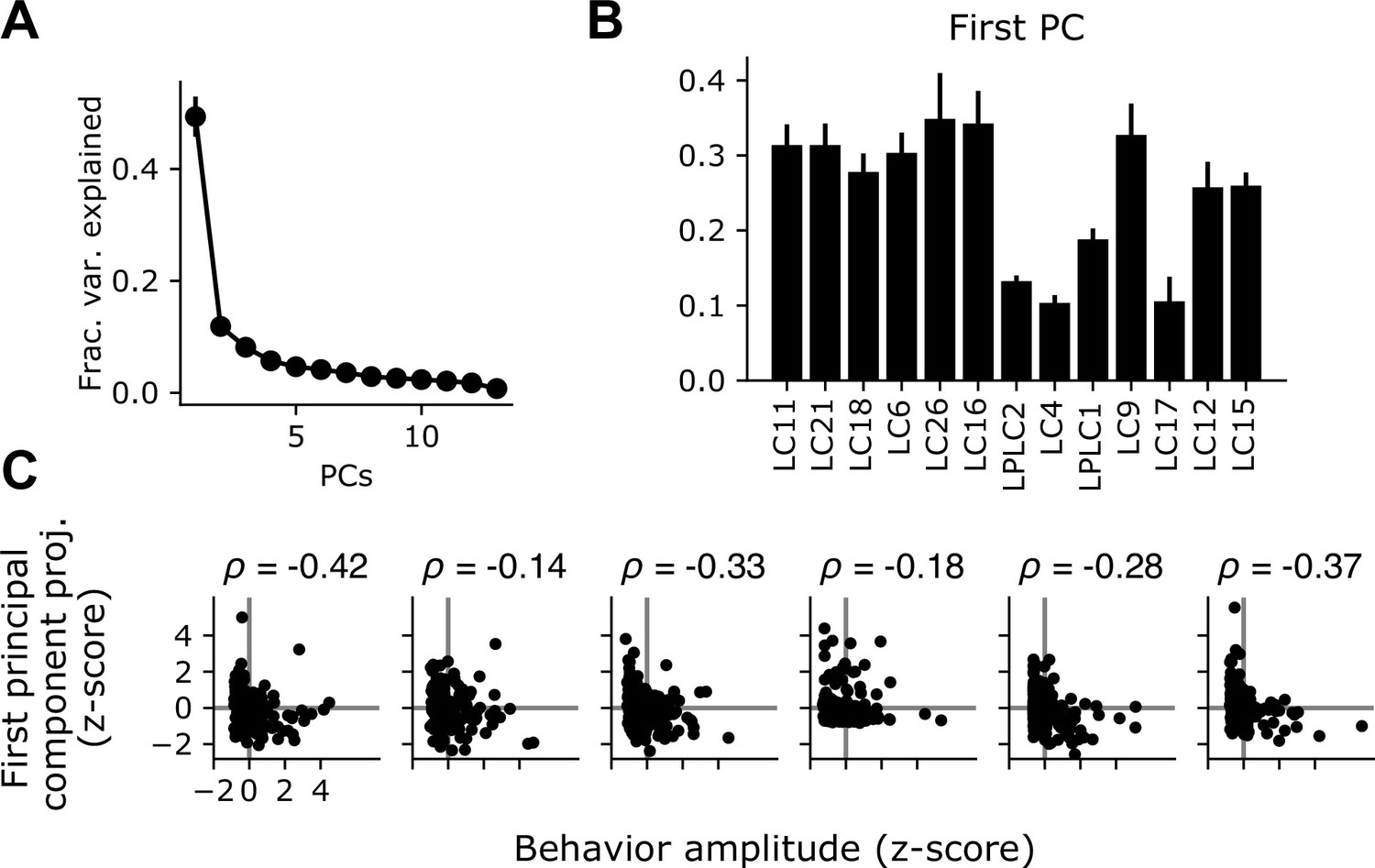
The shared glomerulus gain factor is negatively correlated with behavior.
(A) Eigenvector decomposition of the covariance matrix reveals a dominant principal component which accounts for a large plurality of the trial-to-trial variance across the population. Points show mean +/- S.E.M. across flies (n=6 flies). (B) The first principal component of the response gain, averaged across flies. (C) For the variance analysis experiments in Figure 4, we tracked behavior for a subset of the animals tested. For each fly, we z-scored the behavior amplitude across trials as well as the shared gain factor for each trial (equal to the projection of the first PC against the population response matrix). Each plot shows the relationship between the trial-by-trial shared gain factor and the average behavior amplitude for each trial. For every fly, there was a negative correlation between these two measures (mean = –0.23, n=6 flies).
Figure 6
Visual input associated with rotational motion suppresses optic glomerulus responses.
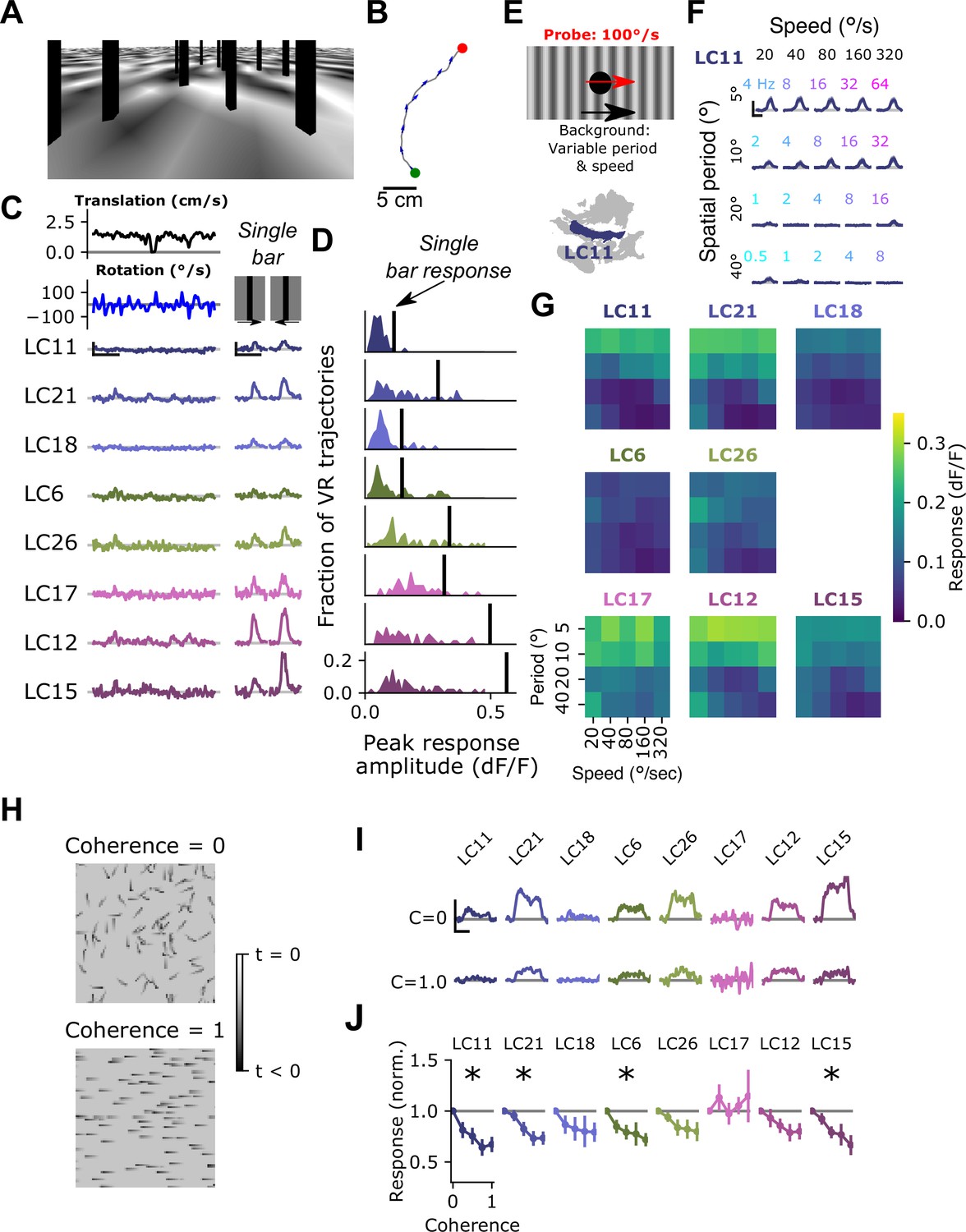
(A) Still image from a VR stimulus. (B) Twenty second snippet of a fly walking trajectory. Green and red points indicate start and end of the trajectory, respectively. Arrows show the fly’s heading. (C) For an example fly, responses of small object detecting glomeruli to an example virtual reality trajectory. These glomeruli respond very weakly to the virtual reality stimulus, despite showing strong, reliable responses to solitary vertical bars (right) similar to those present in the virtual reality scene. Scale bar is 5 s and 25% dF/F. (D) Histograms showing, for each glomerulus, the distribution of peak responses to each VR trajectory. Vertical line indicates mean response to a single dark, vertical bar stimulus (five VR trajectories were presented to each fly, n=10 flies). (E) Schematic showing the surround suppression tuning stimulus. A small dark probe stimulus moves through the center of the screen while a grating with varying spatial frequency and speed moves in the background. (F) For the LC11 glomerulus, probe responses are suppressed by low spatial frequency gratings across a range of speeds consistent with locomotor turns. Small, color-coded numbers indicate the temporal frequency associated with each grating speed and spatial period. Scale bar is 2 s and 25% dF/F. (G) Heatmaps showing probe responses as a joint function of background spatial period and speed for each of these 8 glomeruli (n=10 flies). (H) Schematic of random dot coherence stimulus. At zero coherence (top image), each dot moves independently of all the other dots. At a coherence of 1.0 (bottom image), all dots move in the same direction. (I) For an example fly, responses of the small object detecting glomeruli are shown to coherence values of 0 (top row) and 1.0 (bottom row). Scale bar is 2 s and 25% dF/F. (J) Summary data showing response amplitude (normalized to the 0 coherence condition within each fly) of each glomerulus to varying degrees of motion coherence. Asterisk at the top indicates a significant difference between the response to 0 and 1 coherence (n=11 flies, paired t-test, p<0.05 after correction for multiple comparisons).
Figure 7
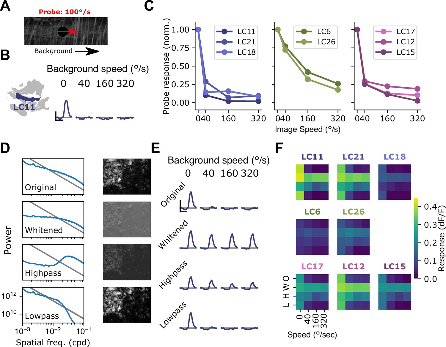
Visual suppression is tuned to natural image statistics.
(A) Stimulus schematic: a small spot probe is swept across the visual field while a grayscale natural image moves in the background at a variable speed. (B) For the LC11 glomerulus, natural image movement strongly suppresses the probe response across a range of speeds (average across three images, n=8 flies). (C) Mean probe response as a function of background image speed, normalized by probe response with static background. Surround speed tuning curves are grouped by functional glomerulus groupings for the small object detecting glomeruli. (D) Average power spectra (left) and example image (right) for the original natural images (top), whitened images (second row), high-pass filtered images (third row), and low-pass filtered images (bottom row). Gray line shows p . (E) For LC11, image suppression of probe responses is attenuated by whitening the image or high-pass filtering it, but not by low-pass filtering the image. (F) Dependence of probe suppression on image speed and filtering for each of the eight small object detecting glomeruli (n=9 flies). Scale bar is 2 s and 25% dF/F.
Figure 8

Natural fly walking is punctuated by saccadic turns.
(A) Example unconstrained fly walking trajectory measured in an open behavioral arena. Arrows show the fly’s heading. Green point indicates start of walking trajectory. Scale bar=1 cm. (B) Heatmap of instantaneous forward velocity and rotational speed across all time points from 81 fly trajectories. Note logarithmic color scale. (C) Example trace of instantaneous angular velocity (top) and instantaneous forward velocity (bottom). Red arrowheads on top indicate saccades. (D) Histogram of inter-turn intervals shows a peak around 1 s and a long tail. (E) Histogram of angular speed (top) and forward velocity (bottom) within a 400 ms window around a saccade (red) or during the intersaccade interval (gray).
Figure 9
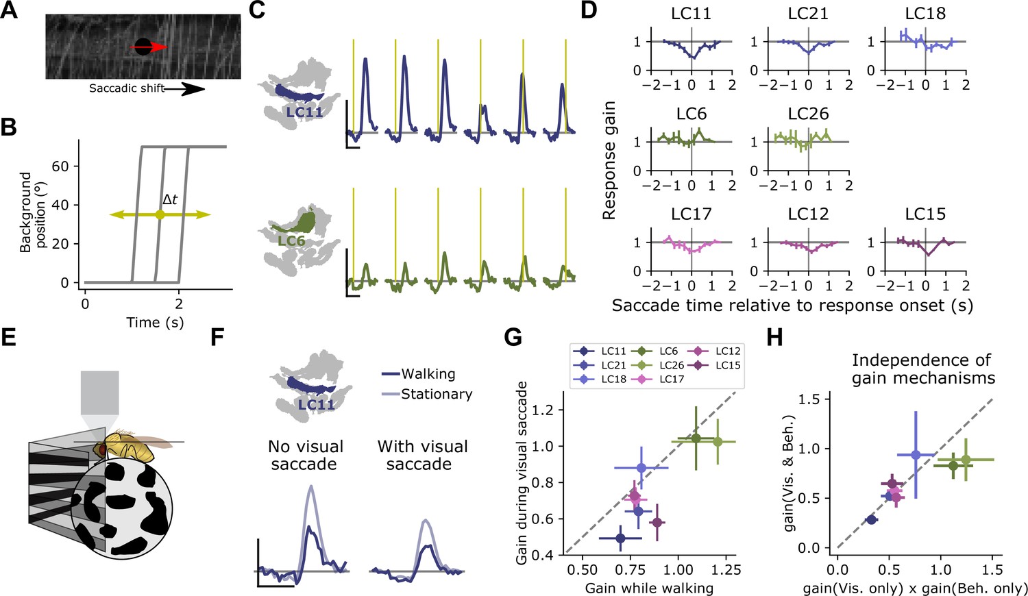
Visually driven saccade suppression works in concert with behavioral suppression.
(A) Stimulus schematic: A small moving probe is used to measure glomerulus response gain while a full-field natural image in the background undergoes a fast, ballistic lateral displacement meant to mimic fly walking saccades. (B) The time of the saccade is varied throughout the trial, such that it occurs at different phases of the probe response. Each saccade lasted 200 ms and translated the image by 70°. (C) Trial-average probe responses in an example LC11 glomerulus (top) and an example LC6 glomerulus (bottom). Saccade times are indicated by the yellow vertical line in each panel. As the saccade approaches the probe in time, the probe response is suppressed in LC11 but not LC6. (D) Summary data showing, for each small object detecting glomerulus, the response gain as a function of saccade time relative to the response onset. t=0 corresponds to coincident probe response and saccade onset. Suppression is strongest when the saccade occurs near probe response onset (n=5 flies). (E) We monitored fly walking behavior while presenting the saccadic visual stimuli above. (F) For an example LC11 glomerulus, both the saccadic stimulus and walking behavior reduced probe responses, and these gain control mechanisms could be recruited separately. (G) Population data showing average response gain for visual saccades versus response gain during walking behavior, for each small object detecting glomerulus. Most glomeruli lie below unity (dashed line), indicating that visual saccade suppression is typically stronger than behavior-linked suppression. These two sources of suppression are also correlated across glomeruli (r=0.80, Pearson correlation coefficient). (H) For each small object detecting glomerulus, we compared the response gain when both visual-related and motor-related gain modulation were recruited (vertical axis) to the product of both response gains in isolation (horizontal axis). Dashed line is unity, and points falling along that line indicate a linear interaction between those forms of gain control.
Author response image 1
Additional files
Download links
A two-part list of links to download the article, or parts of the article, in various formats.
Downloads (link to download the article as PDF)
Open citations (links to open the citations from this article in various online reference manager services)
Cite this article (links to download the citations from this article in formats compatible with various reference manager tools)
Visual and motor signatures of locomotion dynamically shape a population code for feature detection in Drosophila
eLife 11:e82587.
https://doi.org/10.7554/eLife.82587


