A tug of war between filament treadmilling and myosin induced contractility generates actin rings
- Department of Chemical and Biomolecular Engineering, University of Maryland, College Park, United States
- Department of Physics, University of Maryland, College Park, United States
- Biological Sciences Graduate Program, University of Maryland, College Park, United States
- Biophysics Graduate Program, University of Maryland, College Park, United States
- Institute for Physical Science and Technology, University of Maryland, United States
- Department of Chemistry and Biochemistry, University of Maryland, United States
Figures
Figure 1 with 3 supplements

Actin and NMII distribution within actin rings in T cells and simulation.
(a–b) Representative snapshots of actin (a) and NMII (b) in actin rings of live Jurkat T cells activated on anti-CD3 antibody-coated coverslips. Actin is labeled by tdTomato F-tractin (magenta), and NMII is labeled by MLC-EGFP (green). (c) Merged fluorescence image (left panel) showing distribution of actin and NMII within the T cell actin ring. Inner and outer regions of the ring are indicated. Normalized fluorescence intensity profiles of F-actin and NMII (right) along the dashed line shown in the left panel. (a–c) Scale bar = 10 µm. (d) Setup of simulations using MEDYAN with the major cytoskeletal components labeled. (e) A representative snapshot of the simulation (left)and the corresponding distribution of actin and NMII along the diameter of the ring (right). . Scale bar = 1µm.
Figure 1—figure supplement 1
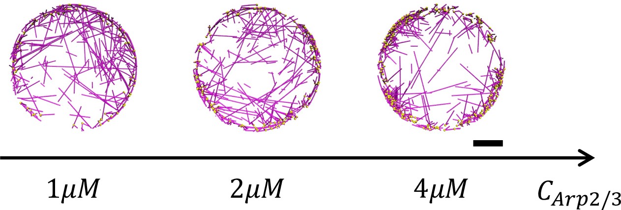
Representative snapshots of actin networks that consist of 40µM actin and 1–4µM Arp2/3 without crosslinkers or motors.
Arp2/3 (represented as yellow beads) is activated 500nm away from the boundary. Scale bar = 1 µm.
Figure 1—figure supplement 2
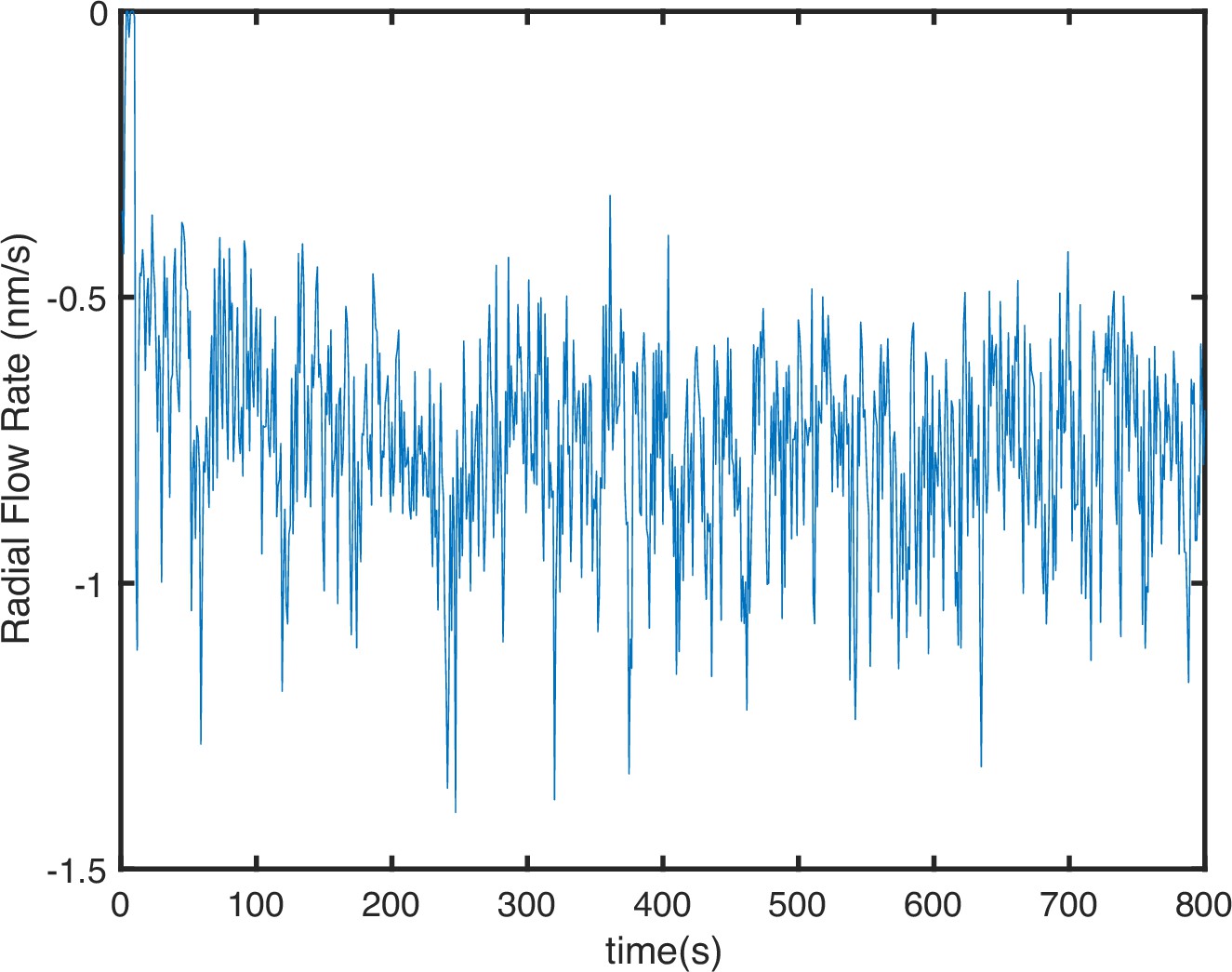
F-actin flow rate along the radial direction.
Flow rate is quantified by tracking the mean displacement of individual F-actin molecules. Negative flow rate indicates centripetal motion.
Figure 1—video 1
Timelapse movie of F-actin and NMII in Jurkat T cells activated by anti-CD3 coated stimulatory coverslips as shown in Figure 1a.
F-actin is labeled by tdTomato-F-tractin, and NMII is labeled by MLC-EGFP. Scale bar is 10µm. Timestamp indicates time since seeding cells.
Figure 2 with 10 supplements
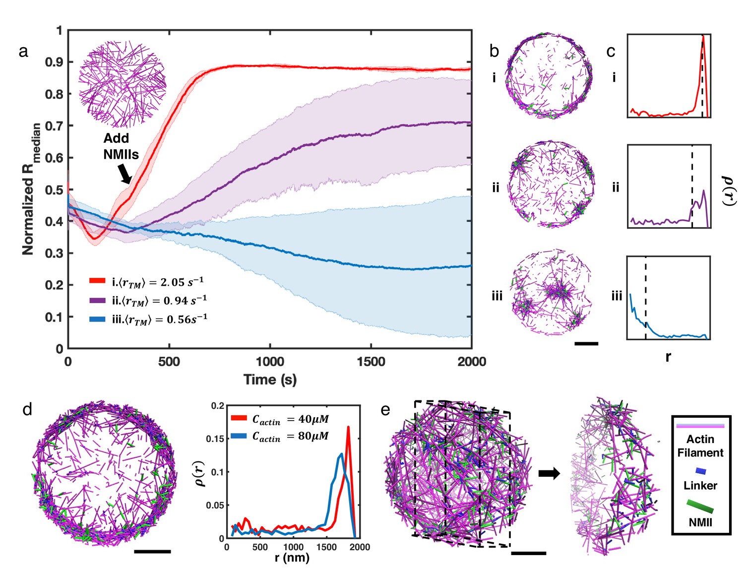
NMII contractility induces geometric collapse of treadmilling actin filaments.
(a) Normalized medians of radial filament density distribution () at different treadmilling rates () are shown. The treadmilling rate is defined as the average number of actin monomers added per filament per second at the barbed ends - equivalent to the rate of F-actin depletion from the pointed ends - after reaching the kinetic steady state (See Simulation Methods and Figure 2—figure supplement 7 for details). 0.06µM of NMII and 4µM of alpha-actinin were added at 301s. The inset figure is a snapshot at t=300s of networks with . The shaded error bars represent the standard deviation across 5 runs. (b–c) Representative snapshots at each treadmilling condition (b) and their radial filament density distribution, (c) are shown. Dashed lines in (c) indicate the position of . (d) Representative snapshot of ring-like networks with 80µM actin (left), and of actin rings with 40µM actin and 80µM actin (right) are shown ( 1.35 s–1). (e) A snapshot of a spherical cortex-like network (left) and a slice showing the internal structure (right). (a,b,d,e) Actin filaments are magenta cylinders, NMIIs are green cylinders and linkers are blue cylinders in all snapshots. All scale bars are 1µm.
Figure 2—figure supplement 1
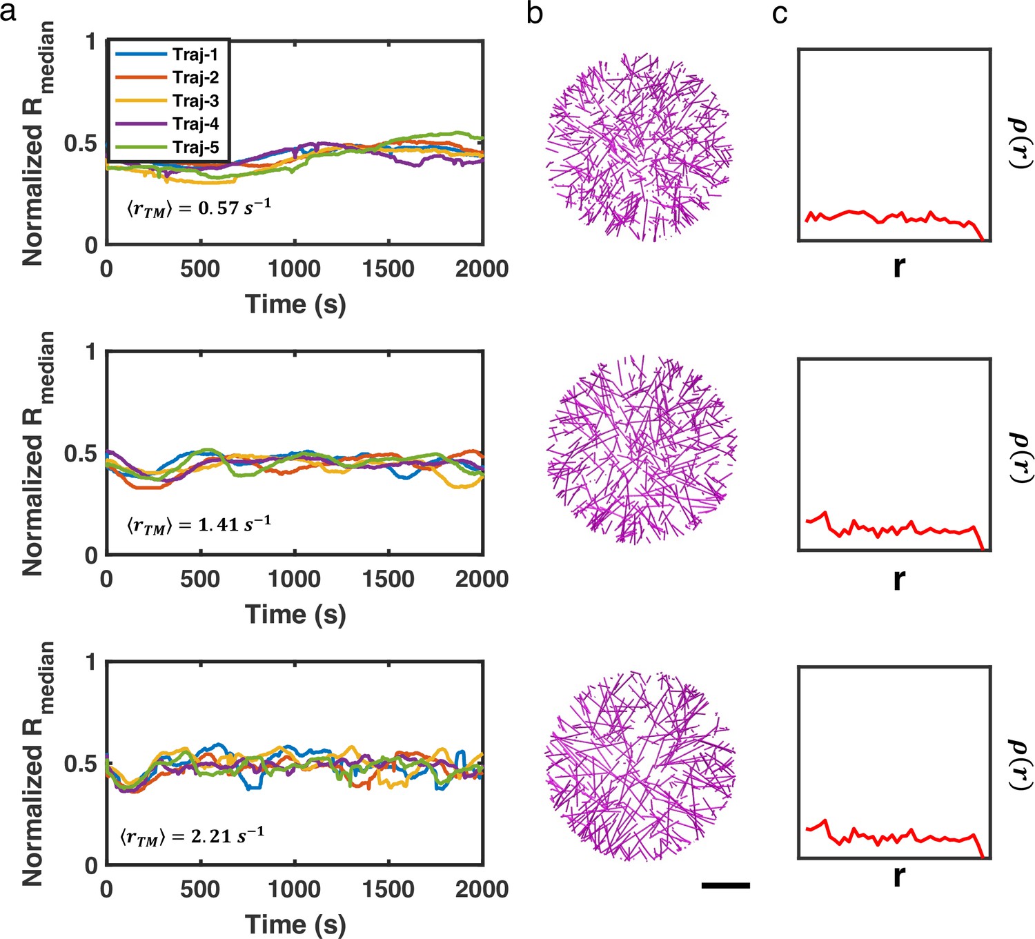
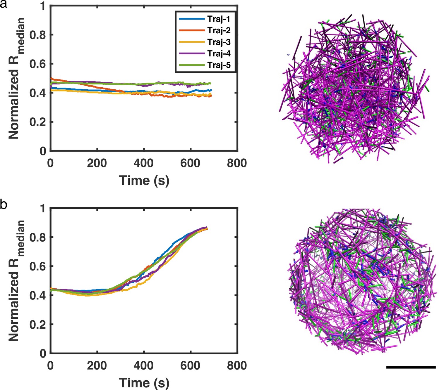
Actin networks remain disordered in the absence of myosin, regardless of treadmilling rate.
(a) 5 trajectories of normalized medians of filament radial density distribution, (b) representative snapshots, and (c) the corresponding filament radial density distributions () at t=2000s are shown. Scale bar = 1 µm.
Figure 2—figure supplement 2
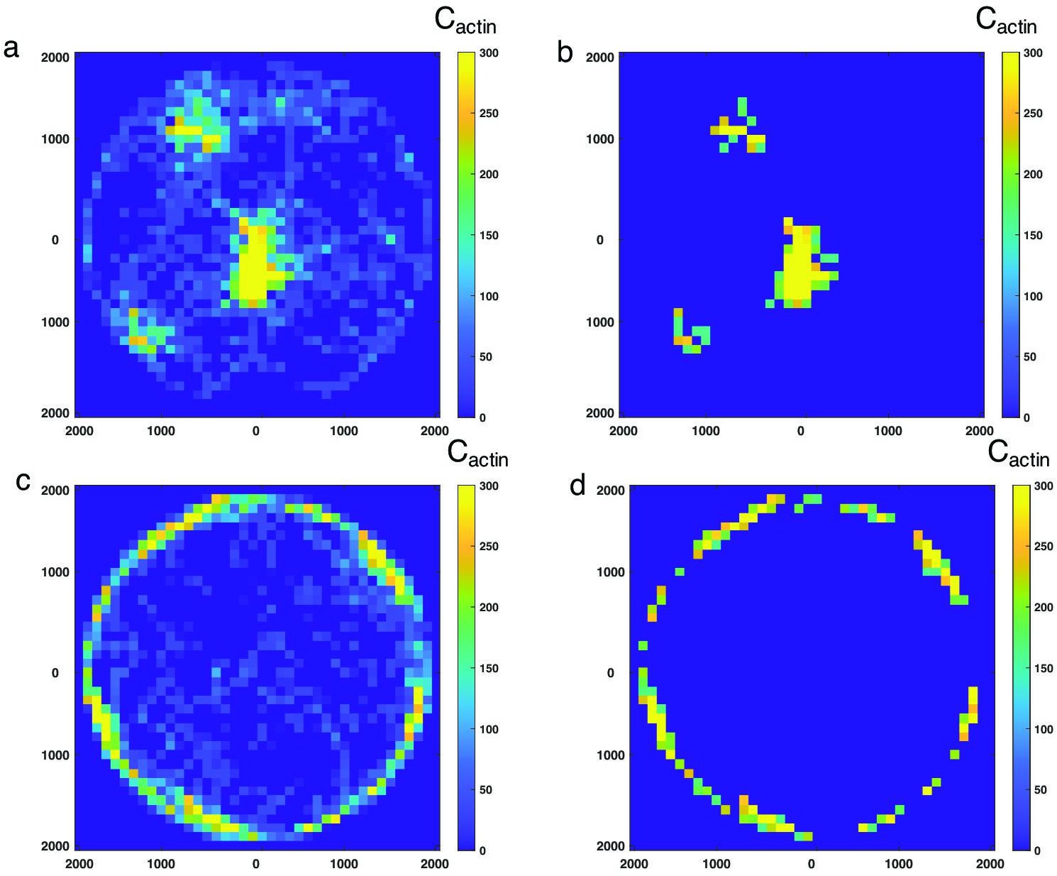
Heatmap showing a pixellated representation of the local F-actin concentration in 100nm x 100nm bins.
(a) A cluster-like network as shown in Figure 1a–c (), and (c) a ring-like network as shown in Figure 1a–c (). (b and d) are the same heatmaps as (a) and (c), respectively, but only contains bins that exceed a concentration threshold of 160µM.
Figure 2—figure supplement 3
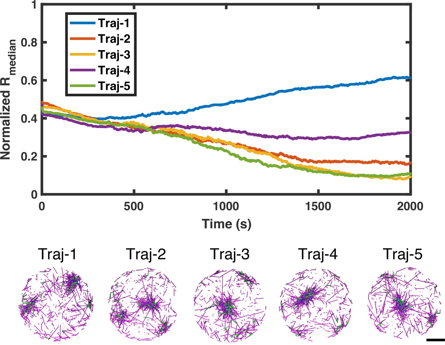
Five trajectories of medians of filament radial density distribution and simulation snapshots with .
The upper plot shows five trajectories of medians of filament radial density distribution with . The lower part shows snapshots of each trajectory at the end of simulation. Actin is in magenta, NMII in green, and crosslinkers in blue. Scale bar =1 µm.
Figure 2—figure supplement 4
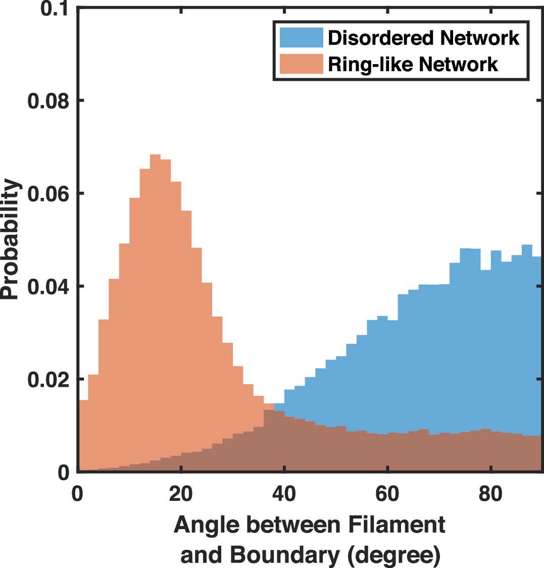
The distribution of filament orientations for disordered networks and ring-like networks near the network periphery .
The distribution of filament orientations for disordered networks () and ring-like networks () near the network periphery (r>1600 nm) are shown. More filaments are oriented perpendicular to the boundary in disordered networks. The filament orientation is represented by the angle between the treadmilling direction (the non-bendable barbed end cylinder) and the tangent vector to the boundary. Only filaments longer than 200nm are counted. The angle ranges from to , with indicating treadmilling parallel to the boundary and indicating treadmilling perpendicular to the boundary. Five runs per condition.
Figure 2—figure supplement 5
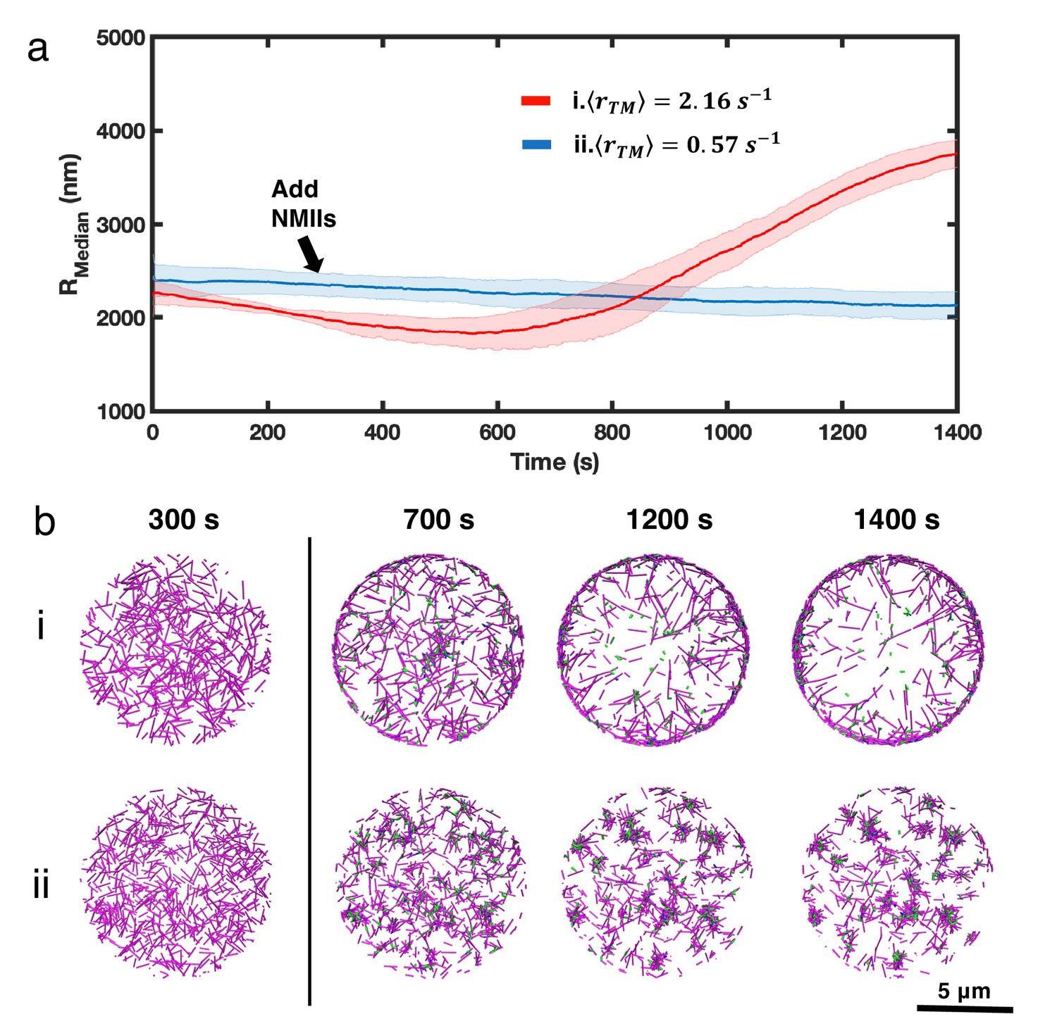
Comparison of network evolution under different treadmilling conditions in a larger, 10 µm geometry.
(a) Medians of filament radial density distribution () at different treadmilling rates () are shown. Networks are simulated in a thin oblate geometry, which has a diameter of 10µm and a height of 200nm. The network contains 20µM G-actin and 30nM filament nucleator. 0.03µM of NMII and 2µM alpha-actinin are added at t=301s. Shahded error bars indicate the standard deviation across five runs. (b) Snapshots of the evolution of representative networks under high treadmilling (i) and low-treadmilling (ii) conditions. Actin is shown in magenta, NMII in green, and crossklinkers in blue. Scale bar = 5 µm.
Figure 2—figure supplement 6
Evolution of three dimensional actin networks under different treadmilling conditions.
(a–b) Median of filament radial density distribution () at different treadmilling rates () and the most representative snapshots in spherical networks are shown. The diameter of the spherical network is 4 µm. The network contains 20µM G-actin and 20nM filament nucleators. 0.03 µM of NMII and 2µM alpha-actinin are added at t=50 s. Scale bar = 1µm.
Figure 2—figure supplement 7
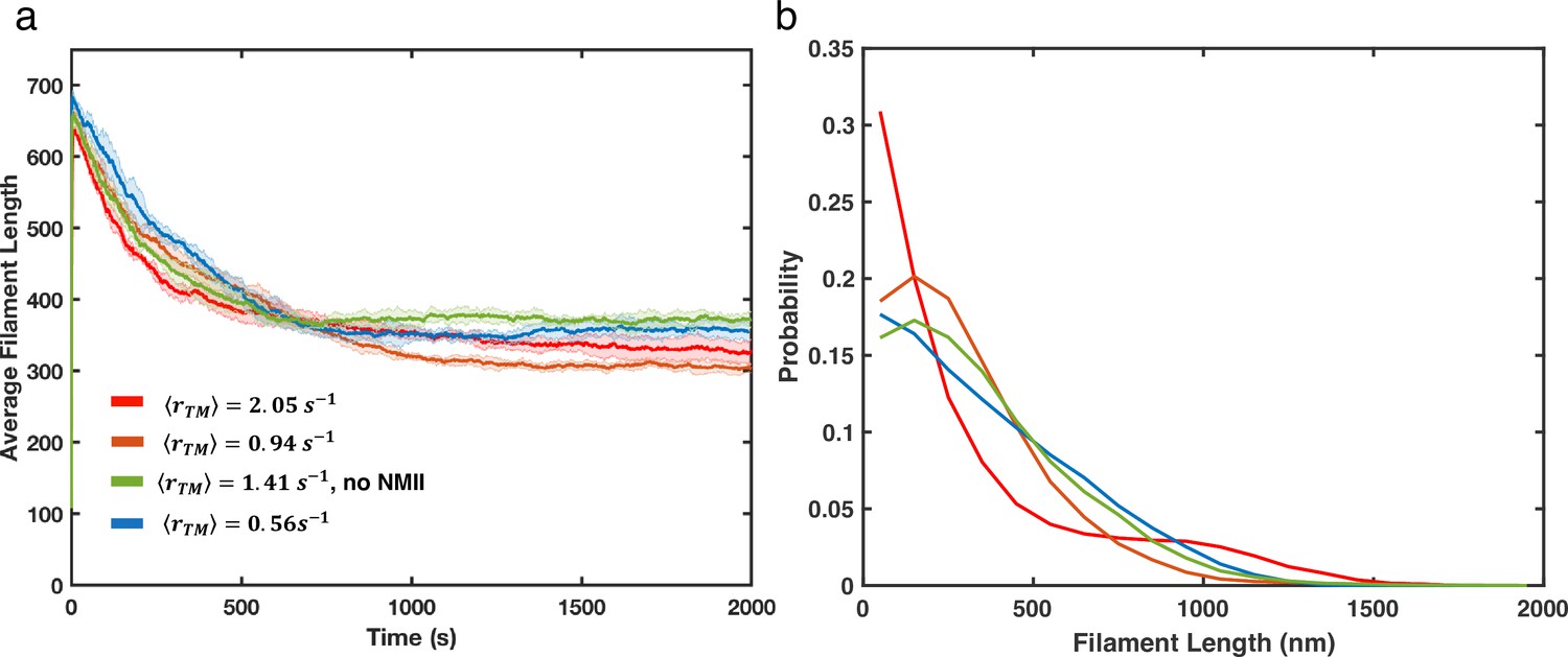
Actin filament length distributions under different treadmilling conditions.
(a) Average filament lengths as a function of time are shown for different treadmilling rates with colors as indicated in the legend. Shaded color represents the standard deviation of mean (5 runs per condition). (b) Filament length distribution (last 500s) at different treadmilling rates with the same color legend as panel a.
Figure 2—video 1
The simulated actin network either contains only actin filaments (top left), as shown in Figure 2—figure supplement 1, or contains actin filaments, myosin, and crosslinkers (top right, bottom left and right) with average tradmilling rate and , respectively, as shown in Figure 2a–b.
Actin filaments are magenta cylinders, and NMIIs are green cylinders. Scale bar = 1 µm.
Figure 2—video 2
Myosin motors bend actin filaments in fast treadmilling networks.
During actin ring formation, actin filaments (red cylinders) change their orientation from perpendicular to the boundary to parallel to the boundary. Some filaments are highlighted with black to emphasize this deformation. NMIIs are blue cylinders.
Figure 2—video 3
The evolution of a fast-treadmilling network in a spherical boundary as shown in Figure 2e.
Actin filaments are magenta cylinders, and NMIIs are green cylinders. Scale bar = 1 µm.
Figure 3 with 1 supplement

Treadmilling rate and NMII concentration regulate network structure transitions.
(a) Normalized medians of radial filament density distribution () as a function of time at different (0.56 to 2.05 ) are shown. The shaded colors represent the standard deviation of means for 5 runs. (b) The box plot shows the average in the last 500 s of simulation at each treadmilling rate. Solid line connects the mean at each . (c) The box plot shows the speed of network remodeling, measured as the slope of the linear part of after 300 s. The solid line connects the mean remodeling rates at each . (a–c) . (d) Steady state at different (0.56 to 2.05 ) and (0.02–0.2 µM). (e) Representative snapshots of steady state actin network structures at different and . Representative snapshots of trajectories in (a) are shown in the dashed box. (d-e) . Actin is depcited as magenta cylinders and NMII as green cylinders. Scale bar = 2 µm.
Figure 3—figure supplement 1
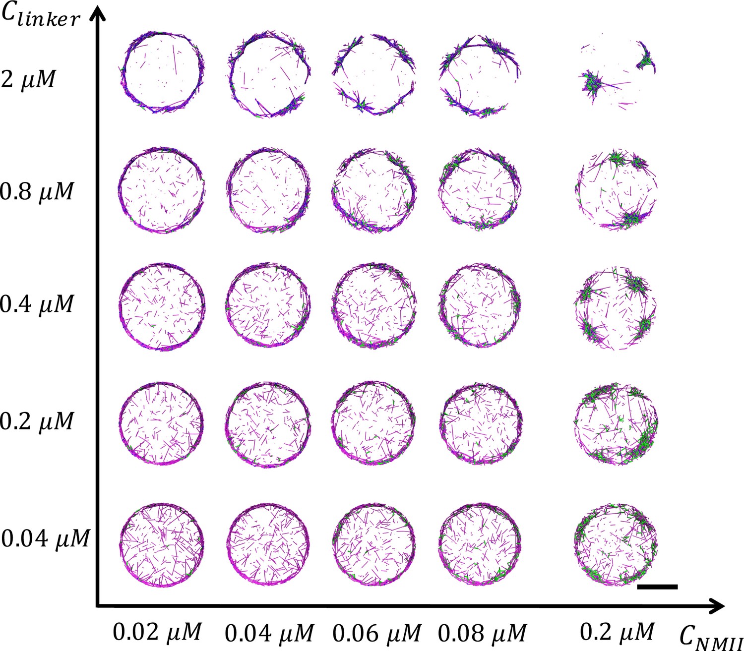
Representative snapshots of steady state actin network structures at different and for all conditions.
Actin is in magenta, NMII is in green, and alpha-actinin is in blue. Scale bar = 2 µm.
Figure 4 with 2 supplements

Inhibition of actin dynamics induces collapse of actin rings in live T cells and in silico.
(a–c) Timelapse montages of Jurkat T cells expressing F-tractin-EGFP spreading on anti-CD3 coated glass substrates. Cells were treated with (a) vehicle control (0.1% DMSO), (b) 250 nM LatA, or (c) 500 nM LatA between 300 and 360 s after contact with activating surface. The first post-treatment image is labeled as 0 s. Timelapse images illustrate the centripetal collapse of the actin ring upon treatment with LatA. Timescales of this collapse depend on the concentration of LatA as can be seen from the timestamps on the images. Scale bar is 10 µm. (d) Quantification of the spatial organization of the actin network using the normalized median of radial filament density distribution. Shaded error bars represent the standard deviations across trajectories (7–11 cells per condition). (e) Box plots showing the rate of centripetal collapse, measured as the slope of the distribution after inhibition. (f–h) Timelapse montages of simulations of (f) control, (g) weak inhibition, and (h) strong inhibition. Treadmilling rates in these conditions are , , and , respectively. Indicated is the averaged treadmilling from 1500 s to the end of simulations. Scale bar indicates 1 µm. (i) Medians of radial filament density distribution at different conditions. (j) Rate of centripetal collapse, measured as the slope of the distribution after inhibition. (i, j) The shaded color and error bars represent the standard deviation across trajectories, n=5 runs per condition.
Figure 4—video 1
Timelapse movie of F-tractin-EGFP labeled F-actin in Jurkat T cells activated by anti-CD3 coated stimulatory coverslips with 0.1% DMSO (vehicle control), and with 250 nM, 500 nM, and 1 µM LatA, respectively.
Vehicle (DMSO) or inhibitor are added as indicated in the movie . Scale bar is 10 µm. The first frame after LatA or DMSO addition is timestamped as T=0.
Figure 4—video 2
Simulation of actin assembly disruption in ring-like actin networks to mimic LatA inhibition in experiments.
The network is allowed to evolved for 800 seconds with as shown in Figure 2—video 1 before the disruption of actin filament polymerization and depolymerization. Actin filaments are magenta cylinders, and NMII are green cylinders. Scale bar = 1 µm.
Figure 5 with 4 supplements
Enhancement or inhibition of NMII regulates actin structure in live T cells and in silico.
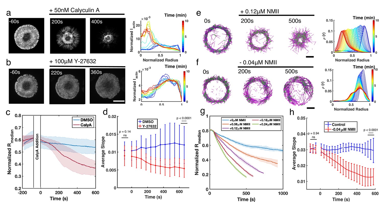
(a–b) Time lapse montages of Jurkat T cells expressing F-tractin-EFGP spreading on anti-CD3-coated glass substrates (left) and the normalized radial F-actin intensity (right). After achieving maximal spreading, cells were treated with (a) 50 nM CalyA, or (b) 100 µM Y-27632. Scale bar is 10 µm. (c) The normalized median of radial filament density distribution . n=12 cells for vehicle (0.5% DMSO), and n=14 cells for CalyA. Two sample t-test was performed for the first point before drug addition (ns, p=0.83) and 600 s after drug addition (****, p<0.0001). (d) The slope of the intensity profiles over the transition region from the center to the peripheral plateau as a function of time. n=25 cells for vehicle (0.1% DMSO), and 24 for Y-27832. Two sample t-test was performed for the first point (before drug addition) and the last point (660 s after drug addition). (e–f) Timelapse montages of simulations (left) and the normalized radiaul filament density distribution at different times (right) mimicking actin rings in (e) CalyA treatment by increasing NMII levels, and (f) Y-27632 treatment by reducing NMII levels. An actin ring containing 80 µM actin, 0.18 µM NMII, and 4 µM alpha-actinin was pre-initialized as described in the Simulation Methods, and the NMII perturbation was performed at 0 s. The control condition is shown in Figure 5—figure supplement 2. Scale bar is 1 µm. (g) The evolution of for different levels of NMII addition. Blue curve is control, and other curves are simulations with indicated levels of NMII added to mimic the CalyA experiment. (h) The slope of the intensity profiles over the transition region from the center to the peripheral plateau as a function of time for simulations of Y-27632 addition. Blue curve is control while orange curve represents simulations after reduction of NMII concentration by 0.04 µM. Two sample t-test was performed for the first three points (before inhibition) and the last three points (510 s to 600 s after drug addition). (g–h) n=5 runs per condition. (a–h) In all figures, 0 s represented the first time point recorded after drug addition (for experiments) or NMII addition/depletion (for simulations). (c,d,g,h) Shaded colors and error bars represent the standard deviation across cells or simulation trajectories.
Figure 5—figure supplement 1
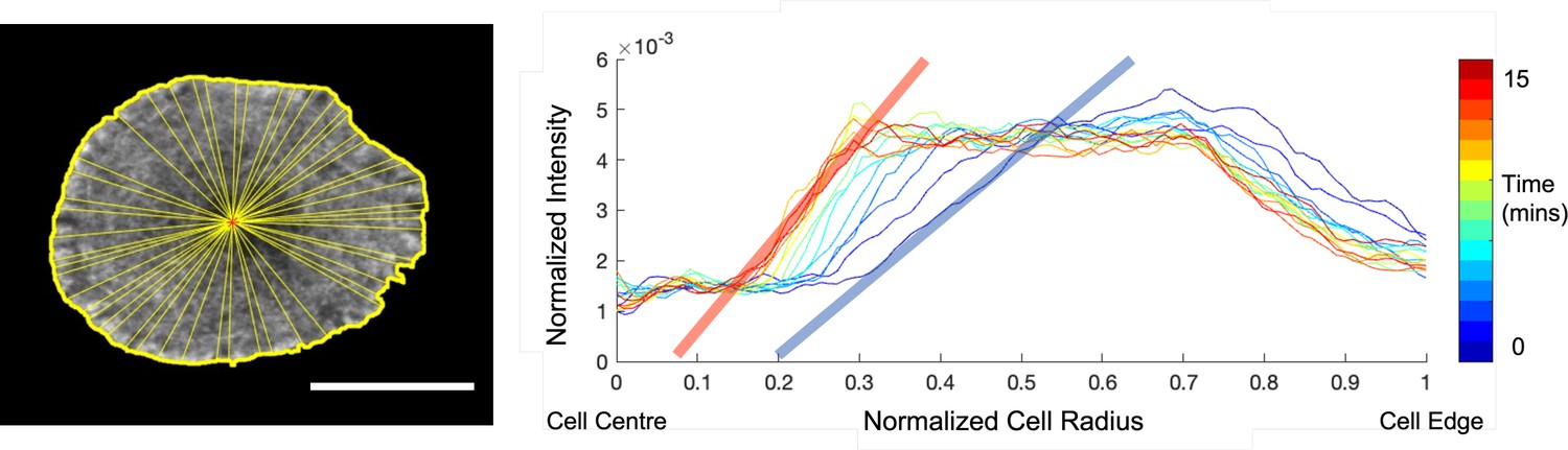
An example for calculating the slope of center to plateau F-actin distribution.
(Left) Example image of a Jurkat T cell expressing F-Tractin-EGFP with the cell mask (yellow outline) and centroid (red asterisk) overlaid. 50 equally spaced lines joining the centroid to the mask edge are randomly drawn (yellow). The average intensity profile over these lines is generated to produce. a single intensity line profile from the cell centroid to the cell edge for a cell at a given time point. (Right) Normalized F-actin intensityprofiles for the cell shown on the left at selected timepoints (indicated as per the color bar) 30 seconds apart for the duration of imaging. Linear fits for the steeply increasing region of the normalized F-actin intensity profiles (shaded red and blue lines) are used to calculate the slope of center to plateau F-actin distribution at each time point. Scale bar is 10 µm.
Figure 5—figure supplement 2
Actin ring dynamics in live T cells and in silico under control conditions in the absence of inhibitions.
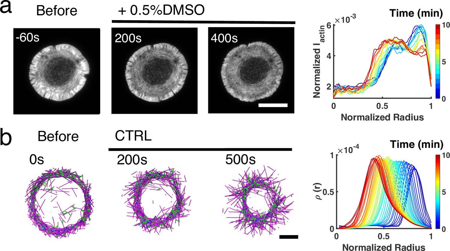
(a–b) Time lapse montages of Jurkat T cells expressing F-tractin-EFGP spreading on anti-CD3 coated glass substrates (left) and the normalized radial F-actin intensity at different times (right). After achieving maximal spreading, cells were treated with 0.5% DMSO. Scale bar is 10 µm. (b) Timelapse montages of simulations (left) and the normalized radial filament density distribution at different times (right) mimicking actin rings in vehicle control. Scale bar is 1 µm.
Figure 5—video 1
Timelapse movie of F-tractin-EGFP labeled F-actin in Jurkat T cells activated by anti-CD3 coated stimulatory coverslips and treated with 50 nM CalyA and 100 µM Y-27632, respectively.
Scale bar is 10 µm. The first frame after drug or DMSO addition is timestamped as T=0.
Figure 5—video 2
Simulations of hyper-activating and inhibiting NMII in ring-like actin networks to mimic CalyA and Y-27632 treatment, as shown in Figure 5.
Networks were pre-assembled into actin rings during the initial 100 s before hyper-activating and inhibiting NMII. Actin filaments are magenta cylinders, and NMIIs are green cylinders. Scale bar = 1 µm.
Figure 6 with 1 supplement
Energetic origins of actin rings.
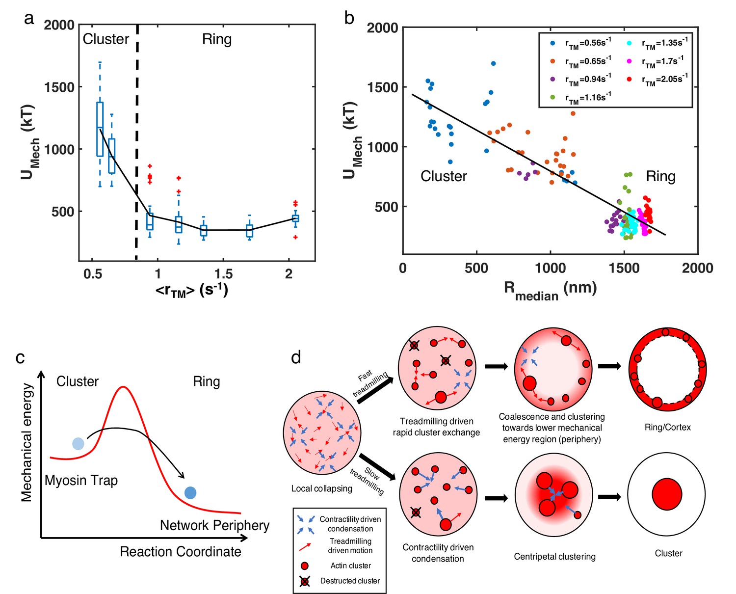
(a) The box plot shows the steady state at each treadmilling rate. is the sum of the bending energy of actin filaments and the stretching energy of filaments, motors, and linkers. The solid line connects the mean at each . (b) Mechanical energy () and the corresponding at different as indicated in the legend. Each data point represents the average and per 100 s of the last 500 s of simulation. (a–b) , with varying as shown in Figure 3a–c. n=5 runs per condition. (c) A graphical description showing the proposed energy landscape for generating actin cortices. (d) Schematic showing the formation of actin ring/cortex versus clusters. At low treadmilling rates, networks are dominated by myosin-driven contraction, leading to centripetal collapse into clusters (lower). Faster filament treadmilling allows networks to overcome the myosin-driven centripetal motion, where filaments tend to move to the network periphery due to lower energy (upper).
Figure 6—figure supplement 1
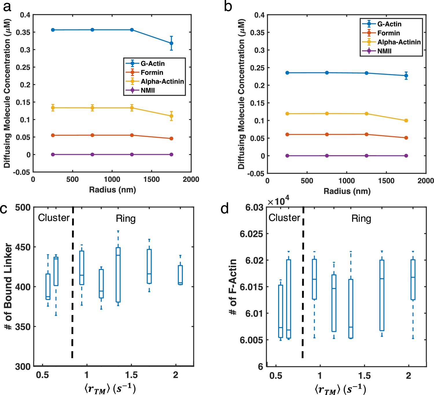
Soluble molecules show no spatial dependence in clustered or ring-like networks.
(a–b) Diffusing molecule concentrations along the radius of (a) cluster networks () and (b) ring-like networks (, b) are shown. (c–d) Box plots of the number of (c) bound linkers and (d) F-actin in the system are shown. Almost all motors are bound upon addition, thus we do not provide a plot for the number of bound motors.
Tables
Table 1
Mechanical parameters.
| Names | Parameters | References |
|---|---|---|
| Cylinder stretching | Popov et al., 2016 | |
| Cylinder bending | Ott et al., 1993 | |
| Filament volume exclusion | Popov et al., 2016 | |
| Linker stretching | DiDonna and Levine, 2007 | |
| NMII stretching | per head | Vilfan and Duke, 2003 |
| Boundary repulsion | This work |
Table 2
Parameters for diffusion and reactions.
| Names | Parameters | References |
|---|---|---|
| Diffusion | Hu and Papoian, 2010 | |
| Actin | 32 and this work | |
| Destruction | This work | |
| Nucleation | Ni and Papoian, 2019 | |
| Formin dissociation | Fritzsche et al., 2016 | |
| Alpha-actinin | Wachsstock et al., 1993 | |
| NMII head binding | Kovács et al., 2003 | |
| Popov et al., 2016 |
Table 3
Mechanochemical dynamic rate parameters.
| Names | Parameters | References |
|---|---|---|
| Characteristic polymerization force | Footer et al., 2007 | |
| Characteristic linker unbinding force | Ferrer et al., 2008 | |
| NMII duty ratio | Kovács et al., 2003 | |
| NMII stall force | per head | Erdmann et al., 2013 |
| Tunable parameters | Popov et al., 2016 | |
Additional files
Download links
A two-part list of links to download the article, or parts of the article, in various formats.
Downloads (link to download the article as PDF)
Open citations (links to open the citations from this article in various online reference manager services)
Cite this article (links to download the citations from this article in formats compatible with various reference manager tools)
A tug of war between filament treadmilling and myosin induced contractility generates actin rings
eLife 11:e82658.
https://doi.org/10.7554/eLife.82658


