Network instability dynamics drive a transient bursting period in the developing hippocampus in vivo
- Department of Neurology, Jena University Hospital, Germany
- Section Translational Neuroimmunology, Jena University Hospital, Germany
- Department of Psychology, Technical University Dresden, Germany
- Department of Neurophysiology, Institute of Physiology, University of Würzburg, Germany
Figures
Figure 1
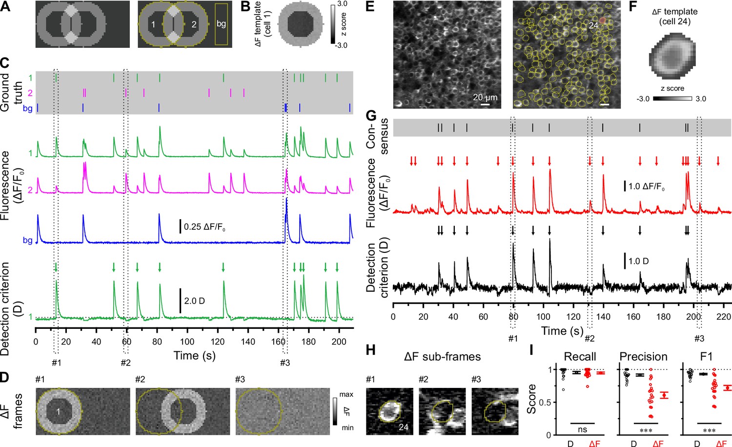
Calcium transient detection harnessing spatial similarity (CATHARSiS) enables reliable Ca2+ transient (CaT) detection in densely labeled tissue.
(A) Resting image of two partially overlapping simulated cells (left) and regions of interest (ROIs) used for analysis (right). bg – background. (B) ΔF template of cell 1. (C) Top, simulated trains of action potentials. Middle, relative changes from baseline fluorescence (ΔF/F0) of ROIs shown in A. Bottom, detection criterion (D) for cell 1 and corresponding CaT onsets retrieved by CATHARSiS (arrows). (D) Sample ΔF images of three individual frames at time points indicated in C. Spikes in cells 1 or 2 translated into ring-shaped increases in ΔF, whereas those induced by bg spikes were applied to the entire field of view. (E) Resting GCaMP6s fluorescence image (left) and ROIs used for analysis (right). (F) ΔF template of the cell indicated in E. (G) Top, consensus visual annotation by two human experts for the same cell. Middle, ΔF/F0 and detected event onsets (red arrows). Bottom, detection criterion (D) and corresponding CaT onsets retrieved by CATHARSiS (black arrows). (H) Sample ΔF images of three individual frames at time points indicated in G. Note that frames #2 and #3 led to false positive results if event detection was performed on mean ΔF, but not if performed on D. (I) Quantification of recall, precision, and F1 score for event detection based on D (i.e. CATHARSiS) and mean ΔF, respectively. Each open circle represents a single cell (n = 20 cells). Data are presented as mean ± SEM. ns – not significant. *** p<0.001. See also Supplementary file 1a and Figure 1—source data 1.
-
Figure 1—source data 1
Numerical data presented in Figure 1.
- https://cdn.elifesciences.org/articles/82756/elife-82756-fig1-data1-v1.xlsx
Figure 2
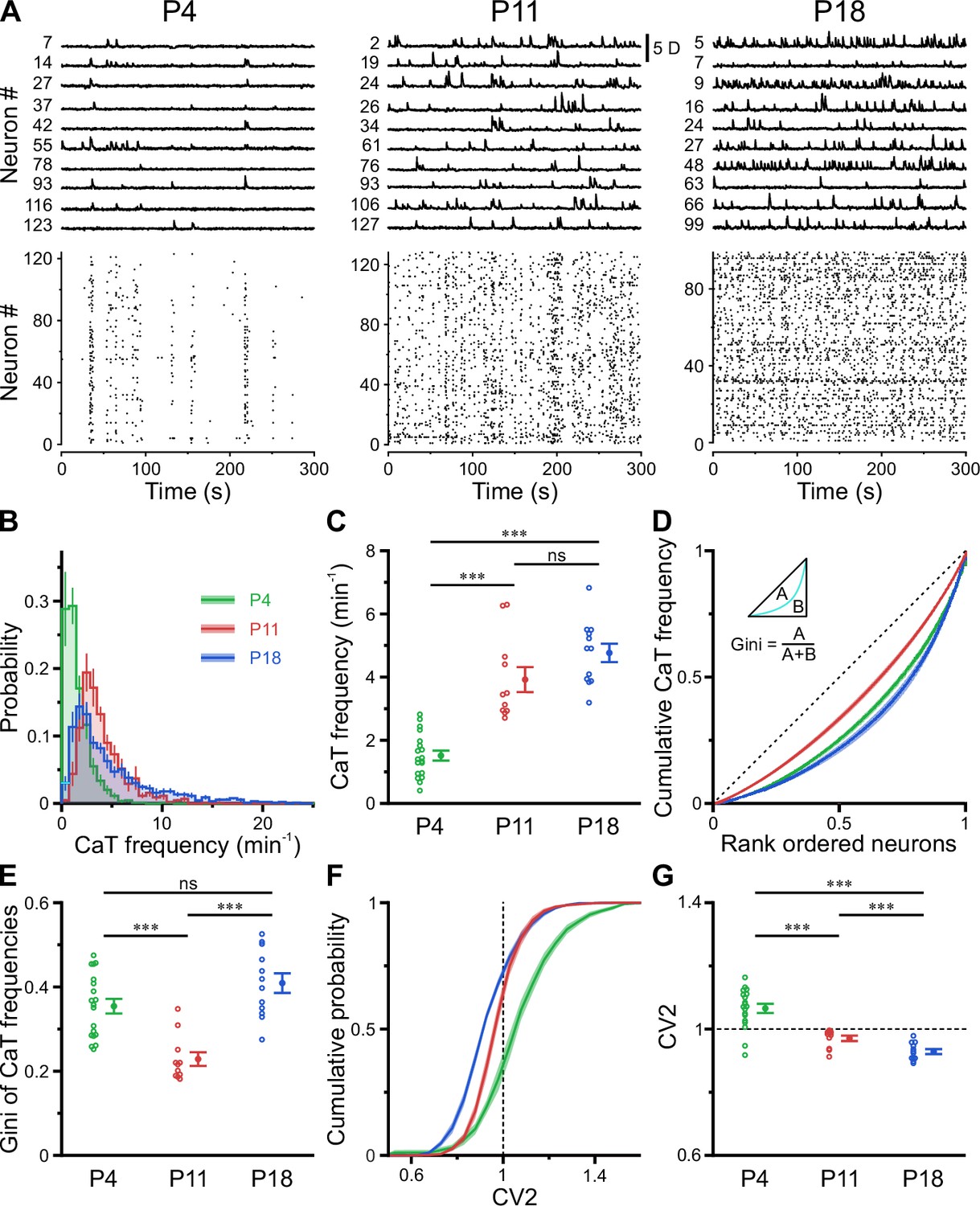
A transient period of firing equalization during CA1 development in vivo.
(A) Sample D(t) traces (top) and raster plots showing reconstructed Ca2+ transient (CaT) onsets (bottom). Note the developmental transition from discontinuous to continuous network activity. (B) Empirical probability distribution of CaT frequencies. (C) Mean CaT frequencies per field of view (FOV). (D) Lorenz curves of CaT frequencies. Line of equality (dotted) represents the case that all neurons have equal CaT frequencies. Inset depicts Gini coefficient calculation. (E) Mean Gini coefficients per FOV. (F) Cumulative probability of mean coefficient of variation (CV2) of inter-CaT intervals. Note that, at P11, CV2 distribution is narrower and centered around 1. (G) Mean CV2 per FOV. For a Poisson process, CV2 = 1 (dotted line). Each open circle represents a single FOV. Data are presented as mean ± SEM. ns – not significant. P4: P3–4, n = 19 FOVs from six mice, P11: P10–12, n = 11 FOVs from six mice, P18: P17–19, n = 12 FOVs from six mice, and *** p<0.001. See also Supplementary file 1b and Figure 2—source data 1.
-
Figure 2—source data 1
Numerical data presented in Figure 2.
- https://cdn.elifesciences.org/articles/82756/elife-82756-fig2-data1-v1.xlsx
Figure 3 with 1 supplement

CA1 undergoes a transient enhanced bursting period while progressively transitioning from discontinuous to continuous activity.
(A) Sample traces of the fraction of active cells Φ(t). Gray and orange bars indicate discontinuous and continuous network activity, respectively. Bottom traces show time periods marked on top (dotted rectangle) at higher temporal resolution. Red dotted lines indicate the activity-dependent thresholds for network burst (NB) detection. (B) Empirical probability distribution of active cells per frame. (C) Continuous activity emerges at P11 and dominates over discontinuous activity at P18. (D) Power spectral density of Φ(t). (E) Bandpower of Φ(t) in the 0.1–0.5 Hz range. (F) The fraction of time that the network spends in NBs peaks at P11. (G) The average NB duration is lowest at P18. (H) Quantification of NB size as the mean fraction of active neurons (corrected for NB threshold as indicated in A). (I) Empirical probability distribution of the fraction of NBs that each cell is participating in. Each open circle represents a single field of view (FOV). Data are presented as mean ± SEM. ns – not significant. P4: P3–4, P11: P10–12, P18: P17–19, *** p<0.001, ** p<0.01, and * p<0.05. See also Supplementary file 1c and Figure 3—source data 1.
-
Figure 3—source data 1
Numerical data presented in Figure 3.
- https://cdn.elifesciences.org/articles/82756/elife-82756-fig3-data1-v1.xlsx
Figure 3—figure supplement 1
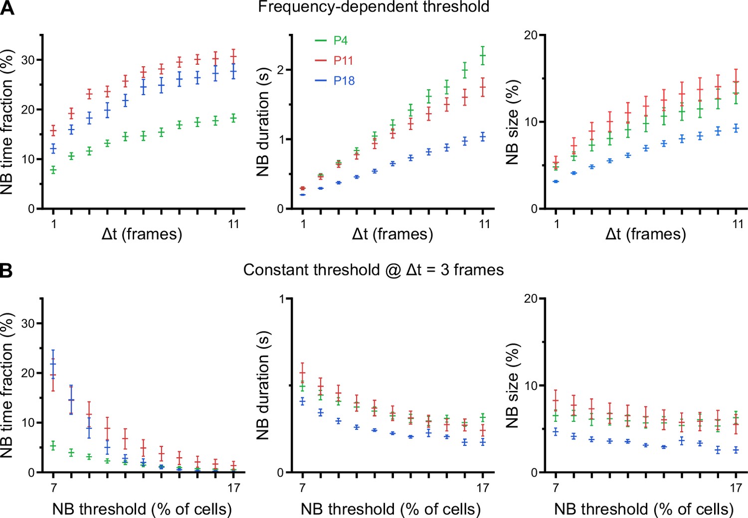
Developmental changes in network burst (NB) characteristics are robust to a wide range of definitions.
(A) Total time spent in NBs (left), mean NB duration (middle), and mean NB size (right) as a function of the parameter Δt. Δt was used for computing a Ca2+ transient (CaT) frequency-dependent threshold, separately for each field of view (FOV; see Methods for details). Sampling rate was 11.63 Hz. (B) Total time spent in NBs (left), mean NB duration (middle), and mean NB size (right) as a function of a constant threshold applied to all FOVs, i.e., independent of CaT frequencies. Note that threshold values below ~10% are less meaningful, as the average fraction of active cells in some FOVs at P18 is ~9%. More generally, for a constant threshold applied to all FOVs, highly active FOVs will be biased toward higher false-positive NB rates, whereas less active FOVs will be biased toward higher false-negative NB rates. Δt was set to 3. See also Figure 3—figure supplement 1—source data 1.
-
Figure 3—figure supplement 1—source data 1
Numerical data presented in Figure 3—figure supplement 1.
- https://cdn.elifesciences.org/articles/82756/elife-82756-fig3-figsupp1-data1-v1.xlsx
Figure 4

Enhanced population coupling (PopC) underlies network burstiness in the second postnatal week in vivo.
(A) The mean PopC index peaked at P11. (B) Mean fraction of cells with significant PopC. (C) Mean PopC index of significantly coupled cells only. (D) Sample spike-time tiling coefficient (STTC) matrices (re-ordered) from three individual fields of view (FOVs) at P4, P11, and P18. (E) Mean fraction of cell pairs having a significant STTC. (F) Cumulative probability of STTCs of significantly correlated cell pairs only. (G) Mean STTCs of significantly correlated cell pairs. (H) Relationship between STTC and Euclidean somatic distance for significantly correlated cell pairs. ρ denotes the Spearman’s rank correlation coefficient for all cell pairs analyzed (n) at a given age. (A–C and E–G) Each open circle represents a single FOV. Data are presented as mean ± SEM. ns – not significant. P4: P3–4, P11: P10–12, P18: P17–19, *** p<0.001, and ** p<0.01. See also Supplementary file 1d and Figure 4—source data 1.
-
Figure 4—source data 1
Numerical data presented in Figure 4.
- https://cdn.elifesciences.org/articles/82756/elife-82756-fig4-data1-v1.xlsx
Figure 5
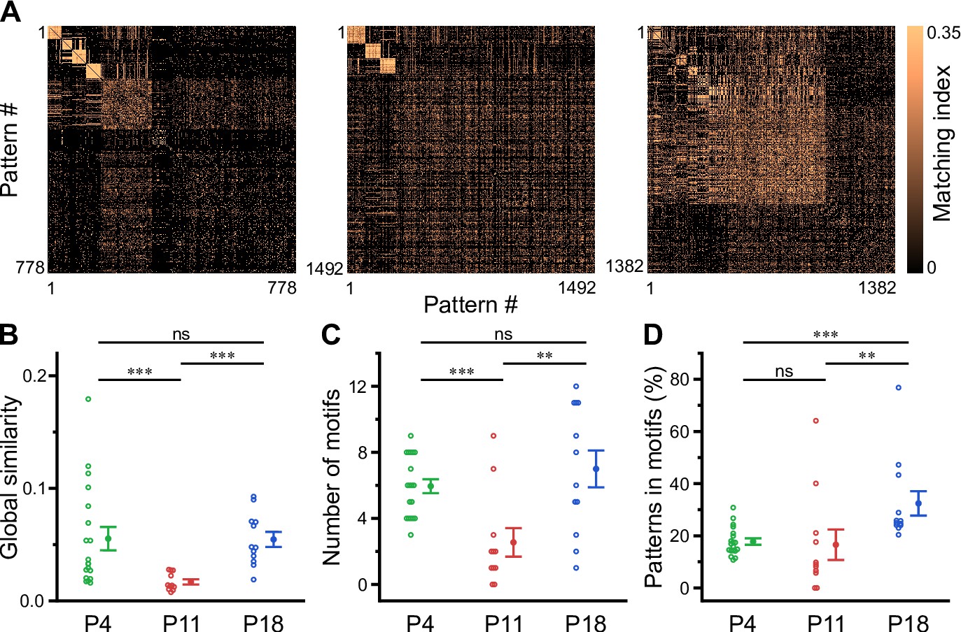
Motifs of CA1 network activity undergo distinct developmental alterations.
(A) Similarity matrices (matching index) of binary activity patterns (re-ordered for illustration of motif detection) from three individual fields of view (FOVs) at P4, P11, and P18. (B) Global similarity of activity patterns is lowest at P11. (C) The absolute number of detected motifs per FOV is lowest at P11. (D) Motif repetition quantified as the fraction of activity patterns belonging to each motif. Each open circle represents a single FOV. Data are presented as mean ± SEM. ns – not significant. P4: P3–4, P11: P10–12, P18: P17–19, *** p<0.001, and ** p<0.01. See also Supplementary file 1e and Figure 5—source data 1.
-
Figure 5—source data 1
Numerical data presented in Figure 5.
- https://cdn.elifesciences.org/articles/82756/elife-82756-fig5-data1-v1.xlsx
Figure 6 with 2 supplements
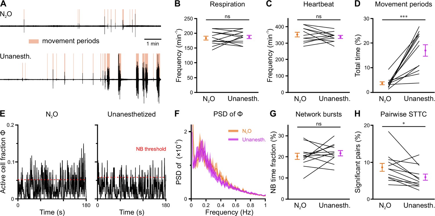
Effects of nitrous oxide (N2O) on body movements, vital parameters, and network activity at P11.
(A) Sample respiration/movement signal from an individual mouse receiving either 75% N2O/25% O2 (top) or pure O2 (Unanesth., bottom). Detected movement periods are highlighted. (B) Respiration rate is unaffected by N2O (n = 12 fields of view [FOVs] from six mice). (C) Heart rate is unaffected by N2O (n = 11 FOVs; in the recording from one FOV, heart rate could not be reliably determined). (D) N2O significantly reduces movement periods. (E) Sample traces of the fraction of active cells Φ(t) (Δt = 3 frames). Red dotted lines indicate the activity-dependent thresholds for network burst (NB) detection. (F) Power spectral density of Φ(t) is similar in the presence or absence of N2O. (G) The fraction of time that the network spends in NBs. (H) Fraction of neuron pairs having a significant spike-time tiling coefficient (STTC). Data are presented as mean ± SEM. ns – not significant. *** p<0.001 and * p<0.05. See also Supplementary file 1f and Figure 6—source data 1.
-
Figure 6—source data 1
Numerical data presented in Figure 6 and Figure 6—figure supplement 2.
- https://cdn.elifesciences.org/articles/82756/elife-82756-fig6-data1-v1.xlsx
Figure 6—figure supplement 1
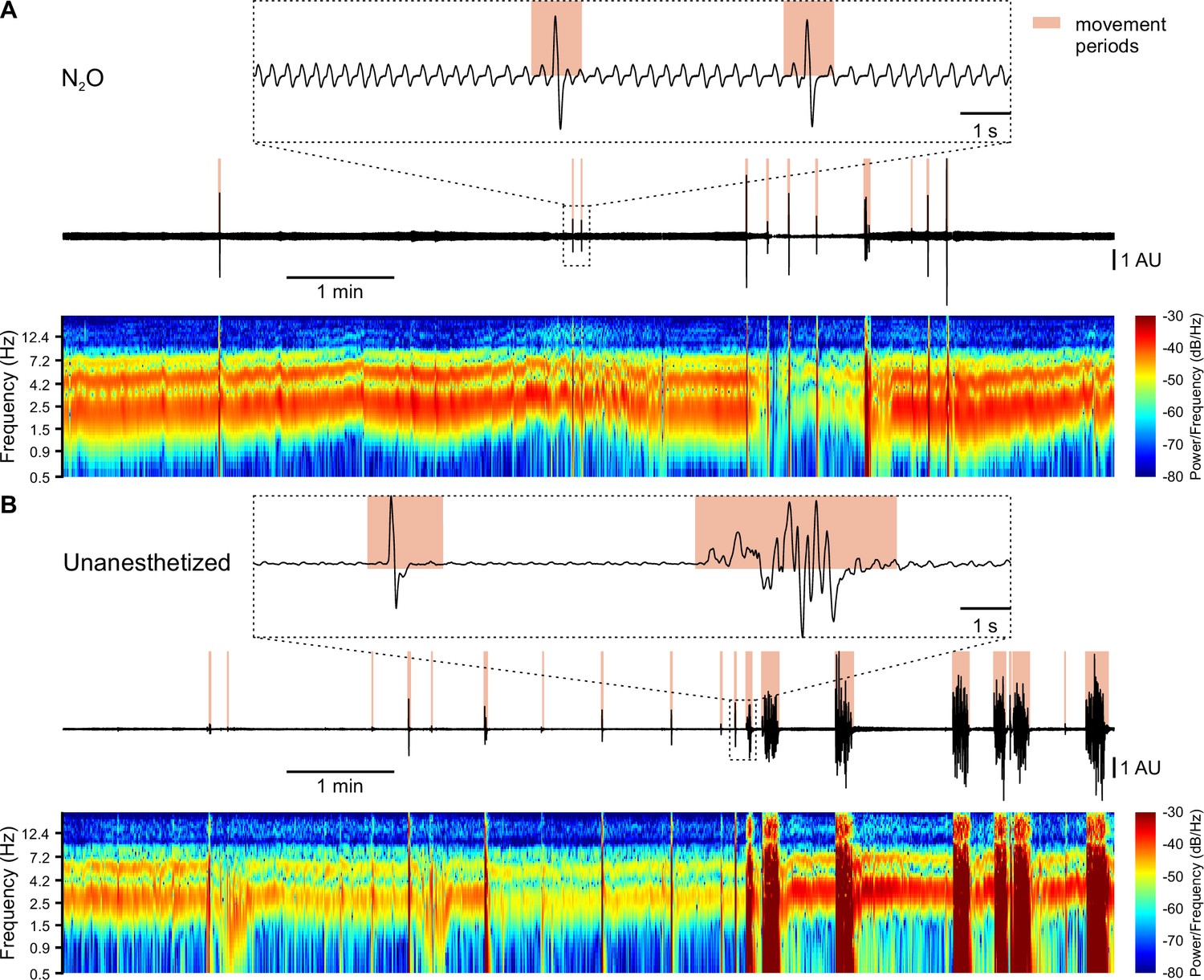
Detection of body movements, breathing, and heart rate.
(A and B) Sample respiration/movement signal (middle) and time-aligned spectrogram (bottom; 0.5–20 Hz, window length: 1 s, overlap: 50%) used to detect movement periods, respiration, and heart rate. Top: marked time periods (dotted rectangle) at higher temporal resolution. Signals were recorded by means of a pressure sensor positioned below the chest of the animal. (A) Recording from an animal receiving 75% N2O/25% O2 (‘N2O’). (B) Recording from the same mouse receiving pure oxygen (‘Unanesthetized’).
Figure 6—figure supplement 2
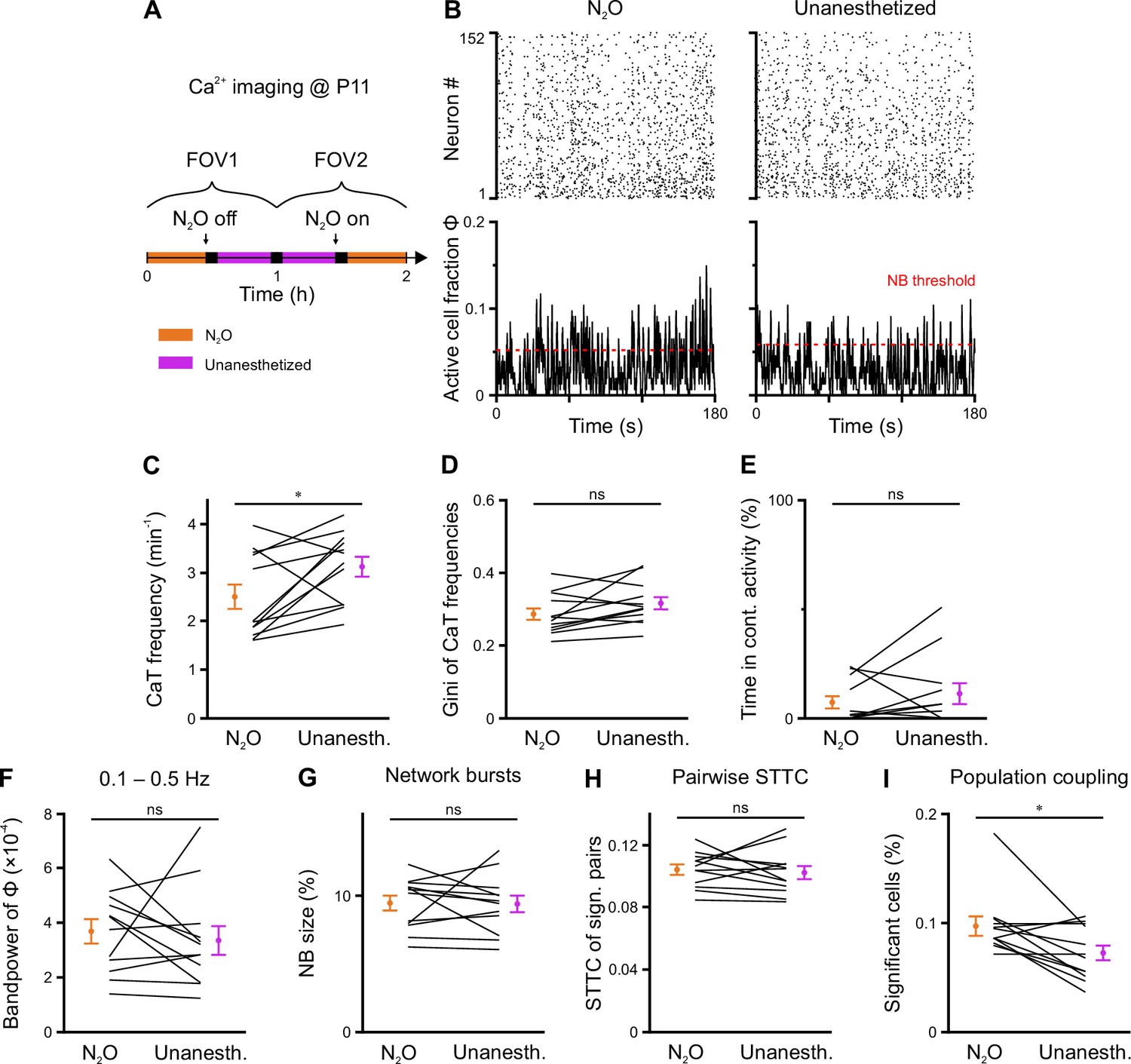
Effects of nitrous oxide on CA1 network dynamics at P11.
(A) Experimental timeline. In each animal, two fields of view (FOVs) were recorded with and without N2O (paired design). (B) Rasterplots (top) and time-aligned fraction of active cells Φ(t) (bottom) from the same FOV in either the presence or the absence of N2O. Red dotted lines indicate the activity-dependent thresholds for network burst (NB) detection. (C) Mean Ca2+ transient (CaT) frequency per FOV. (D) Mean Gini coefficients of CaT frequencies per FOV. (E) Percentage of time spent in continuous activity. (F) Bandpower of Φ(t) in the 0.1–0.5 Hz range. (G) NB size quantified as the mean fraction of active neurons per NB (corrected for burst threshold as indicated in B). (H) Mean spike-time tiling coefficient (STTC) of significantly correlated cell pairs. (I) Mean fraction of cells with significant population coupling (PopC). n = 12 FOVs from six mice, * p<0.05, and ns – not significant. See also Supplementary file 1f and Figure 6—source data 1.
Figure 7

A neural network model with inhibitory GABA identifies intrinsic instability dynamics as key to the emergence of network bursts.
(A) Schematic diagram of the short-term synaptic plasticity (STP)-recurrent neural network (RNN) model. (B) The of the full STP-RNN’s stationary dynamics. Note the presence of two stable fixed points (FPs; green dots) at silent and active states as well as the unstable FP (black dot). (C) Simulated network burst (simNB) generation requires network silencing. The model was stimulated by pulse-like input to both pyramidal cell (PC) and interneuron (IN) populations for a duration of 0.020 s (at t = 3 and 9.2 s: ; at t = 8 s:, ). Zoom-in of the activity around the stimulation times at active (a and b) and silent (c) states is shown in right panels. Input time series are shown on top of the plots. (D) The presence of an amplification domain in the initial phase of network firing dynamics enables the emergence of simNBs. The of the STP-RNN with synaptic efficacies frozen at active (a, top) and silent (b, bottom) states, right before input arrival. (E–G) Transition from active to silent state requires specific input ratios. Input delivered at t = 8 s. (E) A failed transition: , (F) A successful transition: , . (G) A color-coded matrix of successful (dark green) and failed (light green) transitions to the silent state in response to different combinations of and amplitudes. (H–J) Both the transition from the silent to the active state and the simNB generation require specific input ratios. Input delivered at t = 9.2 s. Same as E–G, but for the backward transition to the active state. +simNB and –simNB indicate the emergence and absence of bursts.
Figure 8 with 1 supplement
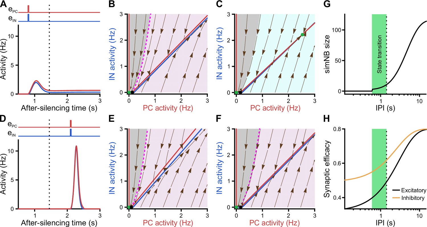
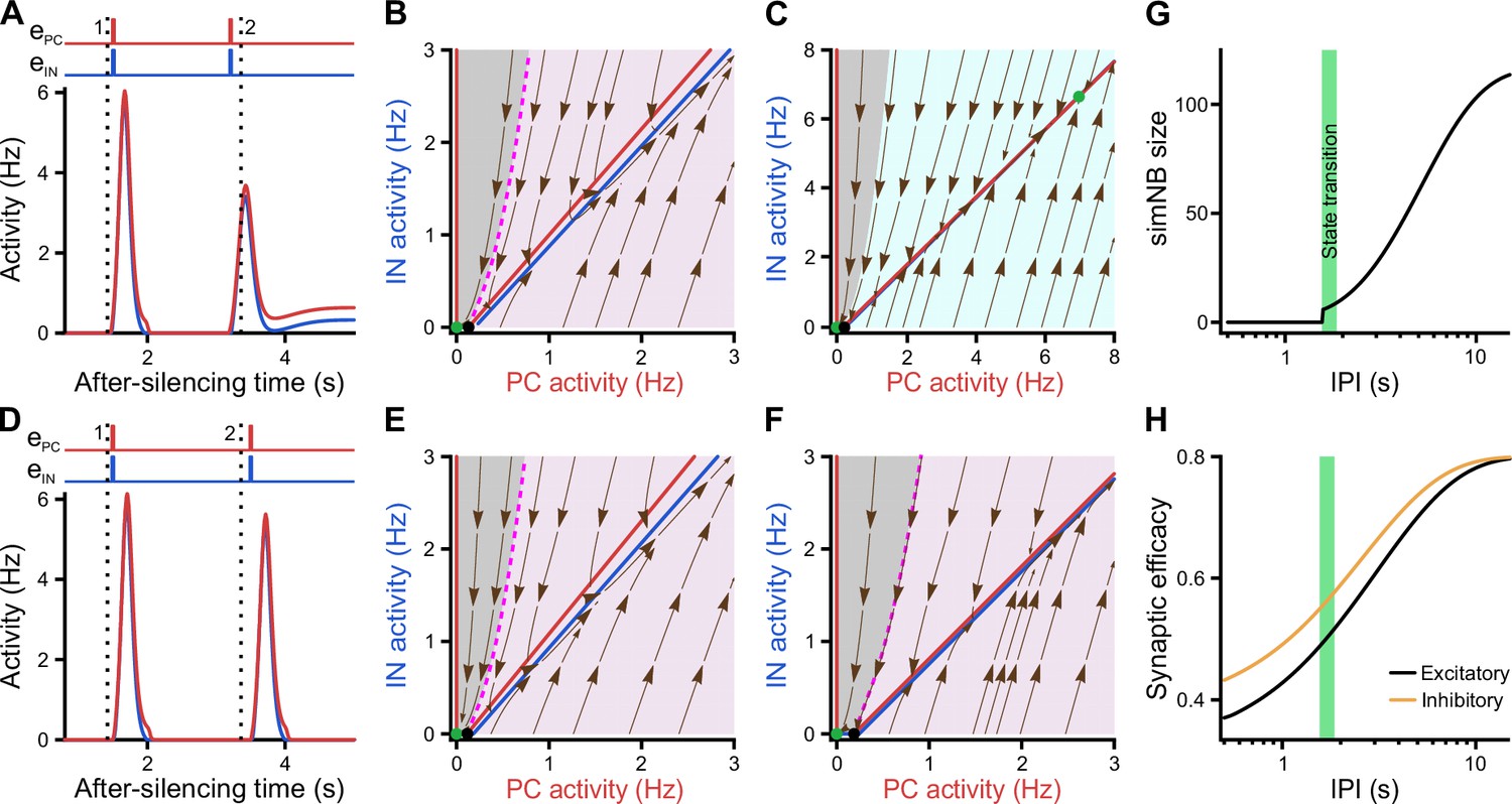
Internal deadline of state transitions.
(A–C) Input delivered to the network before the deadline can move it to active state. (A) A successful transition. The input delivered at t = 0.8 s; , . (B) The of the short-term synaptic plasticity (STP)-recurrent neural network (RNN) with synaptic efficacies frozen at the silent state right before the input arrival. (C) Same as B, but frozen at the peak of the network burst (i.e. simulated network burst [simNB]) shown in A. Note the presence of the transient stable fixed point (FP; non-origin green dot), which triggers the transitioning to the active state. (D–F) Once the deadline is missed, the network cannot be moved to the active state by the subsequent input. Same as A–C, but the input delivered at t = 2.1 s. Note the absence of a non-origin transient stable FP in F, in contrast to C. (G) The simNB size and network transition to the active state depend on the inter-pulse intervals (IPIs: the arrival time of the next input relative to the silencing time of the network). simNB size is computed as the maximum of after the secondary input. Note the presence of a short window for transitioning to the active state. , . (H) Same as G, but for the non-scaled efficacies of GABAergic (; orange; see Methods) and glutamatergic (; black) synapses, right before the arrival of the secondary input. (A, D, G, and H) The dotted line at t = 1.45 s depicts the internal deadline.
Figure 8—figure supplement 1
Re-emergence of an internal deadline after a transition failure.
(A–H) Same format as in Figure 8. Following the failure of the network in transitioning to the active state due to missing the deadline (dotted black line #1, at t = 1.45 s), the subsequent input delivered to the network faces a new deadline (#2, at t = 3.36 s), , . (A–C) Input delivered to the network before the new deadline (#2) can move it to the active state. Inputs delivered at t = 1.55 s and t = 3.2 s, relative to the time that the network was silenced (see Figure 7F). (D–F) Once the new deadline (#2) is missed, the network fails to transition to the active state by the input. Inputs delivered at t = 1.55 s and t = 3.5 s. (G) The size of the simulated network burst (simNB) and the network transition to the active state depend on the inter-pulse interval (IPI). (H) Same as G, but for the non-scaled efficacies of GABAergic and glutamatergic synapses, right before the arrival of the third input. The first input pulse used for silencing the network is not shown.
Figure 9 with 1 supplement
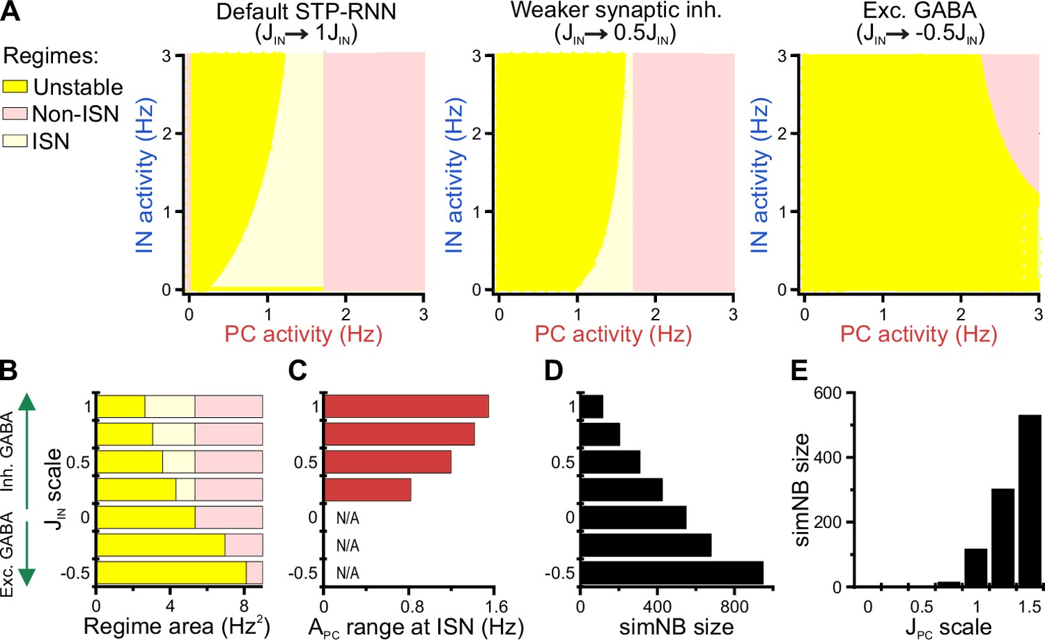
Inhibitory stabilization of a persistent active state in the bi-stable short-term synaptic plasticity (STP)-recurrent neural network (RNN) model.
(A) The inhibition-stabilized network (ISN) regime becomes accessible to the network upon the developmental emergence of synaptic inhibition. The colored regions in each of the network model depict the fixed point (FP)-domains of three possible operating regimes: unstable dynamics, ISN, and Non-ISN. Synaptic inhibition strength was set to 3 (inhibitory; left), 1.5 (inhibitory, middle), and –1.5 (excitatory, right). (B–D) Effect of strength and polarity of GABAergic synapses () on the availability of the ISN regime (B), the maximum range of pyramidal cell (PC) activity in the ISN regime (C), and size of simulated network bursts (simNBs) when triggered at the rest state (D). Results were obtained by scaling in the STP-RNN model with values indicated on the y-axis. The area of each operating regime was computed based on the area of its FP-domain in the (with limits as in A). (E) Dependency of simNB size on the strength of glutamatergic synapses (). Default value of in STP-RNN was 6.5 (corresponding to a scale of 1).
Figure 9—figure supplement 1
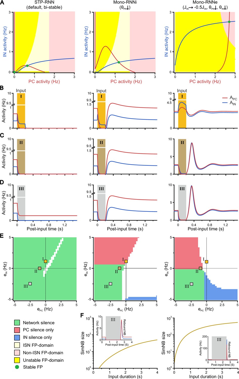
A bi-stable short-term synaptic plasticity (STP)-recurrent neural network (RNN) model with inhibitory GABA robustly explains the experimental observations.
(A) In contrast to the bi-stable STP-RNN, Mono-RNNi and Mono-RNNe networks lack a silent state (i.e. a fixed point [FP] at origin). Same format as Figure 9A, overlaid by the (red), the (blue), and the FPs of each network with dynamic synapses (i.e. 10D system). The unstable FP in the STP-RNN is not shown for clarity. For the exact values of model parameters, see Methods. (B–C) Network responses to example inputs (200 ms; shaded areas). In contrast to the STP-RNN, Mono-RNNi and Mono-RNNe networks can be silenced only during the input. Inputs are: , (B); , (C); (D). (E) In contrast to the STP-RNN, silencing of Mono-RNNi and Mono-RNNe models requires the input (200 ms) to at least one of network populations to be inhibitory. Green indicates complete network silence (), red indicates pyramidal cell (PC) silence only (, ), and blue indicates interneuron (IN) silence only (,). White areas: ,. The activity levels of the neuronal populations were computed as those prior to the input removal. Square symbols (I–III) indicate the input combinations used in panels B–D. (F) In contrast to the STP-RNN, effective (rebound) simulated network burst (simNB) generation in Mono-RNNi (middle) and Mono-RNNe (right) requires a relatively long-lasting input. (Inset) Same as D, but for a longer input of 2 s.
Tables
Key resources table
| Reagent type (species) or resource | Designation | Source or reference | Identifiers | Additional information |
|---|---|---|---|---|
| Strain and strain background (Mus musculus) | B6.129S2-Emx1tm1(cre)Krj/J (Emx1IREScre) | The Jackson Laboratory | RRID: IMSR_JAX:005628 | |
| Strain and strain background (Mus musculus) | B6;129S6-Gt(ROSA)26Sortm96(CAG-GCaMP6s)Hze/J (Rosa26LSL-GCaMP6s) | The Jackson Laboratory | RRID: IMSR_JAX:024106 | |
| Software and algorithm | Wolfram Mathematica 13 | Wolfram | RRID:SCR_014448 | |
| Software and algorithm | Matlab 2021b | Mathworks | RRID:SCR_001622 | |
| Software and algorithm | Fiji | PMID:22743772 | RRID:SCR_002285 | |
| Software and algorithm | Calcium transient detection harnessing spatial similarity (CATHARSiS) | This paper | N/A | https://github.com/kirmselab/CATHARSiS |
Additional files
-
Supplementary file 1
Statistical tests used in this study.
(a) Synopsis of statistical tests related to Figure 1. Numerical data are provided in the Figure 1—source data 1. (b) Synopsis of statistical tests related to Figure 2. Numerical data are provided in the Figure 2—source data 1. (c) Synopsis of statistical tests related to Figure 3. Numerical data are provided in the Figure 3—source data 1. (d) Synopsis of statistical tests related to Figure 4. Numerical data are provided in the Figure 4—source data 1. (e) Synopsis of statistical tests related to Figure 5. Numerical data are provided in the Figure 5—source data 1. (f) Synopsis of statistical tests related to Figure 6 and Figure 6—figure supplement 2. Numerical data are provided in the Figure 6—source data 1.
- https://cdn.elifesciences.org/articles/82756/elife-82756-supp1-v1.docx
-
Transparent reporting form
- https://cdn.elifesciences.org/articles/82756/elife-82756-transrepform1-v1.pdf
Download links
A two-part list of links to download the article, or parts of the article, in various formats.
Downloads (link to download the article as PDF)
Open citations (links to open the citations from this article in various online reference manager services)
Cite this article (links to download the citations from this article in formats compatible with various reference manager tools)
Network instability dynamics drive a transient bursting period in the developing hippocampus in vivo
eLife 11:e82756.
https://doi.org/10.7554/eLife.82756


