Cytoarchitectonic, receptor distribution and functional connectivity analyses of the macaque frontal lobe
- Institute of Neuroscience and Medicine INM-1, Research Centre Jülich, Germany
- Center for Neural Science, New York University, United States
- Bristol Computational Neuroscience Unit, Faculty of Engineering, University of Bristol, United Kingdom
- Center for the Developing Brain, Child Mind Institute, United States
- C. & O. Vogt Institute for Brain Research, Heinrich-Heine-University, Germany
Figures
Figure 1
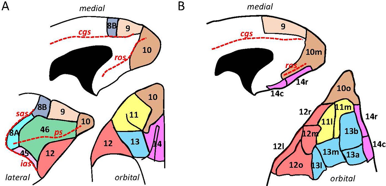
Schematic drawing of the medial, lateral, and orbital surfaces of the macaque prefrontal cortex depicting parcellations according to (A) Walker, 1940, and (B) Carmichael and Price, 1994.
Macroanatomical landmarks are marked with red dashed lines; cgs, cingulate sulcus; ias, inferior arcuate sulcus; ps, principal sulcus; ros, rostral orbital sulcus; sas, superior arcuate sulcus.
Figure 2 with 2 supplements
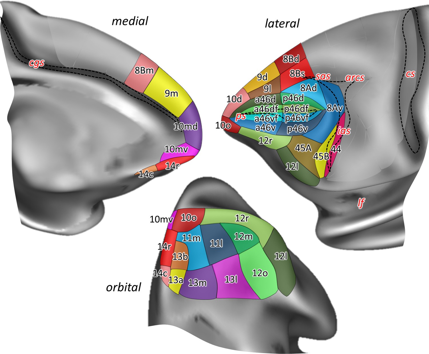
Position and extent of the prefrontal areas on the medial, lateral, and orbital views of the Yerkes19 surface.
The files with the parcellation scheme are available via EBRAINS platform of the Human Brain Project (https://search.kg.ebrains.eu/instances/Project/e39a0407-a98a-480e-9c63-4a2225ddfbe4) and the BALSA neuroimaging site (https://balsa.wustl.edu/study/7xGrm). Macroanatomical landmarks are marked in red letters, while black dashed lines mark fundus of sulci. arcs, spur of the arcuate sulcus; cgs, cingulate sulcus; cs, central sulcus; ias, inferior arcuate sulcus; lf, lateral fissure; ps, principal sulcus; sas, superior arcuate sulcus.
Figure 2—figure supplement 1
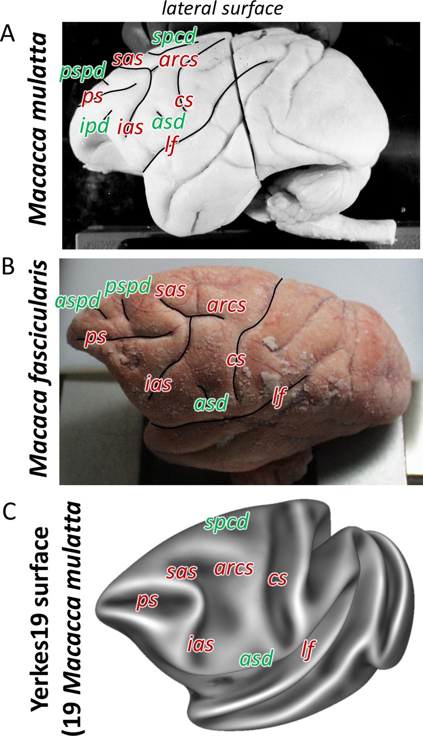
Macroanatomical landmarks (sulci labelled in red letters and dimples in green) shown on the lateral surface of the two related species of macaque monkey used in the present architectonic analyses.
Photographs of two of the postmortem brains used in this study. Brain ID DP1. (A) Macaca mulatta, and brain ID 11530 (B) Macaca fascicularis. Average surface representations of the Yerkes19. (C) Macaca mulatta template brains. arcs, spur of the arcuate sulcus; asd, anterior supracentral dimple; aspd, anterior superior principal dimple; cs, central sulcus; ias, inferior arcuate sulcus; ps, principal sulcus; pspd, posterior superior principal dimple; sas, superior arcuate sulcus; spcd, superior precentral dimple.
Figure 2—figure supplement 2
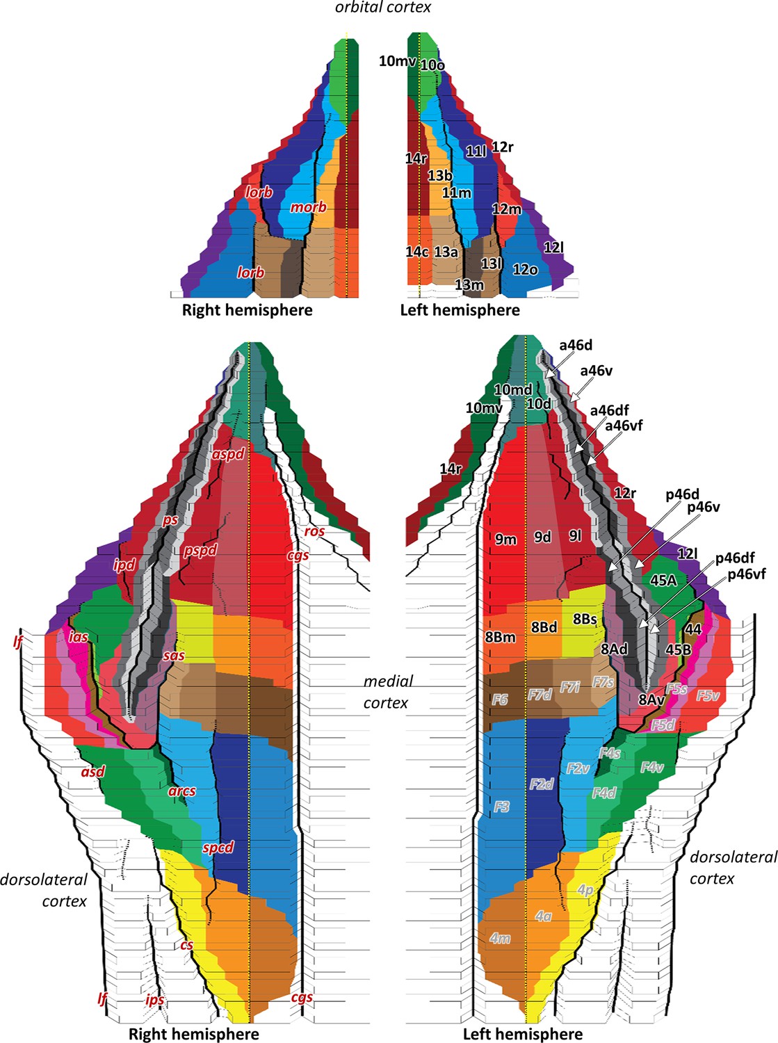
2D flat map, based on the macroanatomical landmarks of every 40th section, displays orbital, medial, and dorsolateral hemispheric views with all defined areas within the macaque frontal lobe.
Areas are labelled on the left hemisphere, that is, prefrontal areas in black and previously mapped (pre)motor areas (Rapan et al., 2021) in grey. Due to limited space on the map, we used white arrows to mark anterior and posterior subdivisions of 46. Dashed yellow line on the hemispheres represents the midline, which separates medial and dorsolateral cortex. Black full lines mark the fundus of sulci. Macroanatomical landmarks are marked on the right hemisphere; arcs, spur of the arcuate sulcus; asd, anterior supracentral dimple; aspd, anterior superior principal dimple; cgs, cingulate sulcus; cs, central sulcus; ias, inferior arcuate sulcus; ipd, inferior principal dimple; lf, lateral fissure; lorb, lateraral orbital sulcus; morb, medial orbital sulcus; ps, principal sulcus; pspd, posterior superior principal dimple; sas, superior arcuate sulcus; spcd, superior precentral dimple.
Figure 3
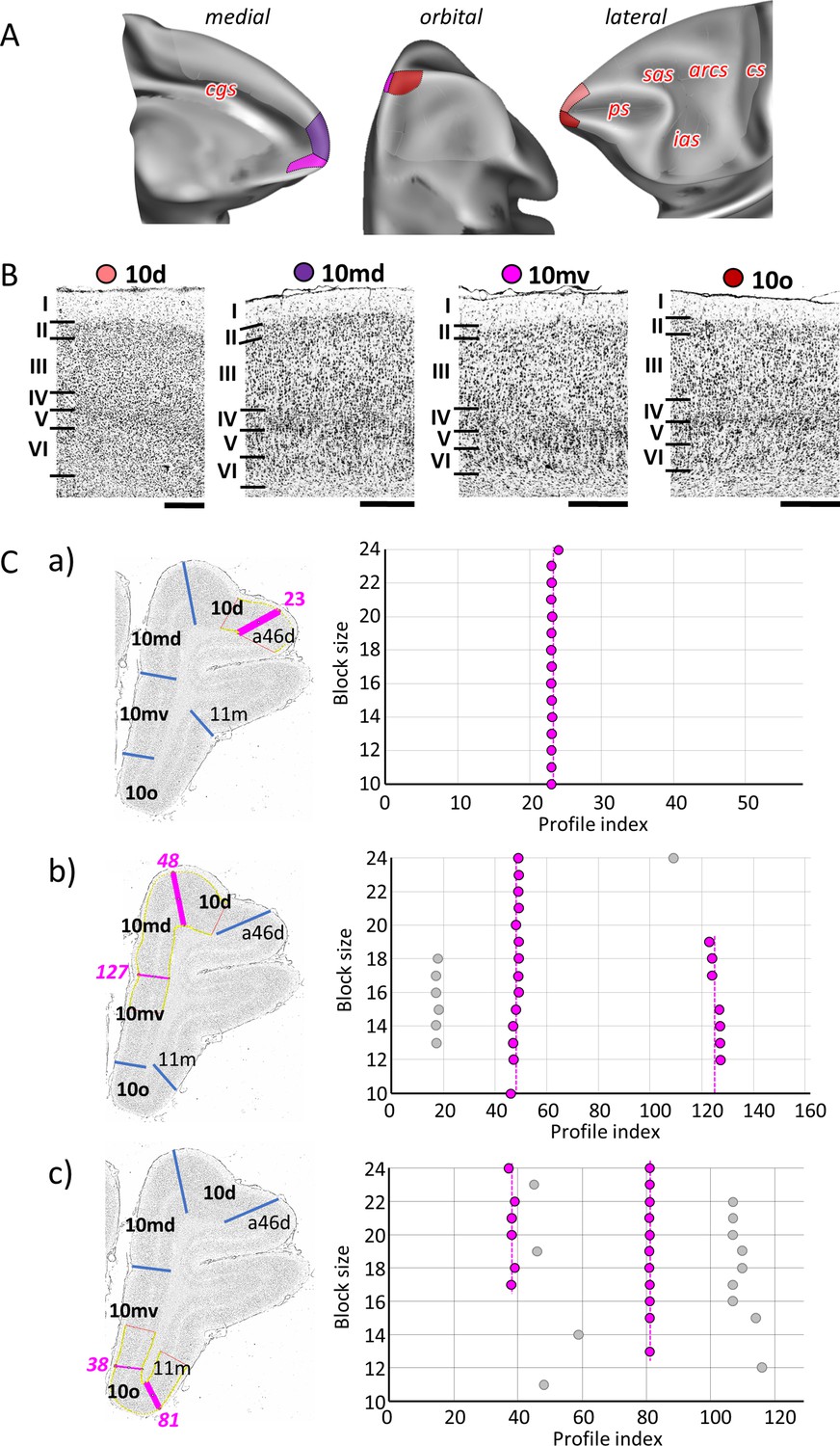
Quantitative analysis of the cytoarchitecture of Walker’s area 10 (Walker, 1940).
(A) Position and extent of subdivisions of Walker’s area 10 within the hemisphere are displayed on orbital, lateral, and medial views of the Yerkes19. Macroanatomical landmarks are marked in red letters. (B) High-resolution photomicrographs show cytoarchitectonic features of areas 10d, 10md, 10mv, and 10o. Each subdivision is labelled by a coloured dot, matching the colour of the depicted area on the 3D model. (C) We confirmed cytoarchitectonic borders by a statistically testable method, where the Mahalanobis distance (MD) was used to quantify differences in the shape of profiles extracted from the region of interest. Profiles were extracted between outer and inner contour lines (yellow lines drawn between layers I/II and VI/white matter, respectively) defined on grey-level index (GLI) images of the histological sections (left column). Pink lines highlight the position of the border for which statistical significance was tested. The dot plots (right column) reveal that the location of the significant border remains constant over a large block size interval (highlighted by the red dots). (a) depicts analysis of the border between areas 10d and a46d (profile index 23); (b) depicts analysis of the border delineating dorsally located subdivisions, 10d and10md (profile index 48), as well as the medial border segregating dorsal and ventral subdivision, 10md and 10mv (profile index 127); and (c) depicts analysis of the borders between ventrally positioned subdivisions of the frontal polar region, 10mv and 10o (profile index 38) and 10o and 11m (profile index 81). Scale bar 1 mm. Roman numerals indicate cytoarchitectonic layers. arcs, spur of the arcuate sulcus; cgs, cingulate sulcus; cs, central sulcus; ias, inferior arcuate sulcus; ps, principal sulcus; sas, superior arcuate sulcus.
Figure 4 with 2 supplements
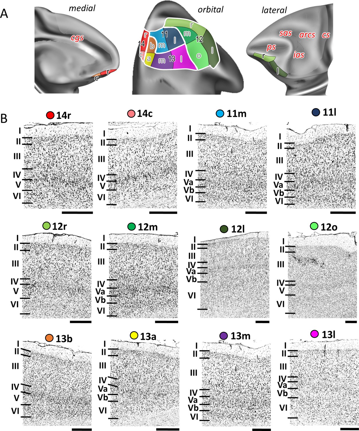
Cytoarchitecture of orbitofrontal areas.
(A) Position and extent of the orbitofrontal areas within the hemisphere are displayed on orbital, lateral, and medial views of the Yerkes19. Macroanatomical landmarks are marked in red letters. (B) High-resolution photomicrographs show cytoarchitectonic features of orbitofrontal 14r, 14c, 11m, 11l, 12r, 12m, 12l, 12o, 13b, 13a, 13m, and 13l. Each subdivision is labelled by a coloured dot, matching the colour of the depict area on the 3D model. Scale bar 1 mm. Roman numerals (and letters) indicate cytoarchitectonic layers. arcs, spur of the arcuate sulcus; cgs, cingulate sulcus; cs, central sulcus; ias, inferior arcuate sulcus; ps, principal sulcus; sas, superior arcuate sulcus.
Figure 4—figure supplement 1
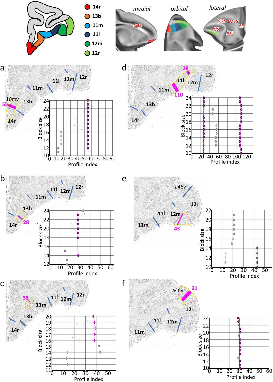
Statistically testable borders (pink lines) confirmed by the quantitative analysis for the rostral orbital and ventrolateral areas 14r, 13b, 11m, 11l, 12m, and 12r.
(a) Border between 14r and 10mv (profile index 55); (b) border between 14a and 13b (profile index 28); (c) border between 13b and 11m (profile index 38); (d) borders between 11m and 11l (profile index 110) and 11l and 12m (profile index 28); (e) border between 12m and 12r (profile index 43); and (f) border between 124 and a46v (profile index 31). For details see Figure 3.
Figure 4—figure supplement 2

Statistically testable borders (pink lines) confirmed by the quantitative analysis for the caudal orbital and ventrolateral areas 14c, 13a, 13m, 13l, and 12o.
(a) Border between 25 and 14c (profile index 26); (b) border between 14c and 13a (profile index 22); (c) border between 13a and 13m (profile index 40); (d) border between 13m and 13l (profile index 59); (e) border between 13l and 12o (profile index 56); and (f) border between 12o and 12l (profile index 76). For details see Figure 3.
Figure 5
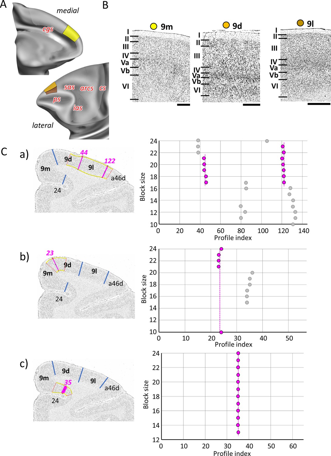
Quantitative analysis of the cytoarchitecture of Walker’s area 9 (Walker, 1940).
(A) Position and extent of the rostral medial and dorsolateral prefrontal areas within the hemisphere are displayed on lateral and medial views of the Yerkes19. Macroanatomical landmarks are marked in red letters. (B) High-resolution photomicrographs show cytoarchitectonic features of areas 9m, 9d, and 9l. Each subdivision is labelled by a coloured dot, matching the colour of the depict area on the 3D model. (C) We confirmed cytoarchitectonic borders by statistically testable method (for details see Figure 3). (a) depicts analysis of the borders between area a46d and 9l (profile index 122), as well as 9l and 9d (profile index 44); (b) depicts analysis of the border between dorsal and medial subdivision, 9d and 9m (profile index 44); and (c) depicts analysis of the border distinguishing medial subdivision 9m from cingulate cortex, area 24 (profile index 35). Scale bar 1 mm. Roman numerals (and letters) indicate cytoarchitectonic layers. arcs, spur of the arcuate sulcus; cgs, cingulate sulcus; cs, central sulcus; ias, inferior arcuate sulcus; ps, principal sulcus; sas, superior arcuate sulcus.
Figure 6
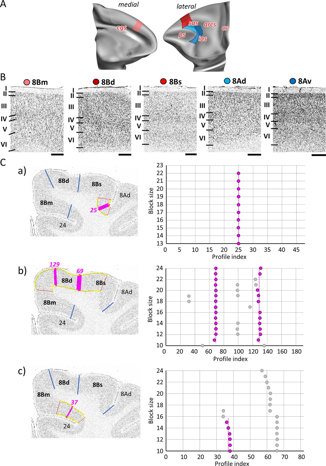
Quantitative analysis of the cytoarchitecture of Walker’s area 8B (Walker, 1940).
(A) Position and the extent of the caudal medial and dorsolateral prefrontal areas within the hemisphere are displayed on lateral and medial views of the Yerkes19. Macroanatomical landmarks are marked in red. (B) High-resolution photomicrographs show cytoarchitectonic features of areas 8B (8Bm, 8Bd, 8Bs) and 8A (8Ad, 8Av). Each subdivision is labelled by a coloured dot, matching the colour of the depict area on the 3D model. (C) We confirmed cytoarchitectonic borders of new 8B subdivisions by statistically testable method (for details see Figure 3). (a) depicts analysis of the border that separates new subdivisions 8Bs from neighbouring area 8Ad (profile index 25); (b) depicts analysis of the borders which delineate area 8Bd from surrounding areas 8Bs and 8Bm (profile index 69), as well as 8Bd and 8Bm (profile index 129); and (c) depicts analysis of the border distinguishing medial subdivision 8Bm from cingulate cortex, area 24 (profile index 37). Statistically testable borders for area 8Ad (adjacent to p46d) shown in Figure 7—figure supplement 2 and for area 8Av borders can be seen in the Figure 8—figure supplement 2. Scale bar 1 mm. Roman numerals (and letters) indicate cytoarchitectonic layers. arcs, spur of the arcuate sulcus; cgs, cingulate sulcus; cs, central sulcus; ias, inferior arcuate sulcus; ps, principal sulcus; sas, superior arcuate sulcus.
Figure 7 with 2 supplements
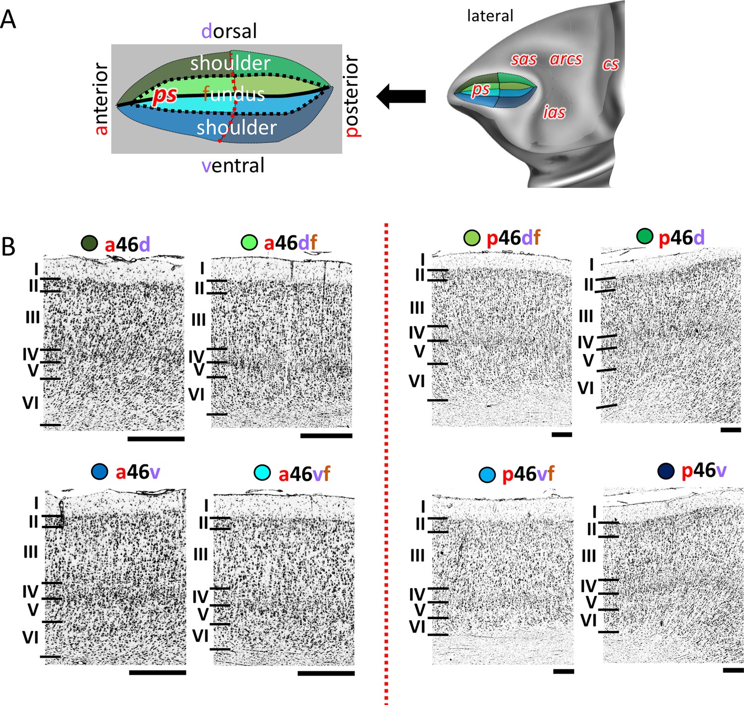
Cytoarchitecture of Walker’s area 46 (Walker, 1940).
(A) Position and the extent of areas located within and around the ps, are displayed on lateral view of the Yerkes19. Additionally, schematic drowning demonstrates how identified subdivisions are labelled with letters highlighted in red. Macroanatomical landmarks are marked in red letters. Black line indicates fundus, black dotted line marks border between shoulder and fundus region, and red dotted line separates anterior and posterior portion of sulcus. (B) High-resolution photomicrographs show cytoarchitectonic features of anterior areas of 46 (a46d, a46df, a46vf, a46v) and posterior ones (p46d, p46df, p46vf, p46v), separated by red dashed line. Each subdivision is labelled by a coloured dot, matching the colour of the depict area on the 3D model. Scale bar 1 mm. Roman numerals indicate cytoarchitectonic layers. arcs, spur of the arcuate sulcus; cs, central sulcus; ias, inferior arcuate sulcus; ps, principal sulcus; sas, superior arcuate sulcus.
Figure 7—figure supplement 1
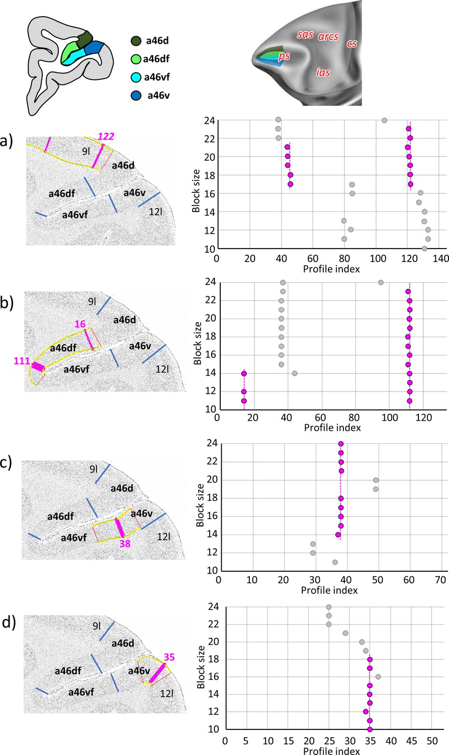
Statistically testable borders (pink lines) confirmed by the quantitative analysis for the rostral region of the ps, occupied by the anterior subdivisions of area 46; a46d, a46df, a46vf, and a46v.
(a) Border between 9l and a46d (profile index 122); (b) borders between a46d and a46df (profile index 16) and a46df and a46vf (profile index 111); (c) border between ap46vf and a46v (profile index 38); and (d) border between a46v and 12l (profile index 35). For details see Figure 3.
Figure 7—figure supplement 2
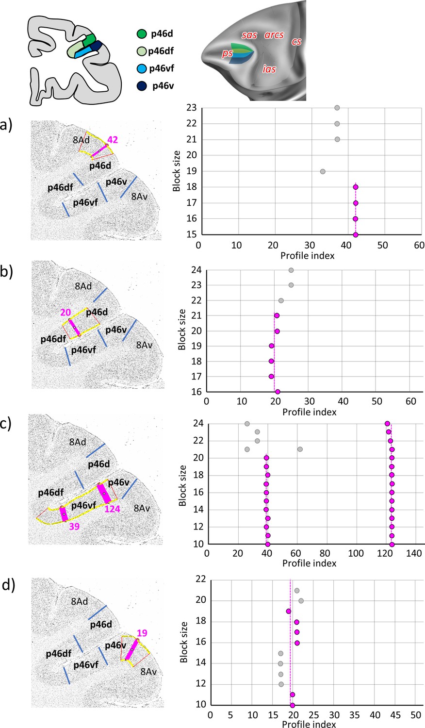
Statistically testable borders (pink lines) confirmed by the quantitative analysis for the caudal region of the ps, occupied by the posterior subdivisions of area 46; p46d, p46df, p46vf, and p46v.
(a) Border between 8Ad and p46d (profile index 42); (b) border between p46d and p46df (profile index 20); (c) borders between p46df and p46vf (profile index 39) and p46vf and p46v (profile index 124); and (d) border between p46v and 8Av (profile index 19). For details see Figure 3.
Figure 8 with 2 supplements
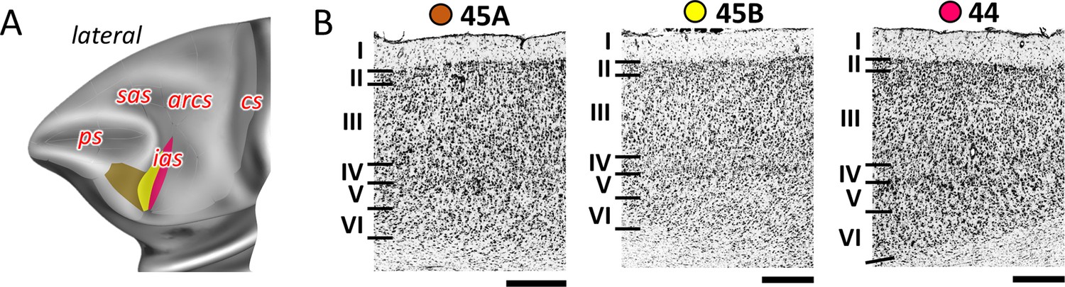
Cytoarchitecture of areas 44 and 45.
(A) Position and the extent of the posterior ventrolateral areas within the hemisphere are displayed on lateral view of the Yerkes19. Macroanatomical landmarks are marked in red letters. (B) High-resolution photomicrographs show cytoarchitectonic features of areas 44 and 45 (45A, 45B). Each subdivision is labelled by a coloured dot, matching the colour of the depict area on the 3D model. Scale bar 1 mm. Roman numerals indicate cytoarchitectonic layers. arcs, spur of the arcuate sulcus; cs, central sulcus; ias, inferior arcuate sulcus; ps, principal sulcus; sas, superior arcuate sulcus.
Figure 8—figure supplement 1
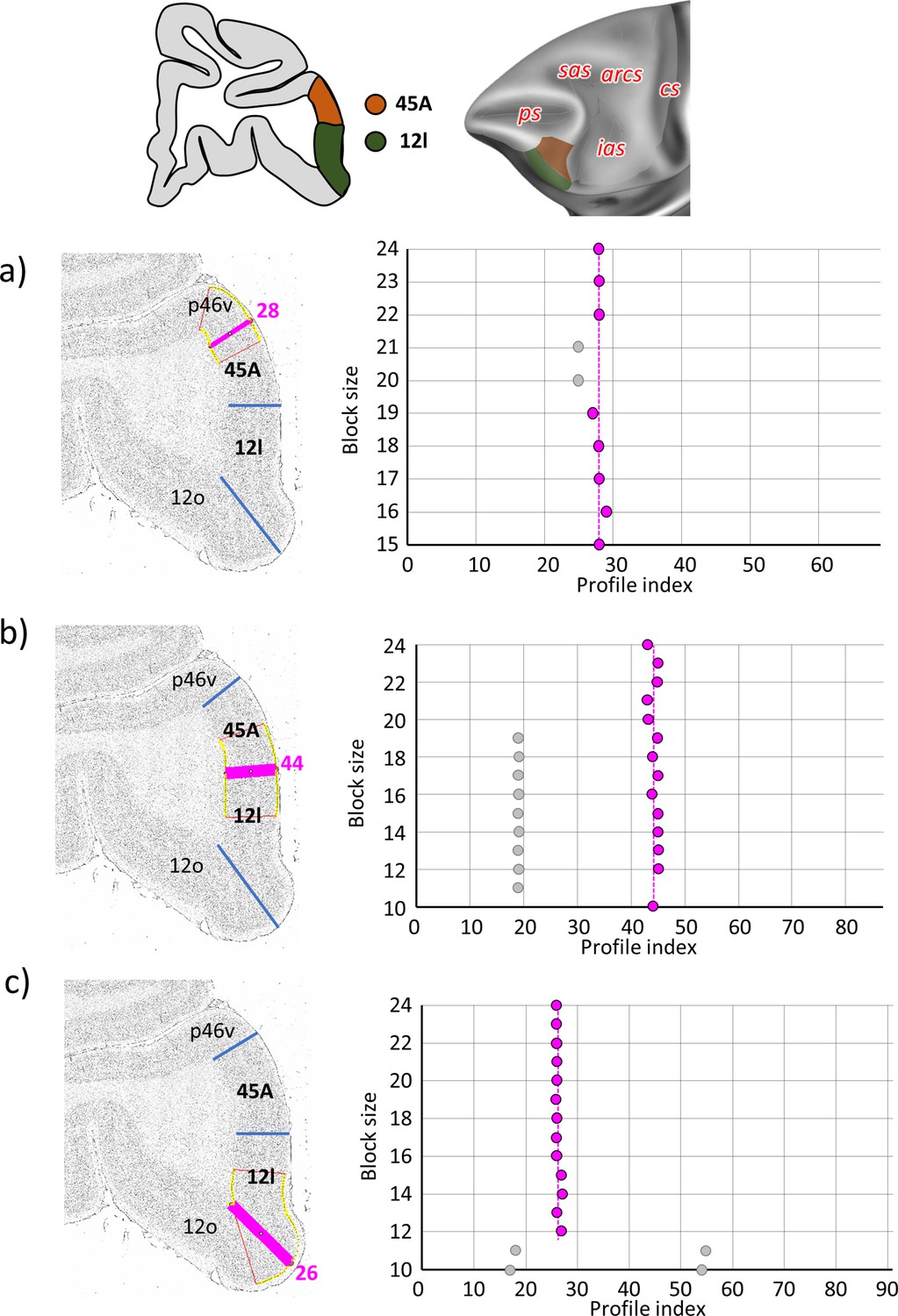
Statistically testable borders (pink lines) confirmed by the quantitative analysis for the caudal ventrolateral area 12l and dorsally adjacent area 45A.
(a) Border between p46v and 45A (profile index 28); (b) border between 45A and 12l (profile index 44); and (c) border between 12l and 12o (profile index 26). For details see Figure 3.
Figure 8—figure supplement 2
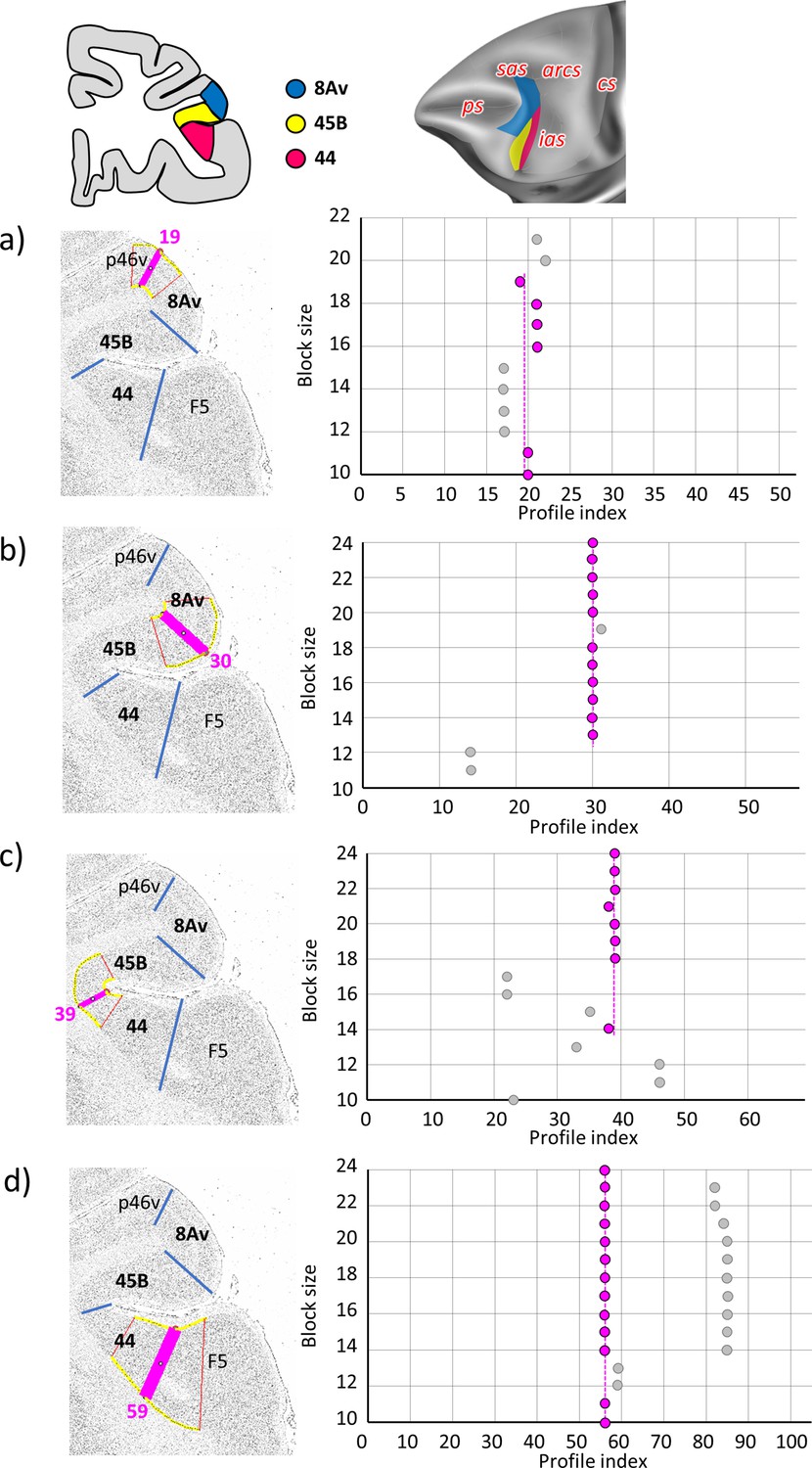
Statistically testable borders (pink lines) confirmed by the quantitative analysis for the caudal ventrolateral cortex; areas 8Av, 45B, and 44.
(a) Border between p46v and 8Av (profile index 19); (b) border between 8Av and 45B (profile index 30); (c) border between 45B and 44 (profile index 39); and (d) border between 44 and F5 (prolfile index 59). For details see Figure 3.
Figure 9 with 3 supplements
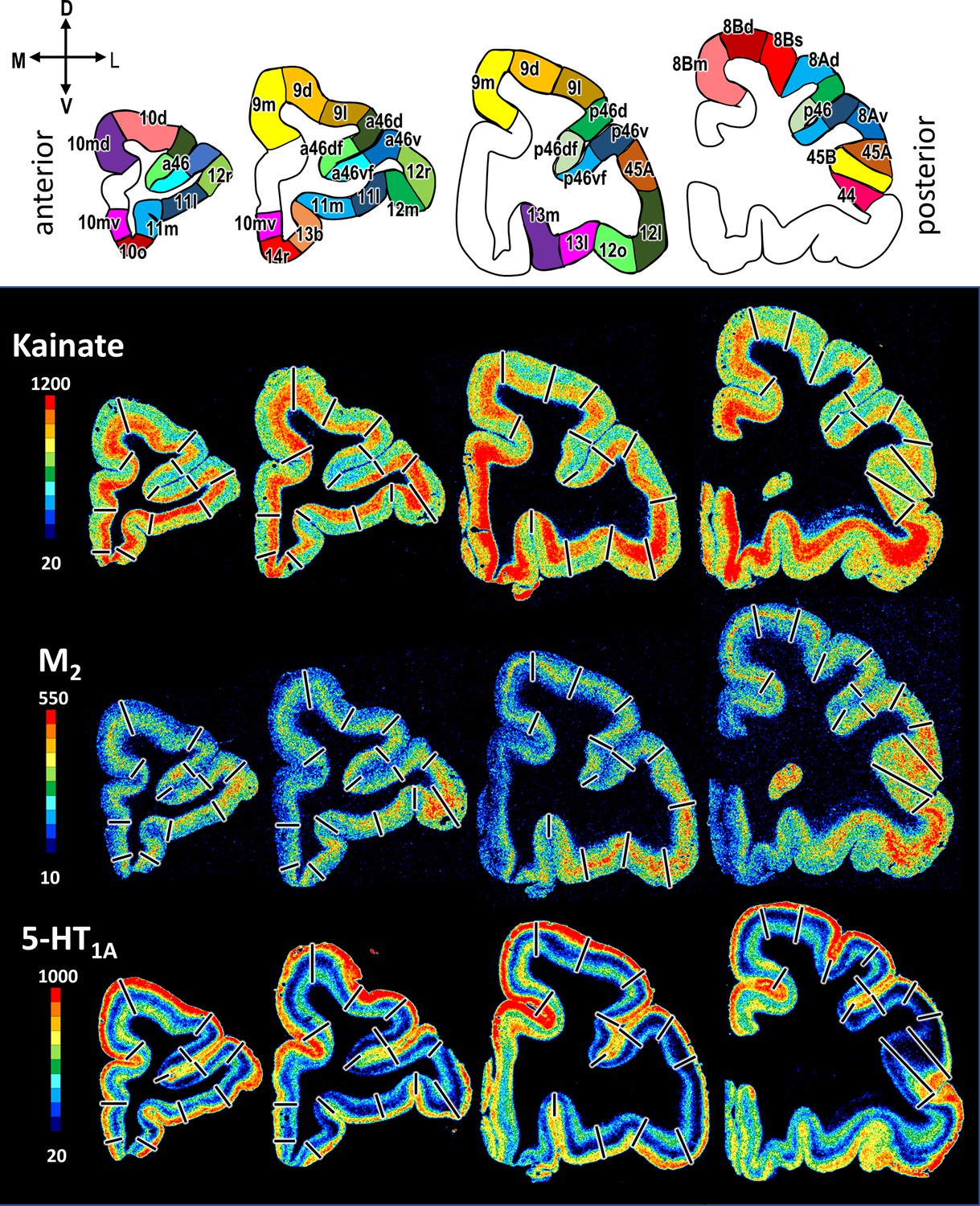
Exemplary sections depicting the distribution of kainate, M2 and 5-HT1A receptors in coronal sections through a macaque hemisphere.
The colour bar, positioned left to the autoradiographs, codes receptor densities in fmol/mg protein, and borders are indicated by black lines. The four schematic drawings at the top represent the distinct rostro-caudal levels and show the position of all prefrontal areas defined. C, caudal; D, dorsal; R, rostral; V, ventral.
Figure 9—figure supplement 1
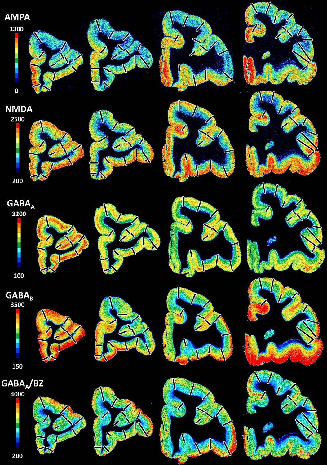
Exemplary sections depicting the distribution of the remaining receptor types, that is, of glutamate (AMPA, kainate, NMDA) and gamma-aminobutyric acid (GABA) (GABAA, GABAB, GABAA-associated benzodiazepine binding sites – BZ) receptors, in coronal sections through a macaque hemisphere.
The colour bar positioned left to the autoradiographs codes values of receptor densities in fmol/mg protein, and borders are indicated by the black lines.
Figure 9—figure supplement 2
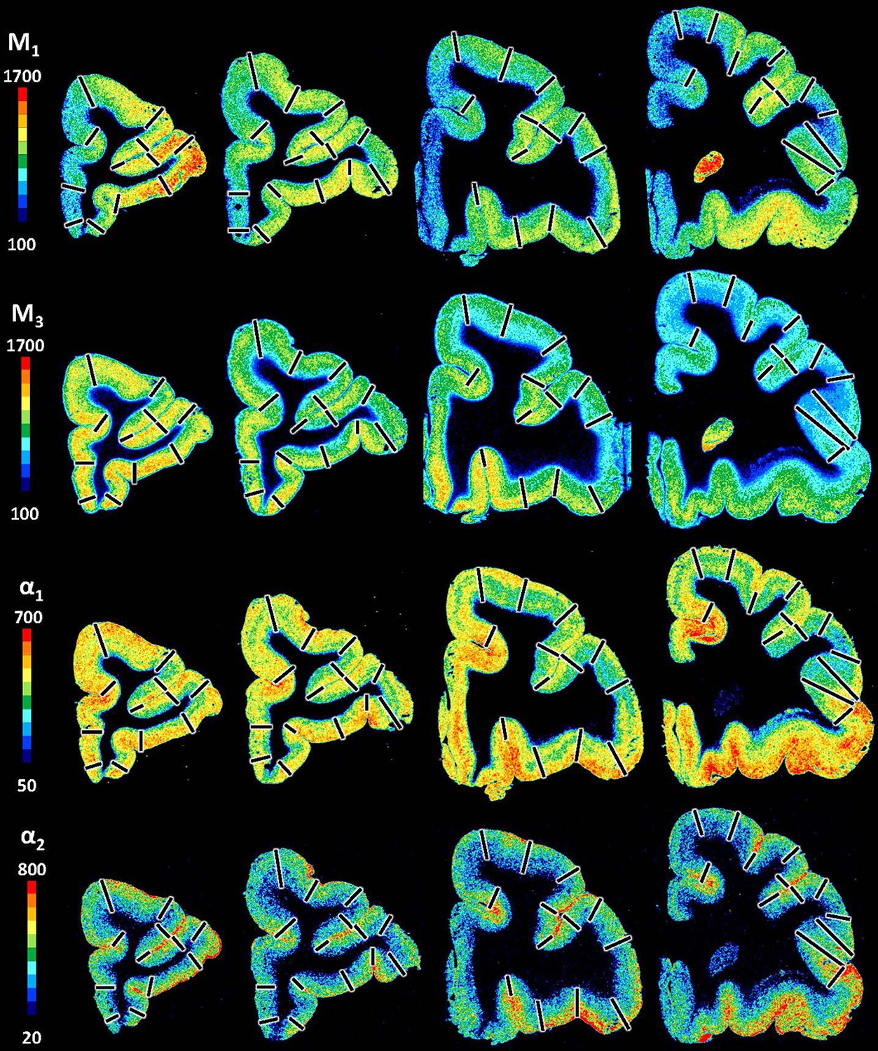
Exemplary sections depicting the distribution of the remaining receptor types, that is, acetylcholine (M1, M2, M3) and noradrenalin (α1, α2) receptors in coronal sections through a macaque hemisphere.
The colour bar positioned left to the autoradiographs codes values of receptor densities in fmol/mg protein, and borders are indicated by the black lines.
Figure 9—figure supplement 3

Exemplary sections depicting the distribution of the remaining receptor types, that is, serotonin (5HT2) and dopamine (D1) receptors in coronal sections through a macaque hemisphere.
The colour bar positioned left to the autoradiographs codes values of receptor densities in fmol/mg protein, and borders are indicated by the black lines.
Figure 10 with 1 supplement
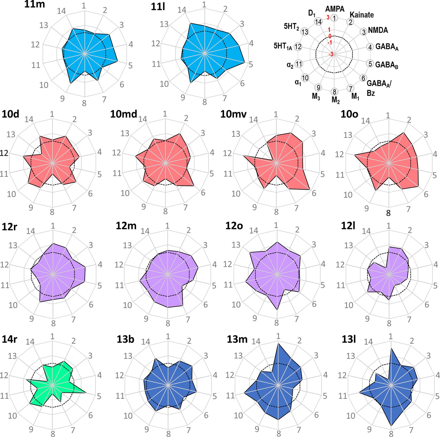
Normalized receptor fingerprints of the frontopolar and orbital areas.
Black dotted line on the plot represents the mean value over all areas for each receptor. Receptors displaying a negative z-score are indicative of absolute receptor densities which are lower than the average of that specific receptor over all examined areas. The opposite is true for positive z-scores. Labelling of different receptor types, as well as the axis scaling, is identical for each area plot, which is specified in the polar plot on the top of the figure.
Figure 10—figure supplement 1
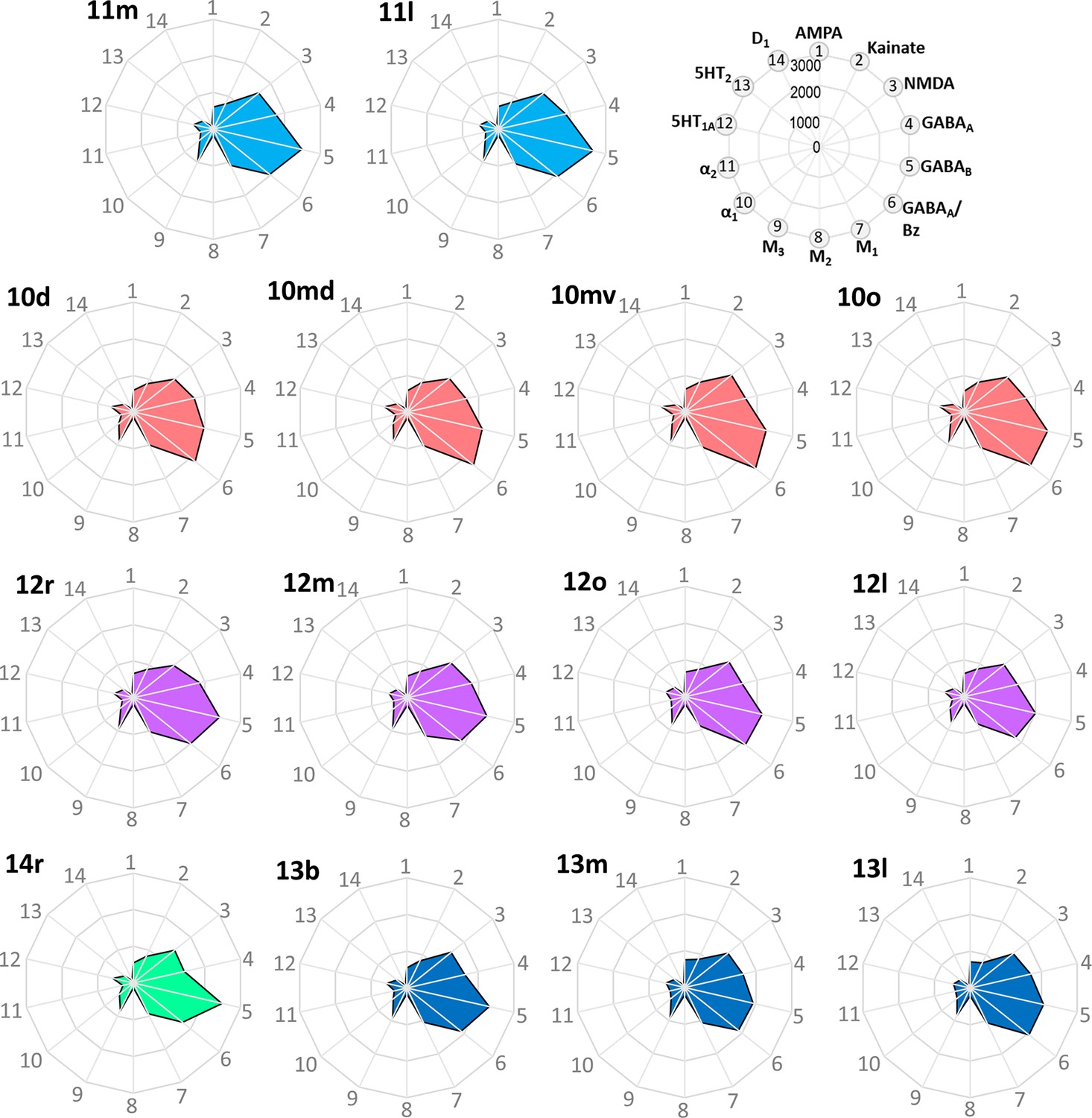
Receptor fingerprints of the frontopolar and orbital areas.
Absolute receptor densities are given in fmol/mg protein. The positions of the different receptor types and the axis scaling are identical in all areas, and specified in the polar plot on the top of the figure.
Figure 11 with 1 supplement
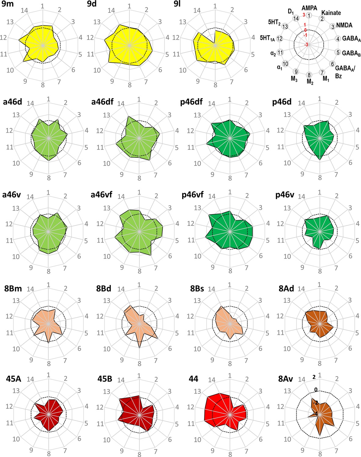
Normalized receptor fingerprints of the medial, dorsolateral, lateral, and ventrolateral areas.
Black dotted line on the plot represents the mean value over all areas for each receptor. Receptors displaying a negative z-score are indicative of absolute receptor densities which are lower than the average of that specific receptor over all examined areas. The opposite is true for positive z-scores. Labelling of different receptor types, as well as the axis scaling, is identical for each area plot, which is specified in the polar plot on the top of the figure. Due to the low receptor densities measured in area 8Av, scaling for its fingerprint is adjusted and shown directly on the corresponding polar plot.
Figure 11—figure supplement 1
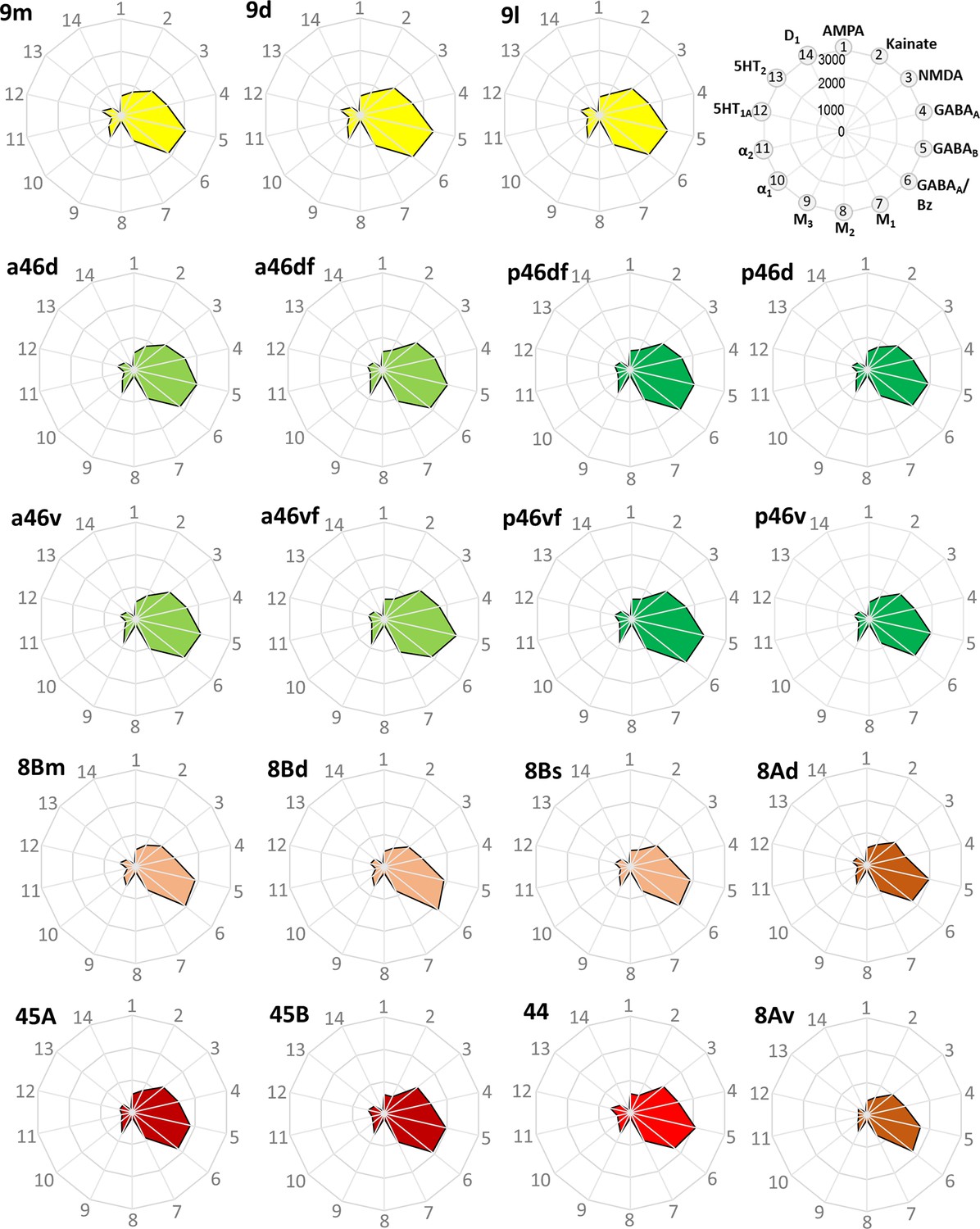
Receptor fingerprints of the medial, dorsolateral, lateral, and ventrolateral areas.
Absolute receptor densities are given in fmol/mg protein. The positions of the different receptor types and the axis scaling are identical in all areas, and specified in the polar plot on the top of the figure.
Figure 12
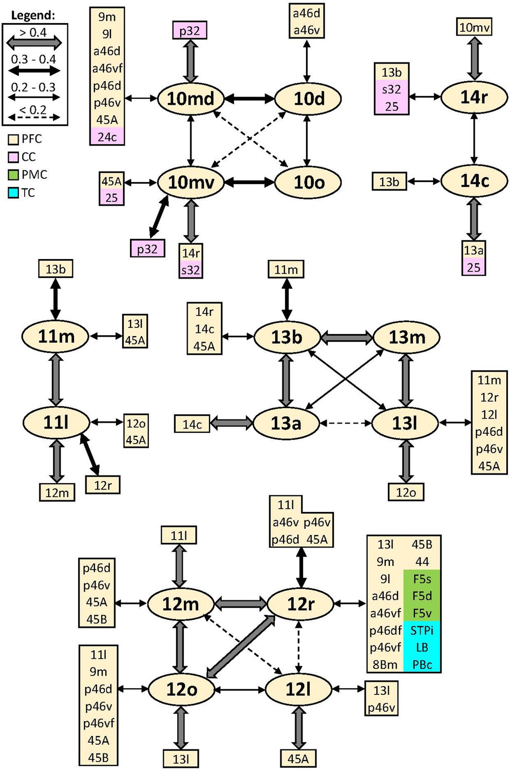
Schematic summary of the functional connectivity analysis between subdivisions of areas 10, 14, 11, 13, and 12.
Legend shows the strength of the functional connectivity coefficient (z) is coded by the appearance (wider-thinner-doted) of the connecting arrows. Areas related to different brain regions are marked on the scheme with distinct colours; prefrontal cortex (PFC) in light yellow, cingulate cortex (CC) in pink, premotor cortex (PMC) in light green, and temporal cortex (TC) in light blue.
Figure 13
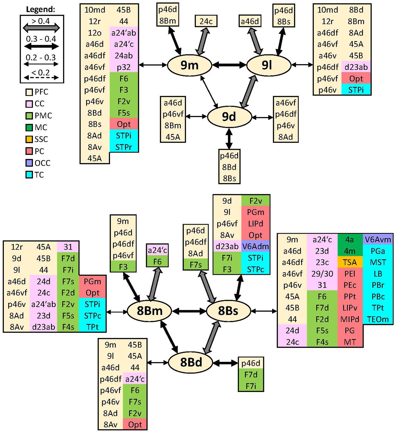
Schematic summary of the functional connectivity analysis between subdivisions of areas 9 and 8B.
Legend shows the strength of the functional connectivity coefficient (z) is coded by the appearance (wider-thinner-doted) of the connecting arrows. Areas related to different brain region are marked on the scheme with distinct colours; prefrontal cortex (PFC) in light yellow, cingulate cortex (CC) in pink, premotor cortex (PMC) in light green, motor cortex (MC) in dark green, somatosensory cortex (SSC) in orange, parietal cortex (PC) in red, occipital cortex (OCC) in purple, and temporal cortex (TC) in light blue.
Figure 14
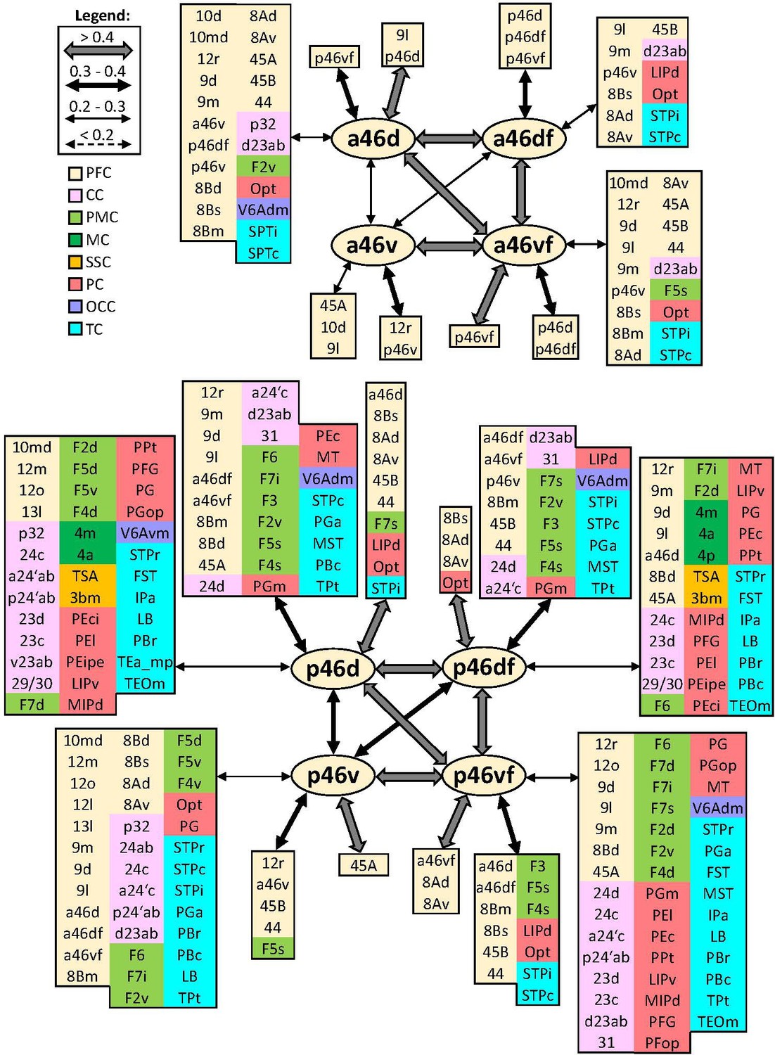
Schematic summary of the functional connectivity analysis between subdivisions of areas 46, rostral areas ‘a46,’ and caudal ones ‘p46’.
Legend shows the strength of the functional connectivity coefficient (z) is coded by the appearance (wider-thinner-doted) of the connecting arrows. Areas related to different brain region are marked on the scheme with distinct colours; prefrontal cortex (PFC) in light yellow, cingulate cortex (CC) in pink, premotor cortex (PMC) in light green, motor cortex (MC) in dark green, somatosensory cortex (SSC) in orange, parietal cortex (PC) in red, occipital cortex (OCC) in purple, and temporal cortex (TC) in light blue.
Figure 15
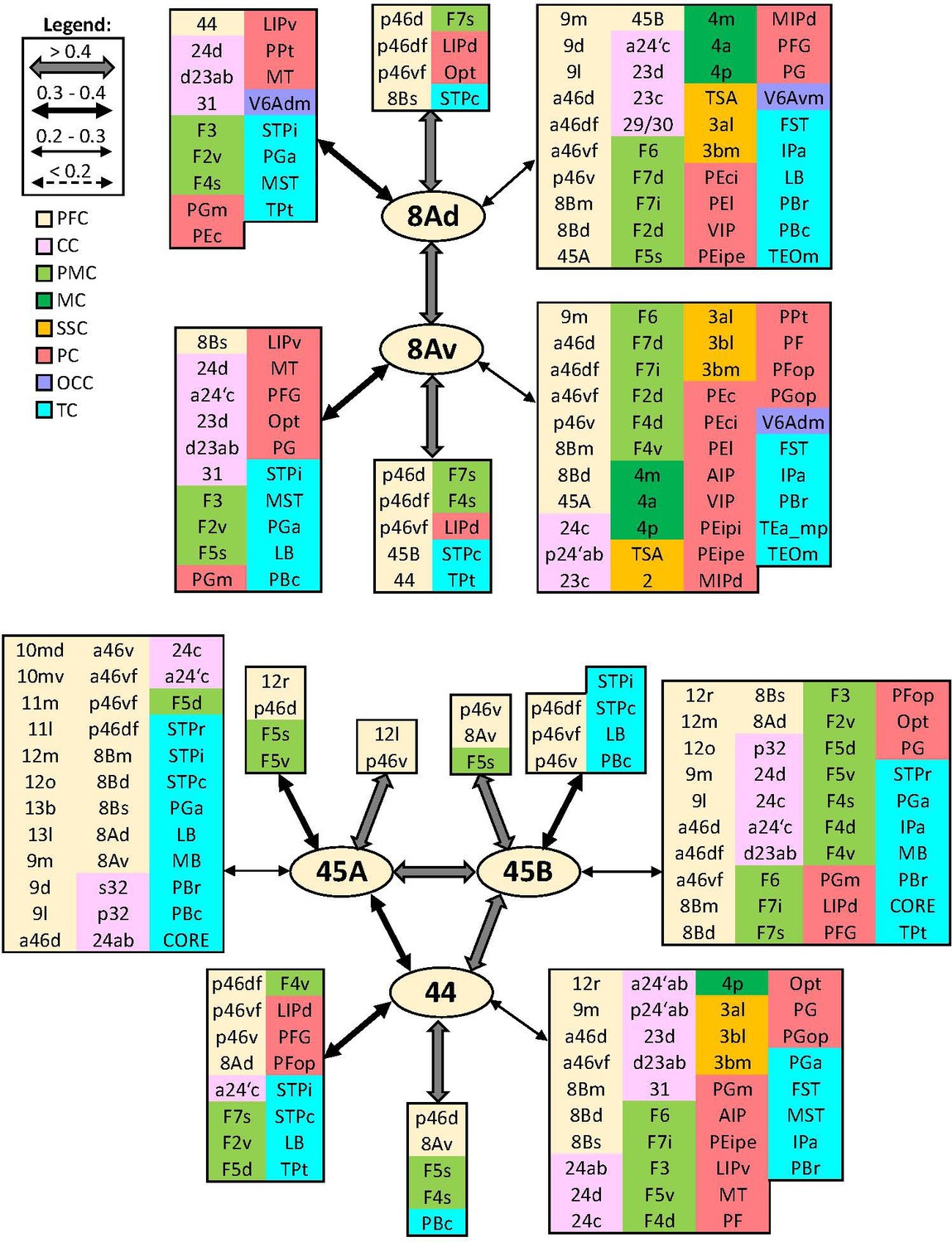
Schematic summary of the functional connectivity analysis between subdivisions of areas 8A and 45, and area 44.
Legend shows the strength of the functional connectivity coefficient (z) is coded by the appearance (wider-thinner-doted) of the connecting arrows. Areas related to different brain region are marked on the scheme with distinct colours; prefrontal cortex (PFC) in light yellow, cingulate cortex (CC) in pink, premotor cortex (PMC) in light green, motor cortex (MC) in dark green, somatosensory cortex (SSC) in orange, parietal cortex (PC) in red, occipital cortex (OCC) in purple, and temporal cortex (TC) in light blue.
Figure 16
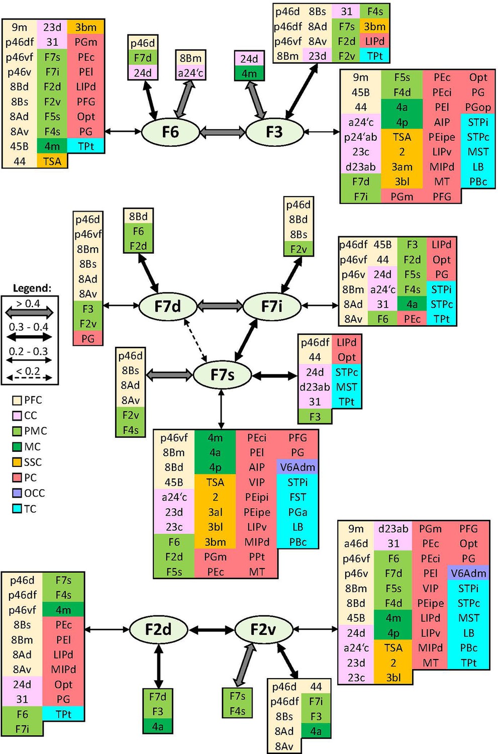
Schematic summary of the functional connectivity analysis between subdivisions of premotor areas F7 and F2, and areas F3 and F6.
Legend shows the strength of the functional connectivity coefficient (z) is coded by the appearance (wider-thinner-doted) of the connecting arrows. Areas related to different brain region are marked on the scheme with distinct colours; prefrontal cortex (PFC) in light yellow, cingulate cortex (CC) in pink, premotor cortex (PMC) in light green, motor cortex (MC) in dark green, somatosensory cortex (SSC) in orange, parietal cortex (PC) in red, occipital cortex (OCC) in purple, and temporal cortex (TC) in light blue.
Figure 17
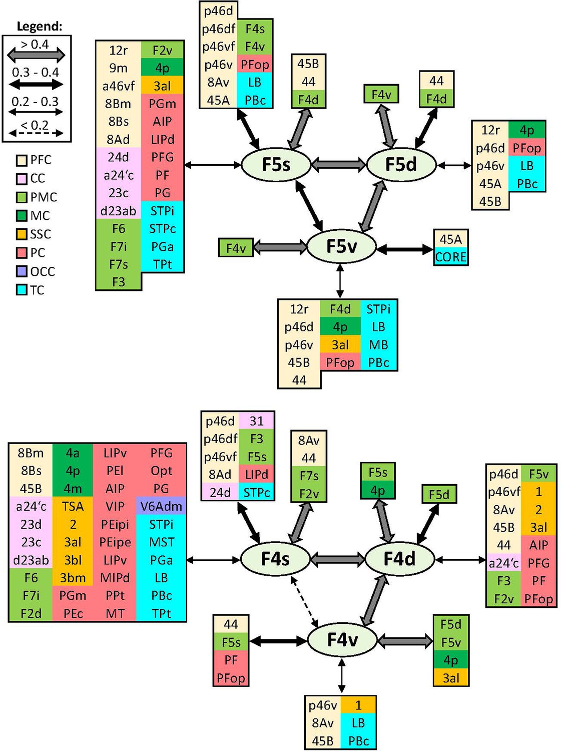
Schematic summary of the functional connectivity analysis between subdivisions of premotor areas F5 and F4.
Legend shows the strength of the functional connectivity coefficient (z) is coded by the appearance (wider-thinner-doted) of the connecting arrows. Areas related to different brain region are marked on the scheme with distinct colours; prefrontal cortex (PFC) in light yellow, cingulate cortex (CC) in pink, premotor cortex (PMC) in light green, motor cortex (MC) in dark green, somatosensory cortex (SSC) in orange, parietal cortex (PC) in red, occipital cortex (OCC) in purple, and temporal cortex (TC) in light blue.
Figure 18
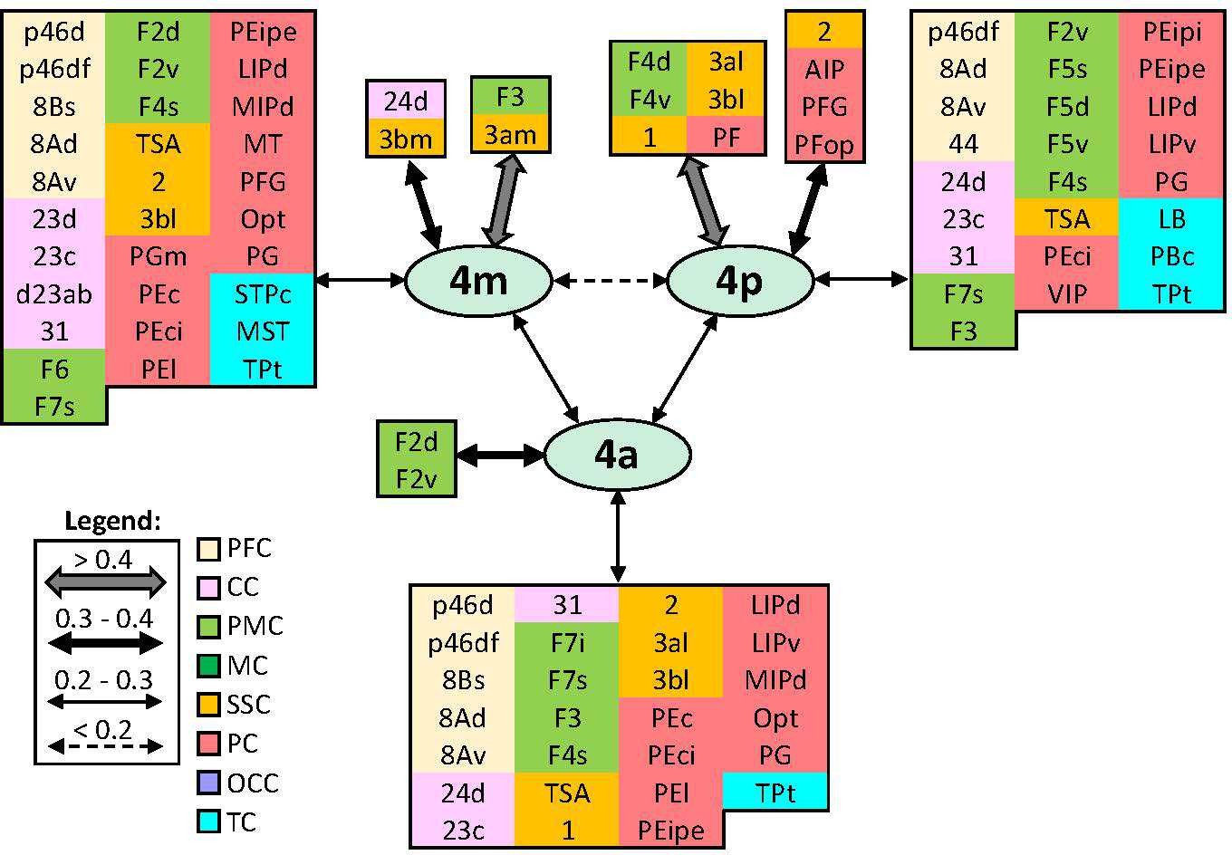
Schematic summary of the functional connectivity analysis between subdivisions of primary motor areas 4.
Legend shows the strength of the functional connectivity coefficient (z) is coded by the appearance (wider-thinner-doted) of the connecting arrows. Areas related to different brain region are marked on the scheme with distinct colours; prefrontal cortex (PFC) in light yellow, cingulate cortex (CC) in pink, premotor cortex (PMC) in light green, motor cortex (MC) in dark green, somatosensory cortex (SSC) in orange, parietal cortex (PC) in red, occipital cortex (OCC) in purple, and temporal cortex (TC) in light blue.
Figure 19
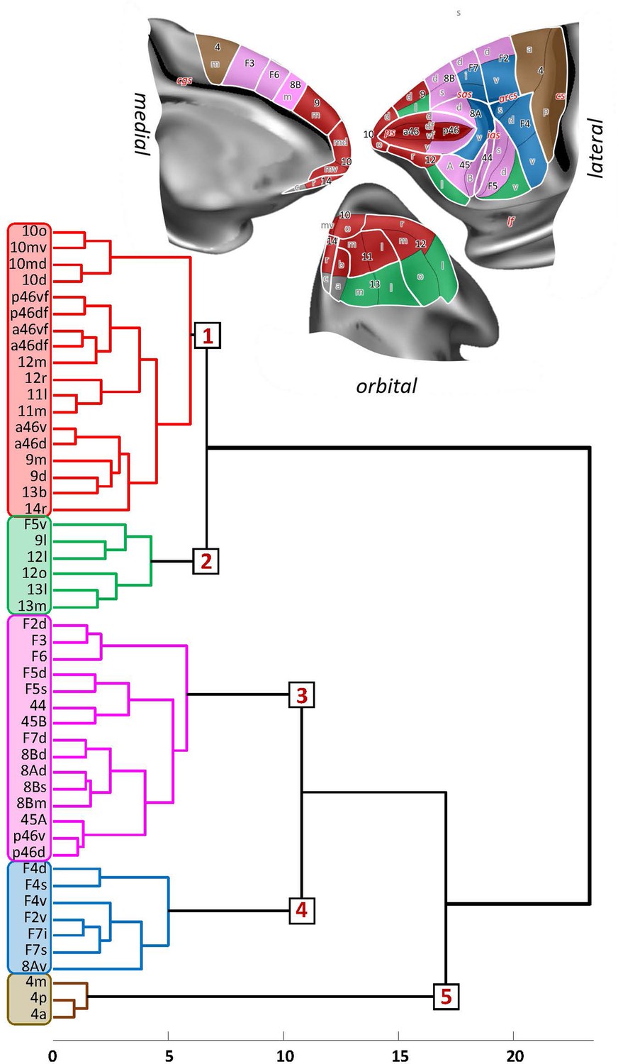
Receptor-driven hierarchical clustering of the receptor fingerprints in the macaque frontal lobe.
The analyses include 33 of the 35 areas identified in this study (for areas 14c and 13a was not possible to extract receptor densities due to technical limitations), as well as 16 areas of the primary motor and premotor cortex identified in a previous study (Rapan et al., 2021) carried out on the same monkey brains. Above the hierarchical dendrogram, the extent and location of the five clusters are depicted on the medial, lateral, and orbital surface of the Yerkes19 atlas. Clusters are colour coded based on the corresponding colour on the dendrogram.
Figure 20
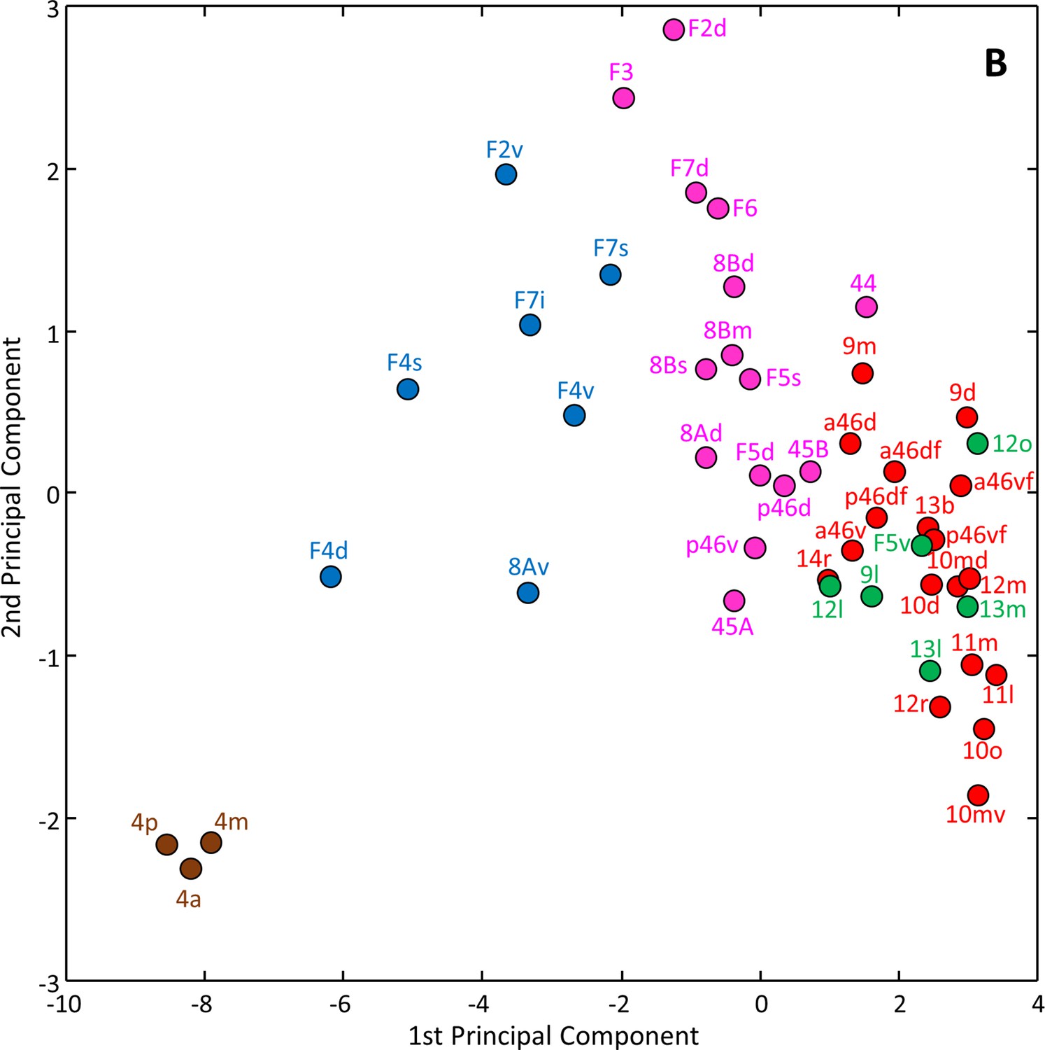
Principal component analysis (variance 79.8%) of the receptor fingerprints, where the k-means analysis showed five as the optimal number of clusters.
Author response image 1

Tables
Table 1
A list of cortical areas identified by the different authors (Walker, 1940; Petrides and Pandya, 1994; Petrides and Pandya, 2002; Preuss and Goldman-Rakic, 1991; Morecraft et al., 2012; Caminiti et al., 2017), whose maps were used as references for the present analysis, compared to areas identified by Rapan and colleagues.
‘a46’, areas a46d, a46df, a46vf, a46v; ‘p46’, areas p46d, p46df, p46vf, p46v; ‘p46d’, areas p46d, p46df; ‘p46v’, areas p46v, p46vf.
| Walker vs.Rapan | Preuss & Goldman-Rakic vs.Rapan | Carmichael & Price vs.Rapan | |||
|---|---|---|---|---|---|
| 10 | 10d | 10 | 10d | 10m | 10d |
| 10md | 10md | 10md | |||
| 10mv | 10mv | 10mv | |||
| 10o | 10o | 10o | 10o | ||
| Rostral part of 'a46', 11m, 14r, 13b | Rostral part of a46d and a46v | ||||
| 9 | 9d | 9d | 9d | n.a. | |
| 9l | 9l | ||||
| 9m | 9m | 9m | |||
| 8B | 8Bd | 8Bd | 8Bd | n.a. | |
| 8Bs | 8Bs | ||||
| 8Bm | 8Bm | 8Bm | |||
| Caudal part of 9d, 9l, and 9m | Caudal part of 9d, 9l, and 9m | ||||
| 8A | 8Ad | 8Ar | 8Ad, 8Av, 45A, caudal part of 'p46' | n.a. | |
| 8Av | 8Am | 8Ad | |||
| Caudal part of 'p46' | 8Ac | 8Av | |||
| 46 | a46' | 46r | a46df, a46vf | n.a. | |
| p46' | 46dr | a46d, p46d, ventral part of 9l | |||
| Dorsal part of 12r; ventral part of 9l | 46vr | a46v, p46v, dorsal part of 12r | |||
| Rostroventral part of 8Ad; rostrodorsal part of 45A | 46d | a46df, p46df | |||
| 46v | a46vf, p46vf | ||||
| 45 | 45A | 45 | 45B, 44 | n.a. | |
| 45B | |||||
| Rostroventral part of 8Av | |||||
| n.a. | n.a. | n.a. | |||
| 12 | 12r | 12vl | 12r | 12r | 12r |
| 12m | 12l | 12m | 12m, 12o | ||
| 12l | Rostral part of 45A | 12l | 12l | ||
| 12o | 12o | 12o | |||
| Part of 45A; 13l | |||||
| 13 | 13m | 13M | 13m | 13b | 13b |
| 13l | 13L | 13l | 13a | 13a | |
| 13m | 13m | ||||
| 13l | 13l | ||||
| 11 | 11m | 11 | 11m | 11m | 11m |
| 11l | 11l | 11l | 11l | ||
| Part of12m, ventral part of 12l | |||||
| 14 | 14r | 14A | 14r, 10o, 10mv, 11m, 13b | 14r | 14r |
| 14c | 14M | 14r, 14c | 14c | 14c | |
| Part of 11m; 13b, 13a | 14L | 14r, 14c, 13b, 13a | |||
| Petrides & Pandya vs.Rapan | Morecraft vs.Rapan | Caminiti vs.Rapan | |||
| 10 | 10d | 10 | 10d | 10 | 10d |
| 10md | 10md | 10md | |||
| 10mv | 10mv | 10mv | |||
| 10o | 10o | 10o | |||
| Rostral part of a46d and a46v; ventral part of 12r | Rostral part of a46d and a46v | Rostral part of a46d and a46v | |||
| 9 | 9d | 9 | 9d | 9l | 9d |
| 9l | 9l | 9l | |||
| 9m | 9m | 9m | 9m | 9m | |
| 8B | 8Bd | 8Bd | 8Bd | 8B | 8Bd |
| 8Bs | 8Bs | 8Bs | |||
| 8Bm | 8Bm | 8Bm | 8Bm | ||
| Caudal part of 9d, 9l, and 9m | Caudal part of 9d, 9l, and 9m | Caudal part of 9d, 9l, and 9m | |||
| 8Ad | 8Ad | 8Ad | 8Ad | 8Ad | 8Ad |
| 8Av | 8Av | 8Av | 8Av | 8Av | 8Av |
| Caudal part of 'p46' | Caudal part of 'p46' | Caudal part of 'p46' | |||
| 46 | a46' | 46 | a46' | 46dr | a46d, a46df |
| 9/46d | p46d' | 9/46d | p46d' | 46vr | a46v, a46vf |
| 9/46v | p46v' | 9/46v | p46v' | 46dc | Caudal part of a46d and a46df, 'p46d' |
| r46vc | Caudal part of 'a46v', rostral part of 'p46v' | ||||
| c46vc | p46v, p46vf | ||||
| 45A | 45A | 45 | 45A | 45A | 45A |
| 45B | 45B | 45B | 45B | ||
| 44 | 44 | 44 | 44, F5s | n.a. | |
| 47/12 | 12r | 47/12 | 12r | r12r | 12r |
| 12l | 12l | i12r | 12r | ||
| 12m | c12r | 12r, rostral part of 12l and 45A | |||
| 12o | 12l | 12l | |||
| 12m | 12m, 12o | ||||
| 12o | 12o | ||||
| 13 | 13m | n.a. | 13a/13b | 13a, 13b | |
| 13l | 13m/13l | 13m, 13l | |||
| 11 | 11l, part of 12r and 12m | n.a. | 11m | 11m | |
| 11l | 11l, 11m | ||||
| 14 | 14r | 14 | 14r | 14 | 14r |
| 14c | 14c | 14c | |||
| Caudal part of 10mv; 13a, 13b | Caudal part of 10mv | 10mv | |||
Table 2
Prominent cytoarchitectonic features highlighted for all 35 identified prefrontal areas.
| Area | Layer IV | Cytoarchitecture | |
|---|---|---|---|
| 10d | Granular | Small-size pyramids in III/V; dense granular layers II/IV | |
| 10md | Wide, pale layer V | ||
| 10mv | Prominent middle-size pyramids in V | ||
| 10o | Prominent layer II | ||
| 14r | Dysgranular | well-developed layer II; columnar pattern in IV-V | |
| 14c | Agranular | Pale layer III | |
| 11m | Granular | Sublamination of V (Va/Vb); cell clusters in Va | |
| 11l | Sublamination of V (Va/Vb) | ||
| 13b | Granular | Columnar pattern in IV-V | |
| 13a | Dysgranular | Sublamination of V (Va/Vb) | |
| 13m | Sublamination of V (Va/Vb); layer Va wider than Vb | ||
| 13l | Sublamination of V (Va/Vb); both layers of comparable width | ||
| 12r | Dysgranular | No sublamination of V | |
| 12m | Granular | Sublamination of V (Va/Vb) | |
| 12l | Sublamination of V (Va/Vb) | ||
| 12o | Dysgranula | No sublamination of V | |
| 9m | Granular | Sublamination of V (Va/Vb) | |
| 9d | Gradient in cell-size within III; sublamination of V (Va/Vb); pale layer Vb is wider in 9d than 9l | ||
| 9l | Gradient in cell size within III; sublamination of V (Va/Vb) | ||
| a46d | Granular | Scattered middle-sized pyramids in upper layer V | Well-developed layer II |
| a46df | Scattered middle-sized pyramids in lower layer III | ||
| a46vf | Scattered middle-sized pyramids in layer III | ||
| a46v | Prominent layer II, but not as in a46d | ||
| p46d | Granular | Cells more uniform in size throughout the cortex | Well-developed layer II; densely packed cells in layer III |
| p46df | Densely packed cells in layer III; scattered middle-sized pyramids in lower layer III | ||
| p46vf | Scattered middle-sized pyramids in layer III | ||
| p46v | Prominent layer II, but not as in p46d | ||
| 8Bm | Dysgranular | Layer VI pale compared to dorsal subdivisions | |
| 8Bd | Dark, prominent layer II | ||
| 8Bs | Small size pyramids in III and V compared to 8Bd | ||
| 8Ad | Granular | Upper layer III pale | |
| 8Av | Lower layer III pale; highly granular cortex | ||
| 45A | Granular | Middle-sized pyramids in layer III | |
| 45B | Layer IV less developed | ||
| 44 | Dysgranular | Few larger pyramids scattered in layer V | |
Table 3
Absolute receptor densities (mean ± SD) in fmol/mg protein.
BZ, GABAA-associated benzodiazepine binding sites.
| Area | AMPA | Kainate | NMDA | GABAA | GABAB | BZ | M1 | M2 | M3 | α1 | α2 | 5-HT1A | 5-HT2 | D1 |
|---|---|---|---|---|---|---|---|---|---|---|---|---|---|---|
| 10d SD | 591 161 | 858 116 | 1430 260 | 1697 162 | 1970 542 | 2151 829 | 995 230 | 141 35 | 880 117 | 507 75 | 337 68 | 623 169 | 340 75 | 93 20 |
| 10md SD | 586 106 | 895 90 | 1470 177 | 1651 168 | 2095 495 | 2307 783 | 1012 274 | 154 45 | 856 112 | 494 48 | 327 48 | 628 151 | 357 60 | 90 20 |
| 10mv SD | 628 130 | 903 66 | 1612 151 | 1680 199 | 2254 606 | 2451 839 | 1063 332 | 145 35 | 894 124 | 471 94 | 334 56 | 666 214 | 320 67 | 86 18 |
| 10o SD | 569 76 | 909 50 | 1523 190 | 1723 160 | 2336 612 | 2327 774 | 1068 313 | 150 45 | 923 105 | 470 76 | 342 76 | 682 233 | 350 59 | 82 12 |
| 14r SD | 470 81 | 818 107 | 1442 255 | 1427 162 | 2482 424 | 1715 542 | 921 385 | 134 35 | 833 118 | 497 109 | 297 95 | 583 119 | 323 44 | 86 15 |
| 11m SD | 604 100 | 771 65 | 1585 139 | 1762 142 | 2476 466 | 1975 218 | 1094 200 | 159 64 | 965 132 | 473 50 | 342 40 | 549 167 | 357 60 | 92 27 |
| 11l SD | 623 111 | 807 123 | 1562 113 | 1876 235 | 2644 478 | 2066 247 | 1050 228 | 159 54 | 944 101 | 462 46 | 351 45 | 529 116 | 357 51 | 96 29 |
| 13b SD | 489 44 | 820 103 | 1548 223 | 1615 120 | 2311 452 | 1901 431 | 1039 263 | 166 57 | 897 104 | 480 73 | 350 75 | 562 206 | 355 57 | 93 22 |
| 13m SD | 753 67 | 856 111 | 1499 122 | 1622 126 | 1908 429 | 1864 269 | 1059 121 | 206 94 | 918 130 | 485 21 | 417 21 | 527 138 | 357 50 | 78 11 |
| 13l SD | 713 95 | 756 60 | 1498 187 | 1683 180 | 2057 240 | 2052 303 | 1054 148 | 223 78 | 826 108 | 461 15 | 404 26 | 460 107 | 351 43 | 70 4 |
| 12r SD | 659 122 | 854 120 | 1406 121 | 1843 283 | 2412 312 | 1991 307 | 1026 301 | 180 72 | 922 96 | 439 38 | 306 52 | 540 88 | 350 51 | 86 9 |
| 12m SD | 598 136 | 799 55 | 1533 175 | 1792 246 | 2222 353 | 1873 421 | 1152 262 | 202 74 | 918 108 | 481 48 | 379 71 | 504 103 | 354 45 | 86 22 |
| 12l SD | 630 112 | 840 73 | 1400 126 | 1494 221 | 2010 483 | 1789 417 | 824 347 | 182 75 | 780 132 | 491 82 | 320 43 | 531 163 | 351 48 | 71 6 |
| 12o SD | 670 165 | 817 97 | 1527 158 | 1579 267 | 2142 414 | 2102 436 | 888 174 | 209 64 | 832 149 | 484 32 | 401 66 | 541 87 | 384 61 | 89 20 |
| 9m SD | 607 125 | 818 84 | 1224 252 | 1460 352 | 2048 235 | 1864 449 | 868 196 | 168 33 | 760 79 | 508 50 | 307 49 | 629 136 | 359 55 | 89 22 |
| 9d SD | 584 154 | 766 72 | 1341 206 | 1633 338 | 2312 235 | 2081 478 | 1050 177 | 176 34 | 841 80 | 515 40 | 355 59 | 642 81 | 362 61 | 92 24 |
| 9l SD | 554 151 | 711 56 | 1311 230 | 1582 324 | 2173 260 | 1972 464 | 1029 143 | 164 31 | 822 91 | 497 38 | 361 47 | 594 64 | 366 54 | 67 21 |
| a46d SD | 527 138 | 810 81 | 1247 197 | 1609 253 | 1993 189 | 1821 349 | 981 234 | 187 40 | 819 114 | 462 68 | 318 65 | 521 86 | 354 66 | 90 26 |
| a46df SD | 559 126 | 667 44 | 1348 124 | 1663 219 | 2071 170 | 1898 444 | 1083 160 | 176 45 | 860 79 | 478 60 | 384 61 | 466 94 | 355 80 | 94 29 |
| a46vf SD | 619 126 | 679 81 | 1427 102 | 1752 297 | 2291 280 | 1873 352 | 1124 161 | 180 47 | 894 94 | 484 47 | 395 39 | 497 88 | 376 76 | 93 30 |
| a46v SD | 502 67 | 808 61 | 1339 167 | 1614 281 | 2068 200 | 1908 406 | 1017 235 | 187 52 | 856 85 | 440 52 | 319 35 | 496 79 | 349 58 | 87 17 |
| p46d SD | 563 103 | 785 50 | 1187 318 | 1449 259 | 1934 231 | 1786 286 | 889 257 | 185 48 | 771 84 | 439 70 | 300 30 | 484 77 | 364 35 | 81 29 |
| p46df SD | 592 102 | 692 40 | 1305 254 | 1649 268 | 2049 177 | 1978 256 | 1000 241 | 176 43 | 812 84 | 453 78 | 388 47 | 478 86 | 373 42 | 85 22 |
| p46vf SD | 613 115 | 671 71 | 1369 225 | 1726 315 | 2295 315 | 2138 383 | 998 230 | 163 41 | 834 115 | 467 74 | 395 67 | 528 107 | 381 48 | 88 24 |
| p46v SD | 519 49 | 758 67 | 1241 207 | 1444 279 | 1956 213 | 1814 284 | 810 294 | 170 34 | 783 74 | 416 88 | 321 43 | 461 98 | 361 43 | 81 23 |
| 8Bm SD | 528 136 | 731 128 | 1018 438 | 1216 217 | 1888 267 | 1958 236 | 806 173 | 178 31 | 667 87 | 472 70 | 273 49 | 508 80 | 351 32 | 83 27 |
| 8Bd SD | 481 92 | 641 106 | 973 346 | 1195 151 | 1896 173 | 2136 385 | 832 131 | 195 41 | 680 92 | 466 73 | 263 70 | 437 89 | 362 47 | 89 28 |
| 8Bs SD | 494 99 | 570 54 | 1047 348 | 1232 209 | 1901 389 | 1931 134 | 831 117 | 164 47 | 682 117 | 436 75 | 304 67 | 484 106 | 356 56 | 88 23 |
| 8Ad SD | 528 115 | 694 65 | 1108 322 | 1219 200 | 1972 143 | 1795 301 | 870 227 | 158 37 | 685 139 | 438 67 | 272 36 | 450 82 | 359 43 | 82 29 |
| 8Av SD | 440 94 | 591 102 | 1017 264 | 1205 202 | 1703 264 | 1807 369 | 708 268 | 163 36 | 603 174 | 347 112 | 257 64 | 262 109 | 323 67 | 79 25 |
| 45A SD | 550 97 | 733 61 | 1235 165 | 1461 186 | 1846 280 | 1810 378 | 880 244 | 168 52 | 734 62 | 422 106 | 321 47 | 394 126 | 358 47 | 75 19 |
| 45B SD | 601 150 | 588 54 | 1310 271 | 1472 286 | 1955 301 | 1911 249 | 972 317 | 147 29 | 705 120 | 442 65 | 372 75 | 499 166 | 378 58 | 88 30 |
| 44 SD | 595 162 | 592 86 | 1310 277 | 1520 220 | 2065 233 | 1756 294 | 957 339 | 154 22 | 697 164 | 475 79 | 402 70 | 638 253 | 385 57 | 93 27 |
Table 4
FDR-corrected p-values for the post hoc tests (i.e. third-level tests; p-values were corrected for 258 comparisons per receptor type).
No p-values are provided for the M1, M2, 5-HT2, or D1 receptors because they did not reach the level of significance in the second-level test. Green background highlights significant pairs of adjacent prefrontal areas in the macaque brain. *p<0.05, **p<0.01, ***p<0.001.
| AMPA | Kainate | NMDA | GABAᴀ | GABAB | BZ | M3 | α1 | α2 | 5-HT1A | |
|---|---|---|---|---|---|---|---|---|---|---|
| 10d - 10md | 0.9393 | 0.5591 | 0.8028 | 0.8776 | 0.6976 | 0.7871 | 0.7553 | 0.9104 | 0.866 | 0.9753 |
| 10d - 9d | 0.9041 | 0.1142 | 0.5721 | 0.8364 | 0.1413 | 0.8728 | 0.6135 | 0.9104 | 0.5692 | 0.9081 |
| 10d - 9l | 0.618 | 0.0091** | 0.4329 | 0.5871 | 0.4474 | 0.7277 | 0.4173 | 0.9549 | 0.4603 | 0.746 |
| 10d - a46d | 0.3472 | 0.4435 | 0.194 | 0.7085 | 0.9711 | 0.3149 | 0.3845 | 0.5571 | 0.6929 | 0.1842 |
| 10md - 10mv | 0.6304 | 0.8867 | 0.3033 | 0.9407 | 0.4908 | 0.8415 | 0.586 | 0.7554 | 0.8435 | 0.7195 |
| 10md - 9m | 0.8231 | 0.1508 | 0.0461* | 0.1826 | 0.8701 | 0.1242 | 0.1456 | 0.8313 | 0.5417 | 0.9816 |
| 10mv - 10o | 0.4391 | 0.9801 | 0.5458 | 0.8064 | 0.7872 | 0.8587 | 0.7441 | 0.9973 | 0.8276 | 0.9081 |
| 10mv - 14r | 0.0386* | 0.149 | 0.2167 | 0.1305 | 0.3529 | 0.0291* | 0.3522 | 0.7752 | 0.2444 | 0.3143 |
| 10o - 11m | 0.7018 | 0.0056** | 0.6676 | 0.8425 | 0.5291 | 0.2996 | 0.5396 | 0.9549 | 0.9936 | 0.0666 |
| 10o - 14r | 0.168 | 0.1227 | 0.5525 | 0.0366* | 0.5751 | 0.0291* | 0.1793 | 0.7645 | 0.1471 | 0.2115 |
| 11l - 11m | 0.8207 | 0.5126 | 0.8931 | 0.4519 | 0.4832 | 0.8721 | 0.7807 | 0.9104 | 0.7881 | 0.8618 |
| 11l - 12m | 0.8207 | 0.9666 | 0.9271 | 0.7045 | 0.058 | 0.7409 | 0.7964 | 0.8085 | 0.3854 | 0.8686 |
| 11l - 12r | 0.5848 | 0.3727 | 0.2291 | 0.8932 | 0.2739 | 0.8721 | 0.7446 | 0.7645 | 0.1325 | 0.917 |
| 11l - 13l | 0.2408 | 0.6732 | 0.9223 | 0.4866 | 0.0523 | 0.9766 | 0.2814 | 0.9549 | 0.1427 | 0.7352 |
| 11l - 13m | 0.1005 | 0.4105 | 0.9256 | 0.3035 | 0.0104* | 0.8678 | 0.9487 | 0.7645 | 0.0781 | 0.9081 |
| 11m - 13b | 0.0988 | 0.3998 | 0.8028 | 0.3063 | 0.4593 | 0.8728 | 0.2991 | 0.9549 | 0.8403 | 0.917 |
| 11m - 13l | 0.1593 | 0.9801 | 0.8261 | 0.8911 | 0.208 | 0.8652 | 0.19 | 0.9795 | 0.0925 | 0.6198 |
| 11m - 13m | 0.06 | 0.1684 | 0.8261 | 0.698 | 0.0554 | 0.9766 | 0.7943 | 0.8541 | 0.0465* | 0.997 |
| 11m - 14r | 0.0688 | 0.4928 | 0.2895 | 0.0159* | 0.9809 | 0.489 | 0.0347* | 0.812 | 0.149 | 0.8153 |
| 12l - 12o | 0.7396 | 0.7221 | 0.5477 | 0.7785 | 0.7117 | 0.5449 | 0.591 | 0.9338 | 0.0323* | 0.9837 |
| 12l - 12r | 0.7423 | 0.84 | 0.9808 | 0.0261* | 0.0824 | 0.7523 | 0.0613 | 0.3864 | 0.6495 | 0.9869 |
| 12l - 45A | 0.2779 | 0.0773 | 0.2152 | 0.8729 | 0.4924 | 0.9984 | 0.5606 | 0.148 | 0.9231 | 0.0933 |
| 12m - 12o | 0.4391 | 0.8664 | 0.9223 | 0.1851 | 0.7851 | 0.7313 | 0.2335 | 0.9973 | 0.6306 | 0.7877 |
| 12m - 12r | 0.4191 | 0.3735 | 0.3465 | 0.8326 | 0.4936 | 0.8721 | 0.9602 | 0.5104 | 0.0176* | 0.7772 |
| 12m - 13l | 0.1742 | 0.7207 | 0.9867 | 0.7785 | 0.7649 | 0.7496 | 0.4295 | 0.929 | 0.5069 | 0.8618 |
| 12o - 12r | 0.9669 | 0.5144 | 0.4782 | 0.0923 | 0.2583 | 0.8587 | 0.2335 | 0.5575 | 0.004** | 0.9881 |
| 12o - 13l | 0.5736 | 0.6021 | 0.9649 | 0.5306 | 0.9429 | 0.9901 | 0.9049 | 0.929 | 0.8128 | 0.6789 |
| 12r - a46v | 0.0151* | 0.3743 | 0.6393 | 0.0962 | 0.0824 | 0.8738 | 0.3415 | 0.9973 | 0.7023 | 0.6442 |
| 12r - p46v | 0.0427* | 0.0659 | 0.2246 | 0.0032** | 0.019* | 0.7409 | 0.0347* | 0.7253 | 0.6634 | 0.3438 |
| 13b - 14r | 0.8536 | 0.973 | 0.4654 | 0.2172 | 0.4936 | 0.7277 | 0.339 | 0.88 | 0.1052 | 0.9081 |
| 13l - 13m | 0.7624 | 0.2909 | 0.9979 | 0.8563 | 0.7452 | 0.8587 | 0.4298 | 0.8565 | 0.8354 | 0.6937 |
| 44A - 45B | 0.9416 | 0.9648 | 0.9808 | 0.8425 | 0.677 | 0.8415 | 0.933 | 0.6727 | 0.4447 | 0.089 |
| 45A - 45B | 0.5714 | 0.0122* | 0.6278 | 0.97 | 0.7593 | 0.8721 | 0.7363 | 0.7902 | 0.1275 | 0.2574 |
| 45A - 8Av | 0.0988 | 0.0062** | 0.095 | 0.1219 | 0.5291 | 0.9928 | 0.0476* | 0.0857 | 0.0401 | 0.0853 |
| 45A - p46v | 0.7274 | 0.6956 | 0.9363 | 0.9604 | 0.6792 | 0.9901 | 0.4861 | 0.9549 | 0.9686 | 0.4794 |
| 45B - 8Av | 0.0335* | 0.9801 | 0.0327* | 0.0914 | 0.3129 | 0.8721 | 0.1754 | 0.0238* | 0.0004*** | 0.0016** |
| 8Ad - 8Av | 0.2009 | 0.0487* | 0.5458 | 0.9852 | 0.1933 | 0.9897 | 0.2412 | 0.0155* | 0.6929 | 0.0073** |
| 8Ad - 8Bs | 0.7142 | 0.0183* | 0.7149 | 0.9407 | 0.8209 | 0.7836 | 0.9833 | 0.9978 | 0.2807 | 0.7062 |
| 8Ad - p46d | 0.6185 | 0.0705 | 0.5546 | 0.123 | 0.9152 | 0.9984 | 0.2024 | 0.9795 | 0.358 | 0.7062 |
| 8Av - p46v | 0.2667 | 0.0009*** | 0.0726 | 0.1047 | 0.2099 | 0.9915 | 0.0036** | 0.1038 | 0.0344* | 0.0043** |
| 8Bd - 8Bm | 0.6165 | 0.1226 | 0.7936 | 0.9194 | 0.9698 | 0.7409 | 0.9038 | 0.937 | 0.8403 | 0.4665 |
| 8Bd - 8Bs | 0.8684 | 0.2213 | 0.6066 | 0.8663 | 0.968 | 0.7386 | 0.9602 | 0.7048 | 0.2297 | 0.6243 |
| 8Bd - 9d | 0.1213 | 0.0168* | 0.0031** | 0.0011** | 0.0469* | 0.9557 | 0.0155* | 0.3477 | 0.0044** | 0.004** |
| 8Bm - 9m | 0.2744 | 0.1202 | 0.1303 | 0.115 | 0.5171 | 0.9071 | 0.1863 | 0.5663 | 0.2868 | 0.1364 |
| 8Bs - 9l | 0.385 | 0.0058** | 0.0364* | 0.0083** | 0.2099 | 0.9766 | 0.0362* | 0.1957 | 0.084 | 0.1598 |
| 9d - 9l | 0.6967 | 0.3221 | 0.8516 | 0.7657 | 0.5923 | 0.8587 | 0.7964 | 0.8085 | 0.8602 | 0.6144 |
| 9d - 9m | 0.7704 | 0.3551 | 0.3881 | 0.2172 | 0.2099 | 0.6636 | 0.2048 | 0.9384 | 0.1121 | 0.9095 |
| 9l - a46d | 0.7246 | 0.054 | 0.6553 | 0.8908 | 0.4226 | 0.7544 | 0.9602 | 0.5726 | 0.1595 | 0.3769 |
| a46df - a46d | 0.6801 | 0.004** | 0.4699 | 0.7705 | 0.7808 | 0.8728 | 0.5621 | 0.833 | 0.0257* | 0.5572 |
| a46df - a46vf | 0.3688 | 0.8465 | 0.5764 | 0.5843 | 0.3129 | 0.9857 | 0.6279 | 0.9549 | 0.747 | 0.7573 |
| a46df-p46df | 0.6714 | 0.6574 | 0.7815 | 0.9612 | 0.9519 | 0.8721 | 0.528 | 0.6964 | 0.9208 | 0.9138 |
| a46d-p46d | 0.6434 | 0.6648 | 0.6831 | 0.3038 | 0.8504 | 0.9781 | 0.5283 | 0.7053 | 0.5933 | 0.7062 |
| a46vf - a46v | 0.0688 | 0.0105* | 0.5349 | 0.3464 | 0.3066 | 0.9766 | 0.5895 | 0.4481 | 0.0101* | 0.9936 |
| a46vf - p46vf | 0.9393 | 0.9003 | 0.6864 | 0.9146 | 0.968 | 0.489 | 0.402 | 0.7902 | 0.9948 | 0.7508 |
| a46v - p46v | 0.8536 | 0.3958 | 0.5219 | 0.2731 | 0.677 | 0.8721 | 0.287 | 0.7048 | 0.9504 | 0.7352 |
| p46df - p46d | 0.7061 | 0.0724 | 0.3835 | 0.1953 | 0.638 | 0.7277 | 0.5781 | 0.8386 | 0.003** | 0.9546 |
| p46df - p46vf | 0.7953 | 0.7199 | 0.6601 | 0.6934 | 0.226 | 0.7501 | 0.7768 | 0.8638 | 0.8326 | 0.6022 |
| p46vf - p46v | 0.1742 | 0.0982 | 0.3824 | 0.0563 | 0.0746 | 0.3428 | 0.4663 | 0.3193 | 0.0146* | 0.4608 |
Table 5
Receptor labelling protocols.
Square brackets indicate substances that are only included in the buffer solution for the main incubation.
| Transmitter | Receptor | Mechanismoutcome | Ligand(nM) | Property | Displacer(μM) | Incubation buffer | Pre- incubation | Main incubation | Final rinsing |
|---|---|---|---|---|---|---|---|---|---|
| Glutamate | AMPA | Excitatory Ionotropic | [3H]-AMPA (10) | Agonist | Quisqualate (10) | 50 mM Tris-acetate (pH 7.2) [+100 mM KSCN] | 3 × 10 min, 4°C | 45 min, 4°C | 1. 4 × 4 s 2. Acetone/glutaraldehyde (100 ml + 2,5 ml), 2 × 2 s, 4°C |
| NMDA | Excitatory Ionotropic | [3H]-MK-801 (3.3) | Antagonist | (+)MK-801 (100) | 50 mM Tris-acetate (pH 7.2) + 50 μM glutamate [+30 μM glycine +50 μM spermidine] | 15 min, 4°C | 60 min, 22°C | 1. 2 × 5 min, 4°C 2. Distilled water, 1 × 22°C | |
| Kainate | Excitatory Ionotropic | [3H]-Kainate (9.4) | Agonist | SYM 2081 (100) | 50 mM Tris-acetate (pH 7.1) [+10 mM Ca2+-acetate] | 3 × 10 min, 4°C | 45 min, 4°C | 1. 3 × 4 s 2. Acetone/glutaraldehyde (100 ml + 2.5 ml), 2 × 2 s, 22° C | |
| GABA | GABAA | Inhibitory Ionotropic | [3H]-Muscimol (7.7) | Agonist | GABA (10) | 50 mM Tris-citrate (pH 7.0) | 3 × 5 min, 4°C | 40 min, 4°C | 1. 3 × 3 s, 4°C 2. Distilled water, 1 × 22°C |
| GABAB | Inhibitory Metabotropic | [3H]-CGP 54626 (2) | Antagonist | CGP 55845 (100) | 50 mM Tris-HCl (pH 7.2) + 2.5 mM CaCl2 | 3 × 5 min, 4°C | 60 min, 4°C | 1. 3 × 2 s, 4°C 2. Distilled water, 1 × 22°C | |
| GABAA/Bz | Inhibitory Ionotropic | [3H]-Flumazenil (1) | Antagonist | Clonazepam (2) | 170 mM Tris-HCl (pH 7.4) | 15 min, 4°C | 60 min, 4°C | 1. 2 × 1 min, 4°C 2. Distilled water, 1 × 22°C | |
| Acetylcholine | M1 | Excitatory Metabotropic | [3H]-Pirenzepine (1) | Antagonist | Pirenzepine (2) | Modified Krebs buffer (pH 7.4) | 15 min, 4°C | 60 min, 4°C | 1. 2 × 1 min, 4°C 2. Distilled water, 1 × 22°C |
| M2 | Inhibitory Metabotropic | [3H]-Oxotremorine-M (1.7) | Agonist | Carbachol (10) | 20 mM HEPES-Tris (pH 7.5) + 10 mM MgCl2 + 300 nM pirenzepine | 20 min, 22°C | 60 min, 22°C | 1. 2 × 2 min, 4°C 2. Distilled water, 1 × 22°C | |
| M3 | Excitatory Metabotropic | [3H]–4-DAMP (1) | Antagonist | Atropine sulfate (10) | 50 mM Tris-HCl (pH 7.4) + 0.1 mM PSMF +1 mM EDTA | 15 min, 22°C | 45 min, 22°C | 1. 2 × 5 min, 4°C 2. Distilled water, 1 × 22°C | |
| Noradrenaline | α1 | Excitatory Metabotropic | [3H]-Prazosin (0.2) | Antagonist | Phentolamine mesylate (10) | 50 mM Na/K-phosphate buffer (pH 7.4) | 15 min, 22°C | 60 min, 22°C | 1. 2 × 5 min, 4°C 2. Distilled water, 1× 22°C |
| α2 | Inhibitory Metabotropic | [3H]-UK 14,304 (0.64) | Agonist | Phentolamine mesylate (10) | 50 mM Tris-HCl + 100 μM MnCl2 (pH 7.7) | 15 min, 22°C | 90 min, 22°C | 1. 5 min, 4°C 2. Distilled water, 1× 22°C | |
| Serotonin | 5-HT1A | Inhibitory Metabotropic | [3H]–8-OH-DPAT (1) | Agonist | 5-Hydroxy- tryptamine, (1) | 170 mM Tris-HCl (pH 7.4) [+4 mM CaCl2 + 0.01% ascorbate] | 30 min, 22°C | 60 min, 22°C | 1. 5 min, 4°C 2. Distilled water, 3× 22°C |
| 5-HT2 | Excitatory Metabotropic | [3H]-Ketanserin (1.14) | Antagonist | Mianserin (10) | 170 mM Tris-HCl (pH 7.7) | 30 min, 22°C | 120 min, 22°C | 1. 2 × 10 min, 4°C 2. Distilled water, 3 × 22°C |
Additional files
Download links
A two-part list of links to download the article, or parts of the article, in various formats.
Downloads (link to download the article as PDF)
Open citations (links to open the citations from this article in various online reference manager services)
Cite this article (links to download the citations from this article in formats compatible with various reference manager tools)
Cytoarchitectonic, receptor distribution and functional connectivity analyses of the macaque frontal lobe
eLife 12:e82850.
https://doi.org/10.7554/eLife.82850


