Figures and data in Larger but younger fish when growth outpaces mortality in heated ecosystem

Figures
Additional files

6 figures and 2 additional files

Figures

Figure 1

Download asset Open asset

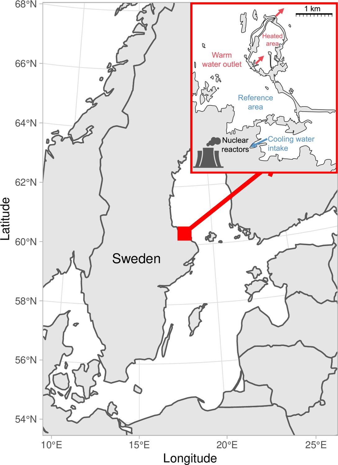
Map of the area with the unique whole-ecosystem warming experiment from which perch in this study was sampled.

Inset shows the 1 km² enclosed coastal bay that has been artificially heated for 23 years, the adjacent reference area with natural temperatures, and locations of the cooling water intake, and where the heated water outlet from nuclear power plants enters the heated coastal basin. The arrows indicate the direction of water flow.

Figure 2 with 10 supplements

Download asset Open asset

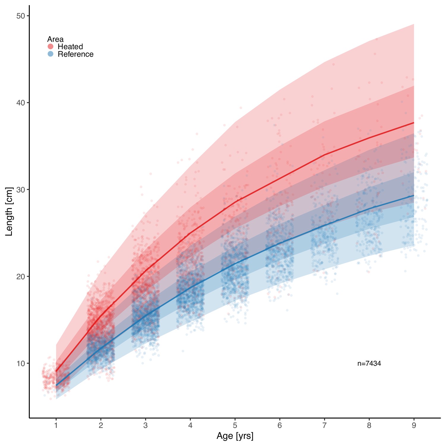
Fish grow faster and reach larger sizes in the heated enclosed bay (red) compared to the reference area (blue).

Points depict individual-level length-at-age and lines show the median of the posterior draws of the global posterior predictive distribution (without group-level effects), both exponentiated, from the von Bertalanffy growth model with area-specific coefficients. The shaded areas correspond to 50% and 90% credible intervals.

Figure 2—figure supplement 1

Download asset Open asset

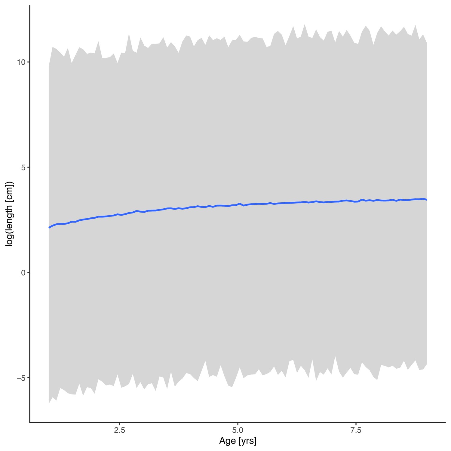
Prior predictive distribution for the von Bertalanffy growth equation (posterior draws from the prior only, ignoring the likelihood).

The solid line is the median and the shaded area is the 95% credible interval.

Figure 2—figure supplement 2

Download asset Open asset

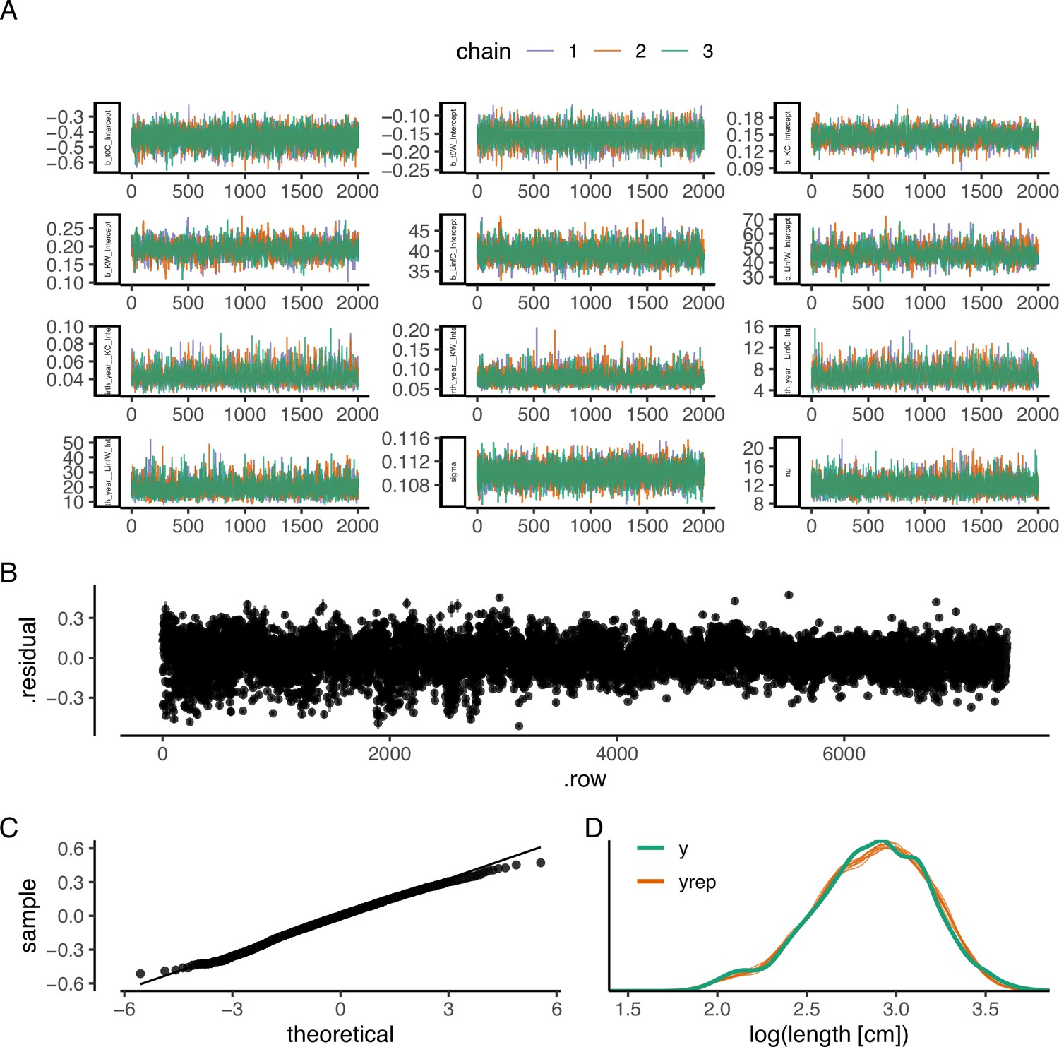
The best model of the von Bertalanffy growth equation: (A) trace plot to illustrate chain convergence for key (population-level) parameters, (B) residuals, (C) QQ-plot, and (D) posterior predictive check.

Figure 2—figure supplement 3

Download asset Open asset

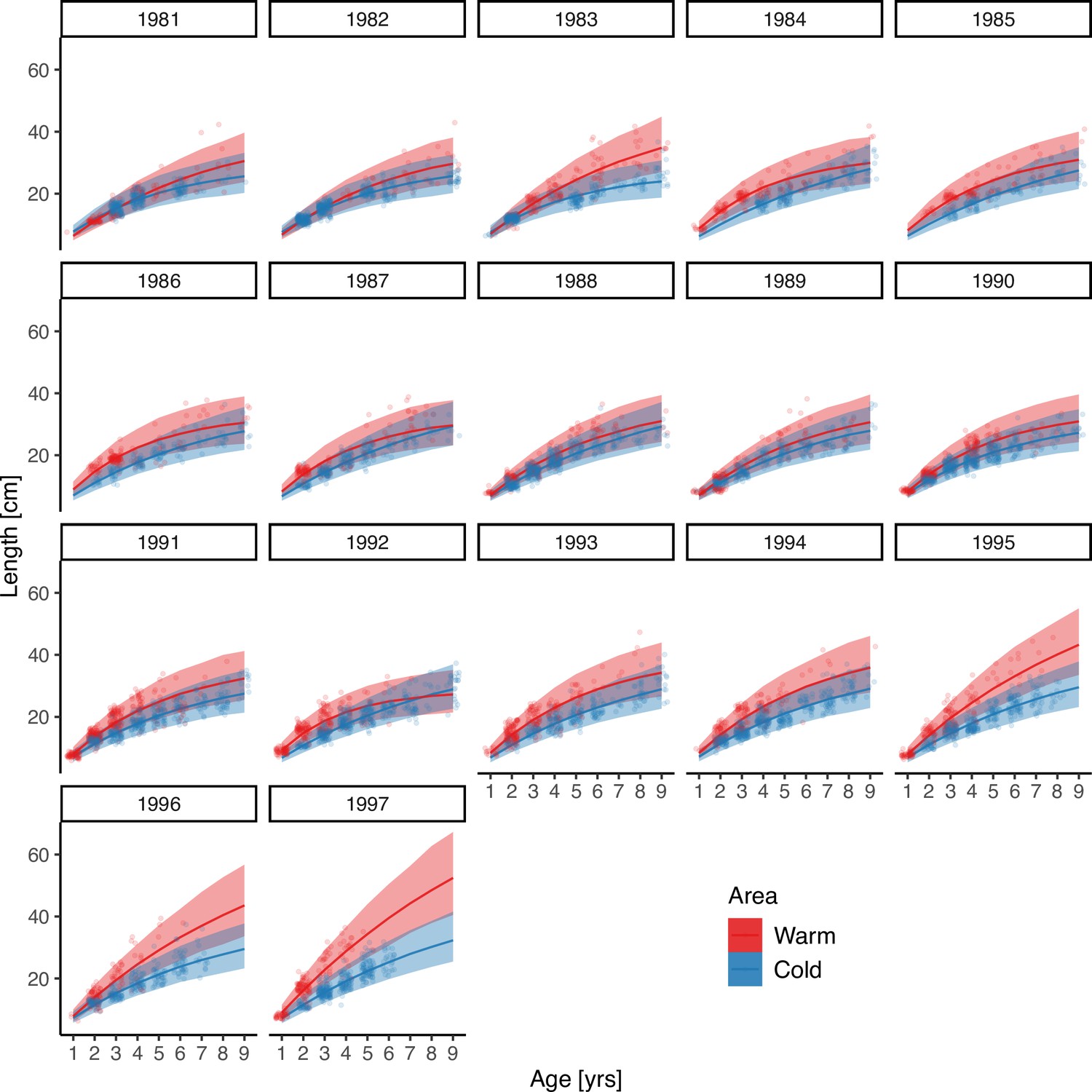
Cohort-specific predictions from the best von Bertalanffy model (i.e. with cohort-specific $L_{\infty}$ and $K$ ).

Points correspond to data; solid lines correspond to the median of the posterior prediction from the model and the shaded area corresponds to the 95% credible interval.

Figure 2—figure supplement 4

Download asset Open asset

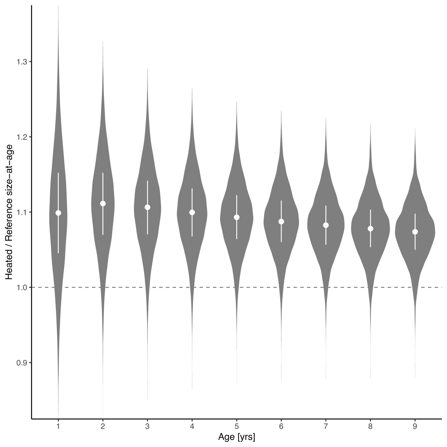
The average length-at-age is larger for fish of all ages in the heated enclosed bay compared to the reference area, and the relative difference declines very slightly with age.

Violin plots depict size-at-age in the heated relative to the reference area, based on draws from an expectation of the posterior predictive distribution (without random effects). The points and vertical lines depict the median and the interquartile range.

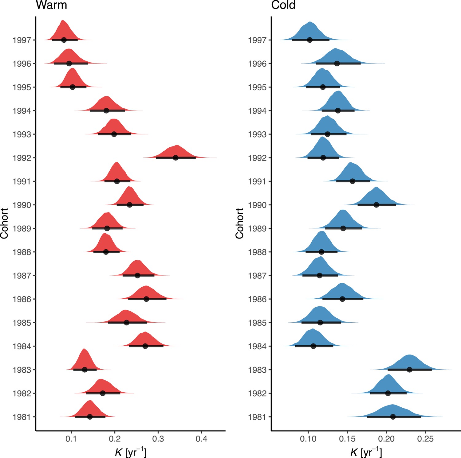
Figure 2—figure supplement 5

Download asset Open asset

Posterior distributions of the cohort-varying $L_{\infty}$ parameter in the best von Bertalanffy growth model.

Points correspond to the median and the horizontal lines correspond to the 95% credible interval. Note that the distributions of $L_{\infty}$ in the warm areas extend beyond the x-axis for cohorts 1995–1997 (also evident in Figure 3). The range of the x-axis was set to be wide enough to include the posterior medians of the larger estimates but narrow enough to allow for comparison between the other cohorts and areas.

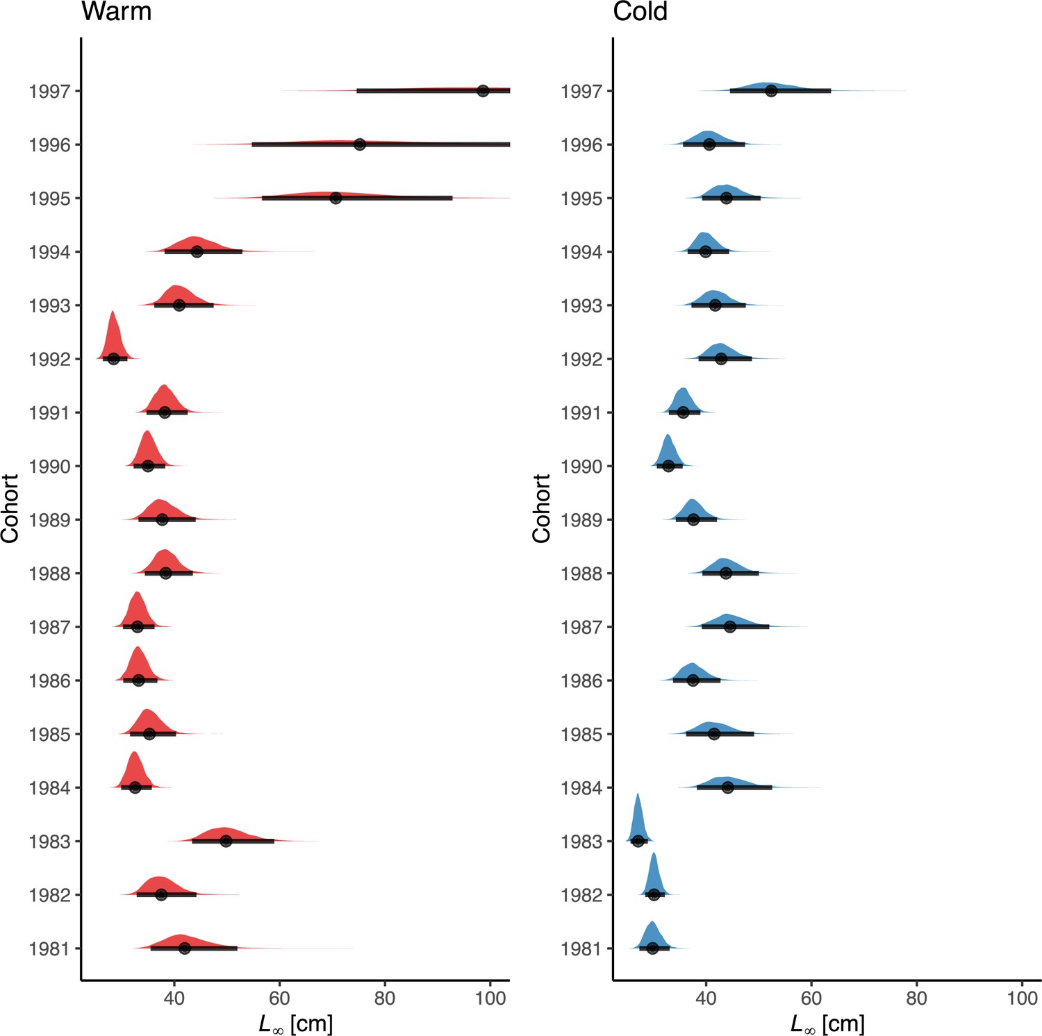
Figure 2—figure supplement 6

Download asset Open asset

Posterior distributions of the cohort-varying $K$ parameter in the von Bertalanffy model.

Points correspond to the median and the horizontal lines correspond to the 95% credible interval.

Figure 2—figure supplement 7

Download asset Open asset

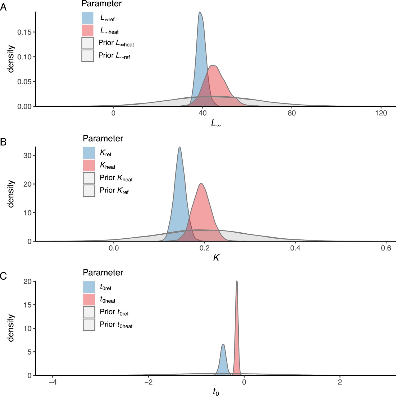
Prior vs posterior distributions for parameters $L_{\infty}$ (A), $K$ (B) and $t_{0}$ (C) in the best model of the von Bertalanffy growth equation.

Figure 2—figure supplement 8

Download asset Open asset

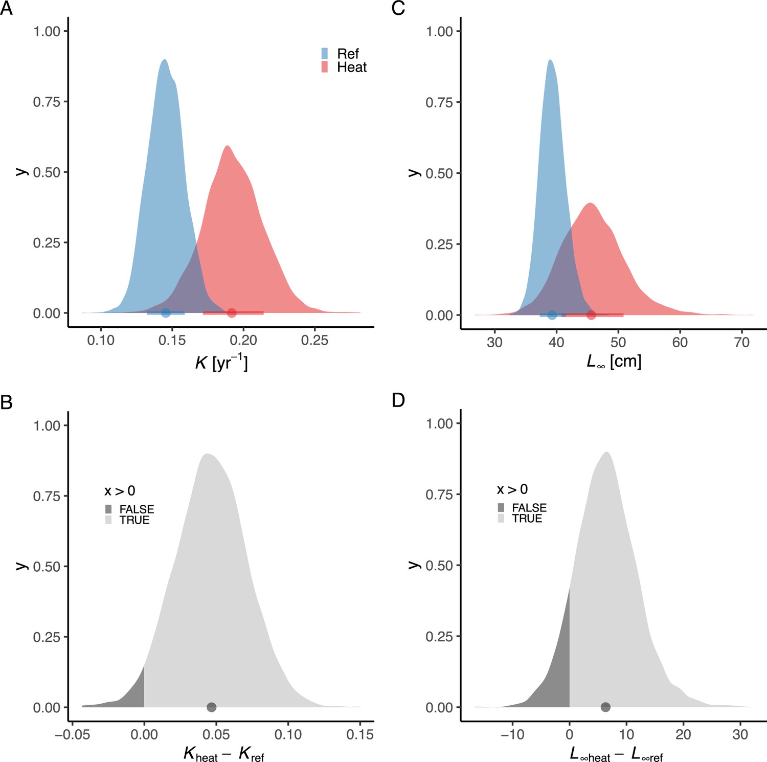
Posterior distributions of $K$ (A) and $L_{\infty}$ (B) for both areas and the distribution of their difference (**C, D**).

Panel (A) depicts the posterior distributions for the Brody growth coefficient (parameters $K_{h e a t}$ (red) and $K_{r e f}$ (blue)) and (B) the distribution of their difference. Panel (C) depicts the posterior distributions for asymptotic length (parameters $L_{\infty h e a t}$ and $L_{\infty r e f}$ ), and (D) the distribution of their difference (3%). The fill color depicts the area below 0 (3% and 11% for $K$ and $L_{\infty}$ , respectively).

Figure 2—figure supplement 9

Download asset Open asset

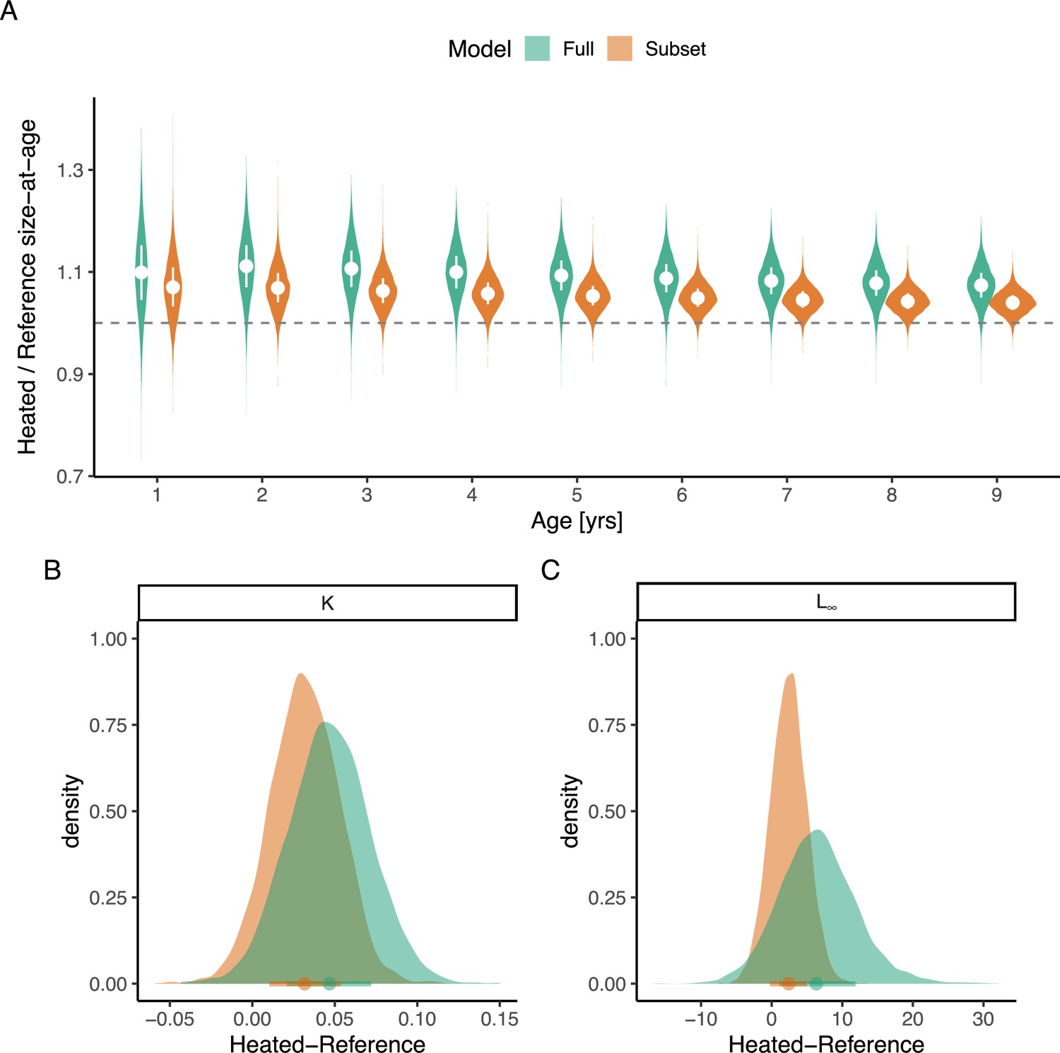
Analysis of sensitivity of including the most recent cohorts, with a smaller age range and, therefore, less certain estimates of $L_{\infty}$ .

Panel (A) depicts the predicted size-at-age from the full model (green) and the same model fitted without cohorts 1995–1997. The violin plots depict size-at-age in the heated relative to the reference area, based on draws from an expectation of the posterior predictive distribution (without random effects). The points and vertical lines depict the median and the interquartile range. Panels (B) and (C) depict the posterior distribution of differences in $K$ and $L_{\infty}$ , respectively, where color again indicates full or subset models.

Figure 2—figure supplement 10

Download asset Open asset

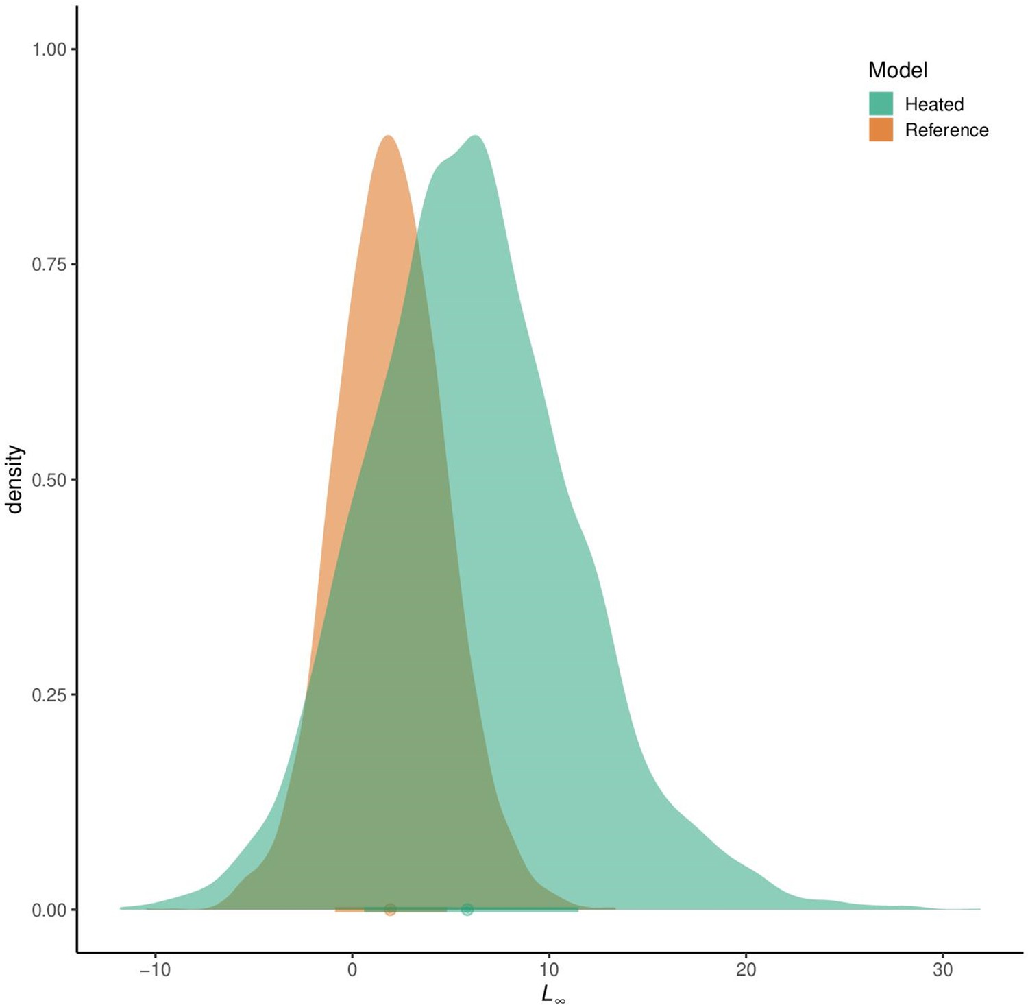
Analysis of sensitivity of including the most recent cohorts, with a smaller age range and, therefore, less certain estimates of $L_{\infty}$ .

The distributions depict the differences between the full and the subset models' posterior distributions for $L_{\infty}$ , with colors corresponding to the estimate for the heated and reference area.

Figure 3 with 3 supplements

Download asset Open asset

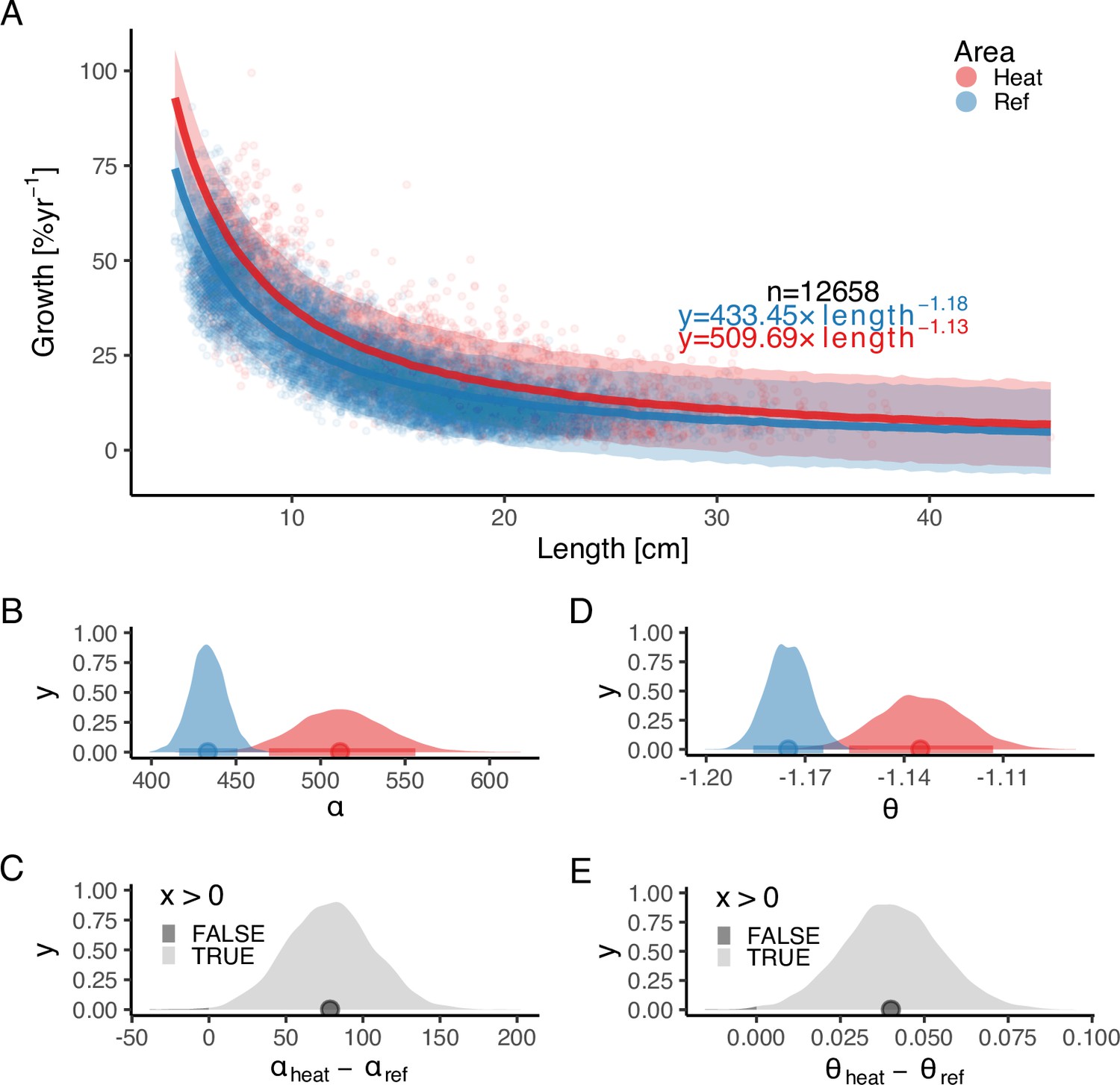
The faster growth rates in the heated area (red) compared to the reference (blue) are maintained as fish grow in size.

The points illustrate specific growth rate estimated from back-calculated length-at-age (within individuals) as a function of length, expressed as the geometric mean of the length at the start and end of the time interval. Lines show the median of the posterior draws of the global posterior predictive distribution (without group-level effects) from the allometric growth model with area-specific coefficients. The shaded areas correspond to the 90% credible interval. The equation uses mean parameter estimates. Panel (B) shows the posterior distributions for initial growth ( $α_{h e a t}$ (red) and $α_{r e f}$ (blue)), and (C) the distribution of their difference. Panel (D) shows the posterior distributions for the allometric exponent ( $θ_{h e a t}$ and $θ_{r e f}$ ), and (E) the distribution of their difference. The fill color depicts the area below 0 (0.3% and 0.2% for $α$ and $θ$ , respectively).

Figure 3—figure supplement 1

Download asset Open asset

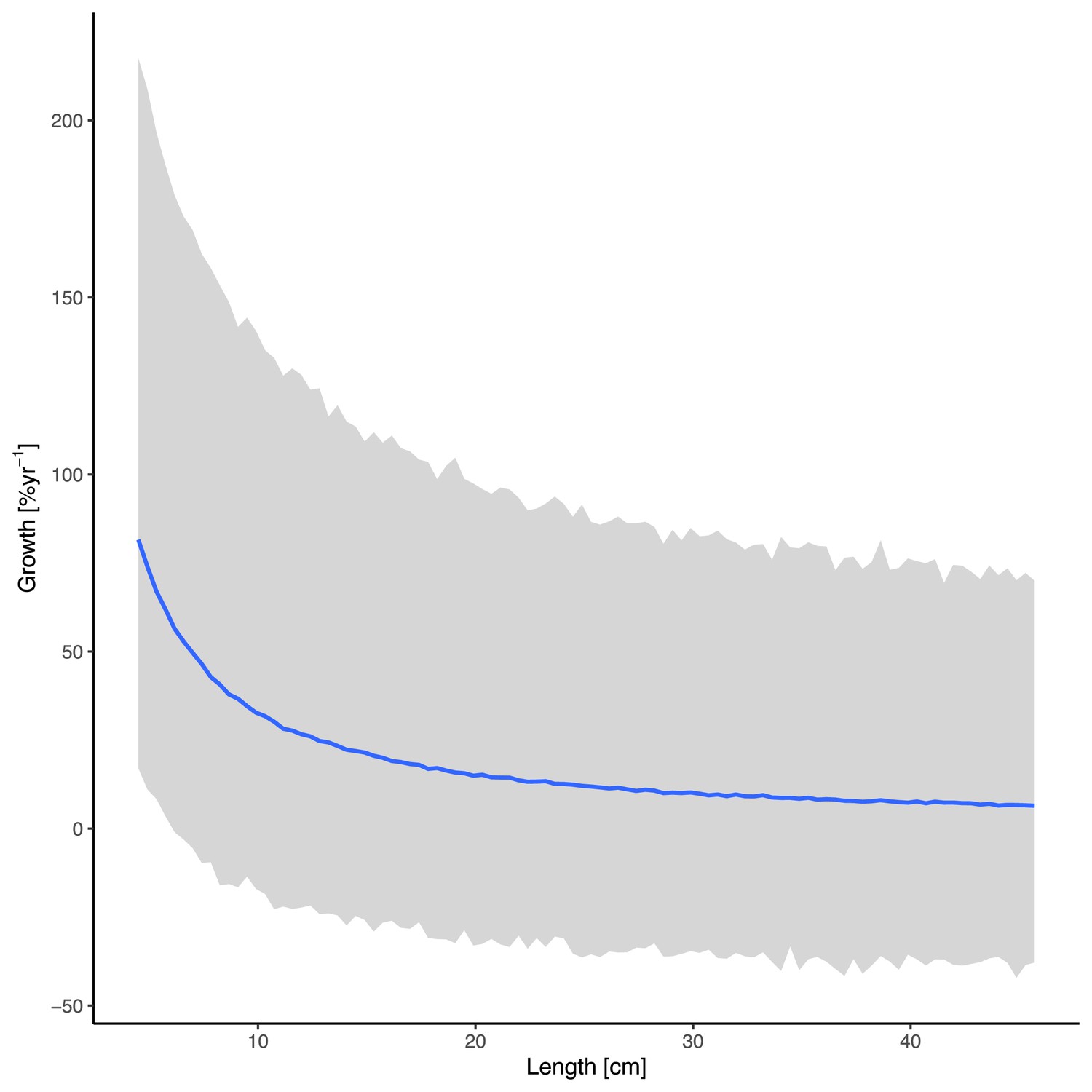
Prior predictive distribution for the allometric growth model (posterior draws from the prior only, ignoring the likelihood).

The solid line is the median and the shaded area is the 95% credible interval.

Figure 3—figure supplement 2

Download asset Open asset

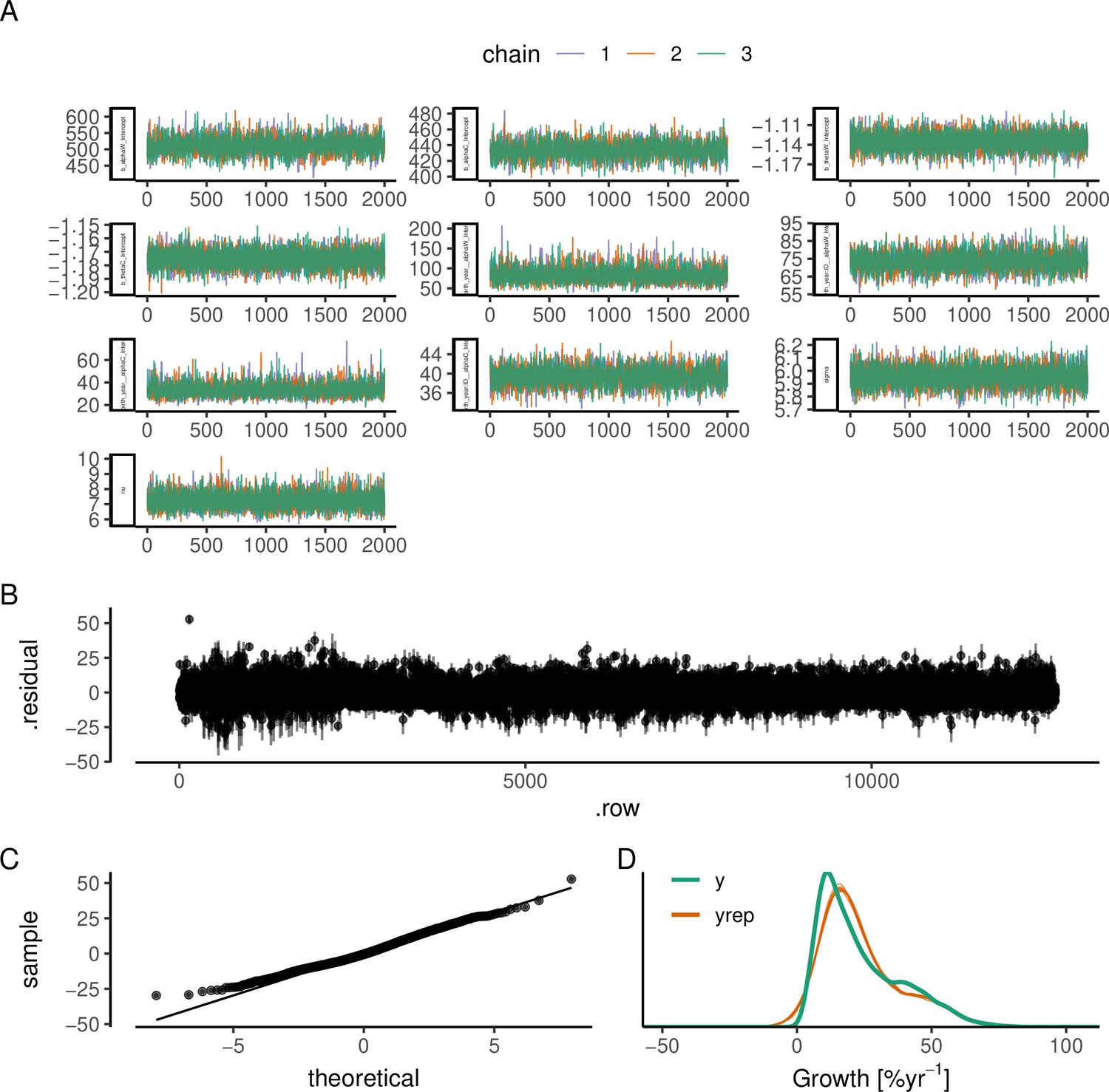
The best allometric growth model: (A) trace plot to illustrate chain convergence for key (population-level) parameters, (B) residuals, (C) QQ-plot, and (D) posterior predictive check.

Figure 3—figure supplement 3

Download asset Open asset

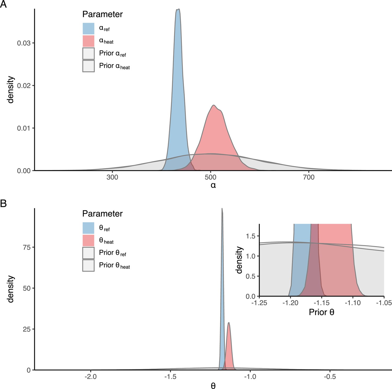
Prior vs posterior distributions for parameters $α$ (A) and $θ$ (B) in the best allometric growth model (inset in panel (B) is a zoomed-in version to better visualize the priors in the range of the posteriors).

Figure 4 with 2 supplements

Download asset Open asset

The instantaneous mortality rate ( $Z$ ) is higher in the heated area (red) than in the reference (blue).

Panel (A) shows $l o g (C P U E)$ as a function of $a g e$ , where the slope corresponds to $- Z$ . Lines show the median of the posterior draws of the global posterior predictive distribution (without group-level effects) and the shaded areas correspond to the 50% and 90% credible intervals. The equation shows mean parameter estimates. Panel (B) shows the posterior distributions for mortality rate ( $Z_{h e a t}$ and $Z_{r e f}$ ), and (C) the distribution of their difference, where the fill color depicts the area below 0 (0.07%).

Figure 4—figure supplement 1

Download asset Open asset

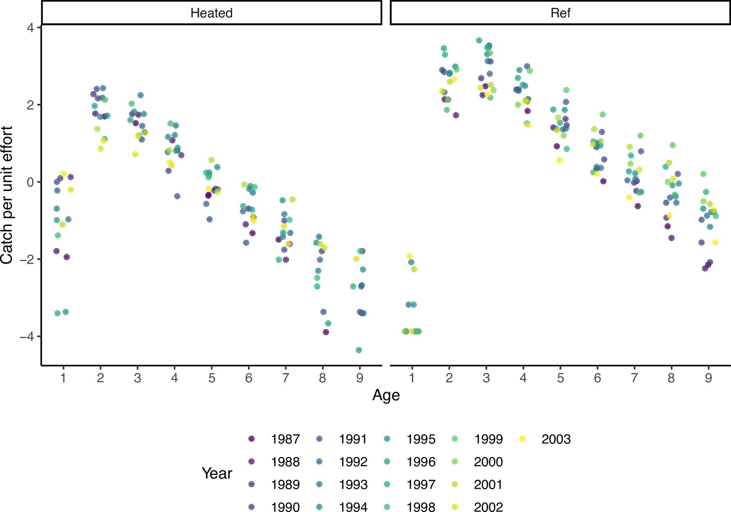
Catch per unit effort (CPUE) as a function of age, by area and year, for determining which ages are representatively caught by the fishing gear.

Since the CPUE starts to decline for fish older than 2 years, we selected only fish aged three or older for the catch curve regression analysis. Colors indicate catch year.

Figure 4—figure supplement 2

Download asset Open asset

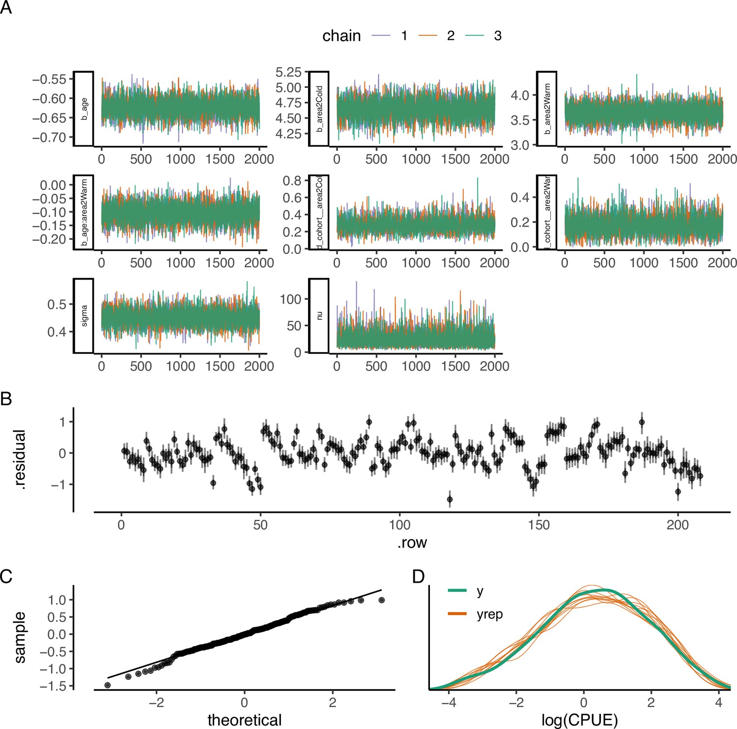
The best catch curve model: (A) trace plot to illustrate chain convergence for key (population-level) parameters, (B) residuals, (C) QQ-plot, and (D) posterior predictive check.

Figure 5

Download asset Open asset

The heated area (red) has a larger proportion of large fish than the reference area (blue), illustrated both in terms of histograms of proportions at size (A) and the biomass size-spectrum (**B, C**), but the difference in the slope of the size spectra between the areas is not statistically clear (C).

Panel (A) illustrates histograms of length groups in the heated and reference area as proportions (for all years pooled). Panel (B) shows the estimate of the size-spectrum exponent, $γ$ , where vertical lines depict the 95% confidence interval. Panel (C) shows the size distribution and MLEbins fit (red and blue solid curves for the heated and reference area, respectively) with 95% confidence intervals indicated by dotted lines. The vertical span of rectangles illustrates the possible range of the number of individuals with body mass ≥ the body mass of individuals in that bin.

Figure 6 with 2 supplements

Download asset Open asset

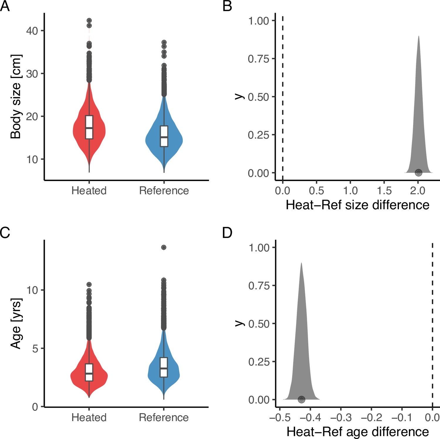
The average size is larger (**A, B**), but the average age (**C, D**) is younger in the heated area compared to the reference area.

The violin plots (**A, C**) are based on draws from the global posterior predictive distribution (without group-level effects) for mean size and age from the lognormal model, respectively, with the random year effect omitted, while the density plots (**B, D**) depict the difference between areas based on draws from the expected value of the posterior predictive distribution. Hence, the latter has a smaller variation and the difference in means is more pronounced. The average size is 2 cm larger in the heated area, and the average age is 0.4 years younger (**B, D**).

Figure 6—figure supplement 1

Download asset Open asset

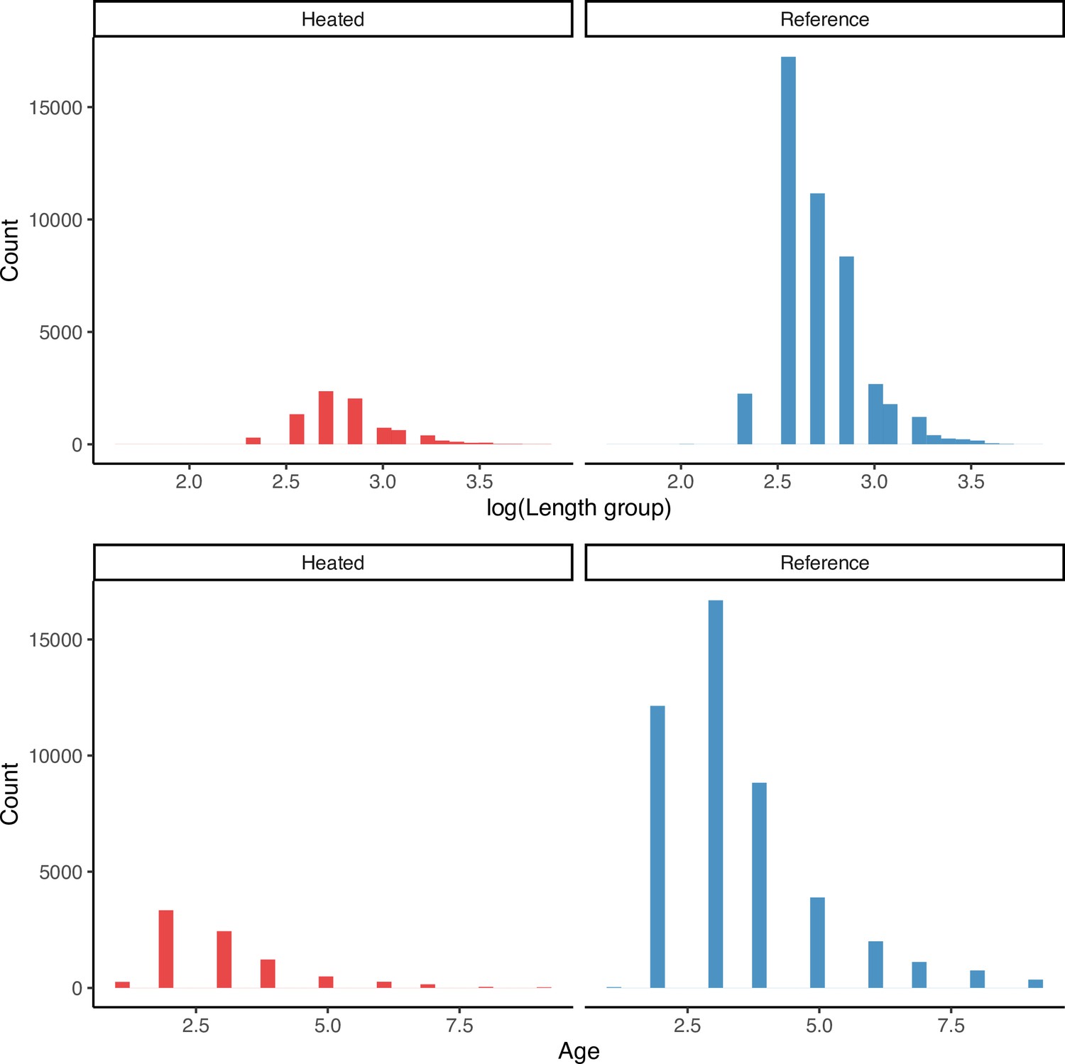
Size (top) and age (bottom) distribution of catches, all years pooled, as used in the lognormal model estimate the mean size and catch.

Heated area is shown in the left column (in red) and the reference area in the right (blue).

Figure 6—figure supplement 2

Download asset Open asset

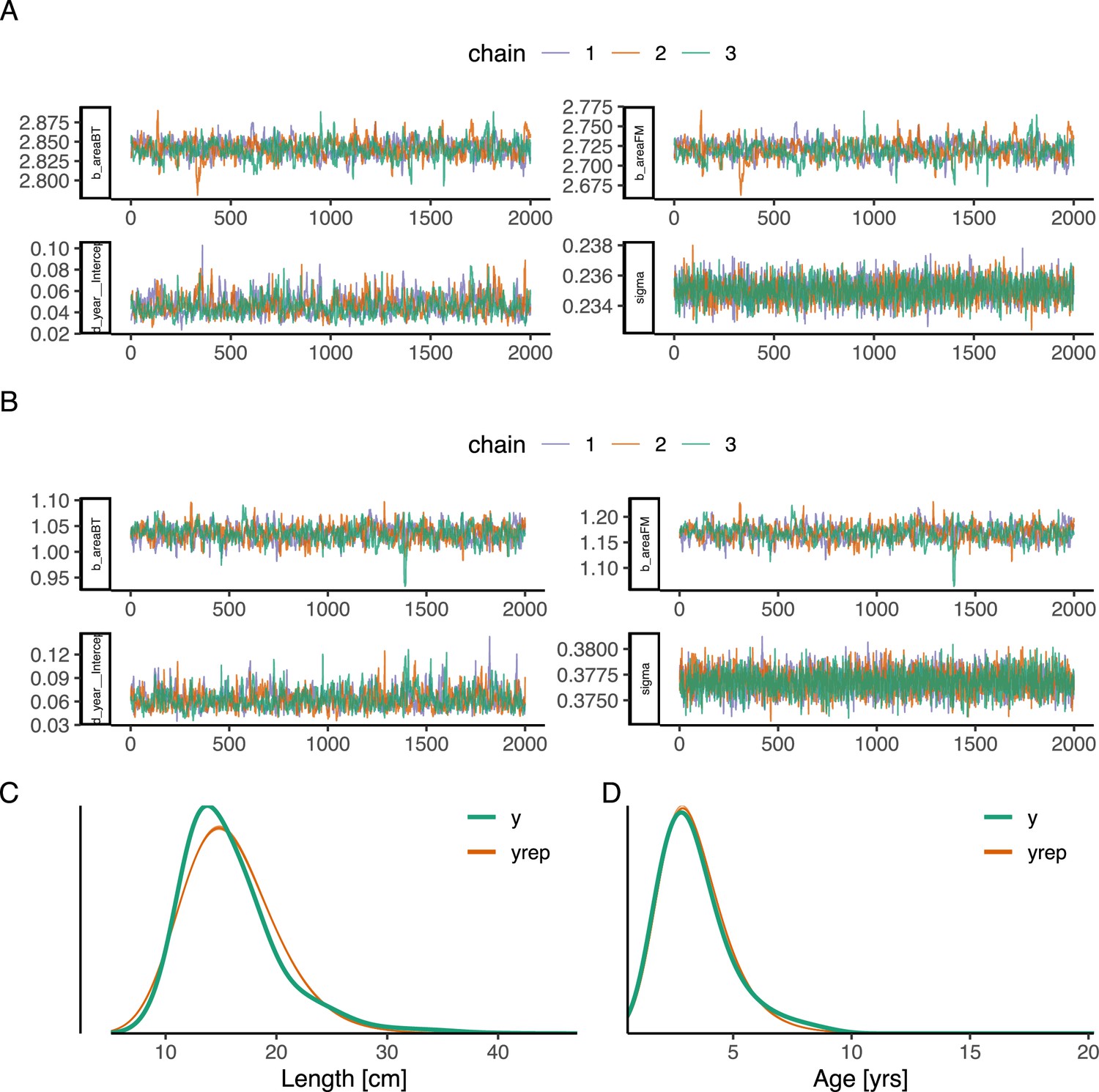
Lognormal length and age models model diagnostics and fit.

(**A–B**) trace plot to illustrate chain convergence for key (population-level) parameters in the lognormal length and age models (respectively), (**C–D**) posterior predictive checks for the length and the age model, respectively.

Additional files

Supplementary file 1 Expected log pointwise density (elpd) for different growth models. (a) Comparison of von Bertalanffy growth models with different combinations of shared and area-specific parameters (ordered by the difference in expected log pointwise density (elpd) from the best model). Note that in all models, ${L_{\infty}}_{j}$ and $K_{j}$ vary among cohorts. (b) Comparison of allometric growth models with common or unique $θ$ -parameter (exponent in the allometric growth model), ordered by the difference in expected log pointwise density (elpd) from the best model.: https://cdn.elifesciences.org/articles/82996/elife-82996-supp1-v1.docx
Download elife-82996-supp1-v1.docx
MDAR checklist: https://cdn.elifesciences.org/articles/82996/elife-82996-mdarchecklist1-v1.docx
Download elife-82996-mdarchecklist1-v1.docx

Download links

A two-part list of links to download the article, or parts of the article, in various formats.

Downloads (link to download the article as PDF)

Open citations (links to open the citations from this article in various online reference manager services)

Mendeley

Cite this article (links to download the citations from this article in formats compatible with various reference manager tools)

Max Lindmark
Malin Karlsson
Anna Gårdmark

(2023)

Larger but younger fish when growth outpaces mortality in heated ecosystem

eLife 12:e82996.

https://doi.org/10.7554/eLife.82996

Figures

Map of the area with the unique whole-ecosystem warming experiment from which perch in this study was sampled.

Fish grow faster and reach larger sizes in the heated enclosed bay (red) compared to the reference area (blue).

Prior predictive distribution for the von Bertalanffy growth equation (posterior draws from the prior only, ignoring the likelihood).

The best model of the von Bertalanffy growth equation: (A) trace plot to illustrate chain convergence for key (population-level) parameters, (B) residuals, (C) QQ-plot, and (D) posterior predictive check.

Cohort-specific predictions from the best von Bertalanffy model (i.e. with cohort-specific $L_{\infty}$ and $K$ ).

The average length-at-age is larger for fish of all ages in the heated enclosed bay compared to the reference area, and the relative difference declines very slightly with age.

Posterior distributions of the cohort-varying $L_{\infty}$ parameter in the best von Bertalanffy growth model.

Posterior distributions of the cohort-varying $K$ parameter in the von Bertalanffy model.

Prior vs posterior distributions for parameters $L_{\infty}$ (A), $K$ (B) and $t_{0}$ (C) in the best model of the von Bertalanffy growth equation.

Posterior distributions of $K$ (A) and $L_{\infty}$ (B) for both areas and the distribution of their difference (C, D).

Analysis of sensitivity of including the most recent cohorts, with a smaller age range and, therefore, less certain estimates of $L_{\infty}$ .

Analysis of sensitivity of including the most recent cohorts, with a smaller age range and, therefore, less certain estimates of $L_{\infty}$ .

The faster growth rates in the heated area (red) compared to the reference (blue) are maintained as fish grow in size.

Prior predictive distribution for the allometric growth model (posterior draws from the prior only, ignoring the likelihood).

The best allometric growth model: (A) trace plot to illustrate chain convergence for key (population-level) parameters, (B) residuals, (C) QQ-plot, and (D) posterior predictive check.

Prior vs posterior distributions for parameters $α$ (A) and $θ$ (B) in the best allometric growth model (inset in panel (B) is a zoomed-in version to better visualize the priors in the range of the posteriors).

The instantaneous mortality rate ( $Z$ ) is higher in the heated area (red) than in the reference (blue).

Catch per unit effort (CPUE) as a function of age, by area and year, for determining which ages are representatively caught by the fishing gear.

The best catch curve model: (A) trace plot to illustrate chain convergence for key (population-level) parameters, (B) residuals, (C) QQ-plot, and (D) posterior predictive check.

The heated area (red) has a larger proportion of large fish than the reference area (blue), illustrated both in terms of histograms of proportions at size (A) and the biomass size-spectrum (B, C), but the difference in the slope of the size spectra between the areas is not statistically clear (C).

The average size is larger (A, B), but the average age (C, D) is younger in the heated area compared to the reference area.

Size (top) and age (bottom) distribution of catches, all years pooled, as used in the lognormal model estimate the mean size and catch.

Lognormal length and age models model diagnostics and fit.

Additional files

Supplementary file 1

MDAR checklist

Download links

Downloads (link to download the article as PDF)

Open citations (links to open the citations from this article in various online reference manager services)

Cite this article (links to download the citations from this article in formats compatible with various reference manager tools)

Be the first to read new articles from eLife

Share this article

Cite this article

Map of the area with the unique whole-ecosystem warming experiment from which perch in this study was sampled.

Fish grow faster and reach larger sizes in the heated enclosed bay (red) compared to the reference area (blue).

Prior predictive distribution for the von Bertalanffy growth equation (posterior draws from the prior only, ignoring the likelihood).

The best model of the von Bertalanffy growth equation: (A) trace plot to illustrate chain convergence for key (population-level) parameters, (B) residuals, (C) QQ-plot, and (D) posterior predictive check.

Cohort-specific predictions from the best von Bertalanffy model (i.e. with cohort-specific L∞ and K).

The average length-at-age is larger for fish of all ages in the heated enclosed bay compared to the reference area, and the relative difference declines very slightly with age.

Posterior distributions of the cohort-varying L∞ parameter in the best von Bertalanffy growth model.

Posterior distributions of the cohort-varying K parameter in the von Bertalanffy model.

Prior vs posterior distributions for parameters L∞ (A), K (B) and t0 (C) in the best model of the von Bertalanffy growth equation.

Posterior distributions of K (A) and L∞ (B) for both areas and the distribution of their difference (C, D).

Analysis of sensitivity of including the most recent cohorts, with a smaller age range and, therefore, less certain estimates of L∞.

Analysis of sensitivity of including the most recent cohorts, with a smaller age range and, therefore, less certain estimates of L∞.

The faster growth rates in the heated area (red) compared to the reference (blue) are maintained as fish grow in size.

Prior predictive distribution for the allometric growth model (posterior draws from the prior only, ignoring the likelihood).

The best allometric growth model: (A) trace plot to illustrate chain convergence for key (population-level) parameters, (B) residuals, (C) QQ-plot, and (D) posterior predictive check.

Prior vs posterior distributions for parameters α (A) and θ (B) in the best allometric growth model (inset in panel (B) is a zoomed-in version to better visualize the priors in the range of the posteriors).

The instantaneous mortality rate (Z) is higher in the heated area (red) than in the reference (blue).

Catch per unit effort (CPUE) as a function of age, by area and year, for determining which ages are representatively caught by the fishing gear.

The best catch curve model: (A) trace plot to illustrate chain convergence for key (population-level) parameters, (B) residuals, (C) QQ-plot, and (D) posterior predictive check.

The heated area (red) has a larger proportion of large fish than the reference area (blue), illustrated both in terms of histograms of proportions at size (A) and the biomass size-spectrum (B, C), but the difference in the slope of the size spectra between the areas is not statistically clear (C).

The average size is larger (A, B), but the average age (C, D) is younger in the heated area compared to the reference area.

Size (top) and age (bottom) distribution of catches, all years pooled, as used in the lognormal model estimate the mean size and catch.

Lognormal length and age models model diagnostics and fit.

Supplementary file 1

MDAR checklist

Downloads (link to download the article as PDF)

Open citations (links to open the citations from this article in various online reference manager services)

Cite this article (links to download the citations from this article in formats compatible with various reference manager tools)

Cohort-specific predictions from the best von Bertalanffy model (i.e. with cohort-specific $L_{\infty}$ and $K$ ).

Posterior distributions of the cohort-varying $L_{\infty}$ parameter in the best von Bertalanffy growth model.

Posterior distributions of the cohort-varying $K$ parameter in the von Bertalanffy model.

Prior vs posterior distributions for parameters $L_{\infty}$ (A), $K$ (B) and $t_{0}$ (C) in the best model of the von Bertalanffy growth equation.

Posterior distributions of $K$ (A) and $L_{\infty}$ (B) for both areas and the distribution of their difference (C, D).

Analysis of sensitivity of including the most recent cohorts, with a smaller age range and, therefore, less certain estimates of $L_{\infty}$ .

Analysis of sensitivity of including the most recent cohorts, with a smaller age range and, therefore, less certain estimates of $L_{\infty}$ .

Prior vs posterior distributions for parameters $α$ (A) and $θ$ (B) in the best allometric growth model (inset in panel (B) is a zoomed-in version to better visualize the priors in the range of the posteriors).

The instantaneous mortality rate ( $Z$ ) is higher in the heated area (red) than in the reference (blue).