Temporal integration is a robust feature of perceptual decisions
- Centre de Recerca Matemàtica, Spain
- Princeton Neuroscience Institute, Princeton University, United States
- Institut d’Investigacions Biomèdiques August Pi i Sunyer (IDIBAPS), United States
- Laboratory of Sensorimotor Research, National Eye Institute, National Institutes of Health, United States
- Fuster Laboratory for Cognitive Neuroscience, Departments of Psychiatry & Biobehavioral Sciences and Ophthalmology, UCLA, United States
Figures
Figure 1
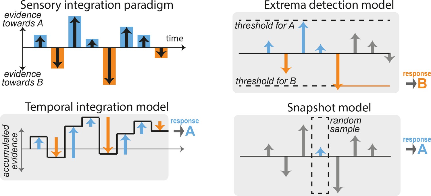
Integration and non-integration models for performing sensory discrimination tasks.
(A) Schematic of a typical fixed-duration perceptual task with discrete-sample stimuli (DSS). A stimulus is composed of a discrete sequence of n samples (here, n = 8). The subjects must report at the end of the sequence whether one specific quality of the stimulus was ‘overall’ leaning more toward one of two possible categories A or B. Evidence in favor of category A or B varies across samples (blue and orange bars). (B) Temporal integration model. The relative evidence in favor of each category is accumulated sequentially as each new sample is presented (black line), resulting in temporal integration of the sequence evidence. The choice is determined by the end point of the accumulation process: here, the overall evidence in favor of category A is positive, so response A is selected. (C) Extrema-detection model. A decision is made whenever the instantaneous evidence for a given sample (blue and orange arrows) reaches a certain fixed threshold (dotted lines). The selected choice corresponds to the sign of the evidence of the sample that reaches the threshold (here, response B). Subsequent samples are ignored (gray bars). (D) Snapshot model. Here, only one sample is attended. Which sample is attended is determined in each trial by a stochastic policy. The response of the model simply depends on the evidence of the attended sample. Other samples are ignored (gray bars). Variants of the model include attending K > 1 sequential samples.
Figure 2 with 3 supplements
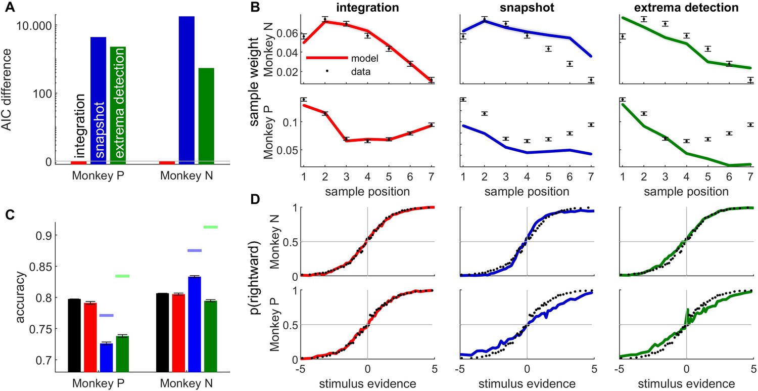
The integration model better described monkey behavior than non-integration models.
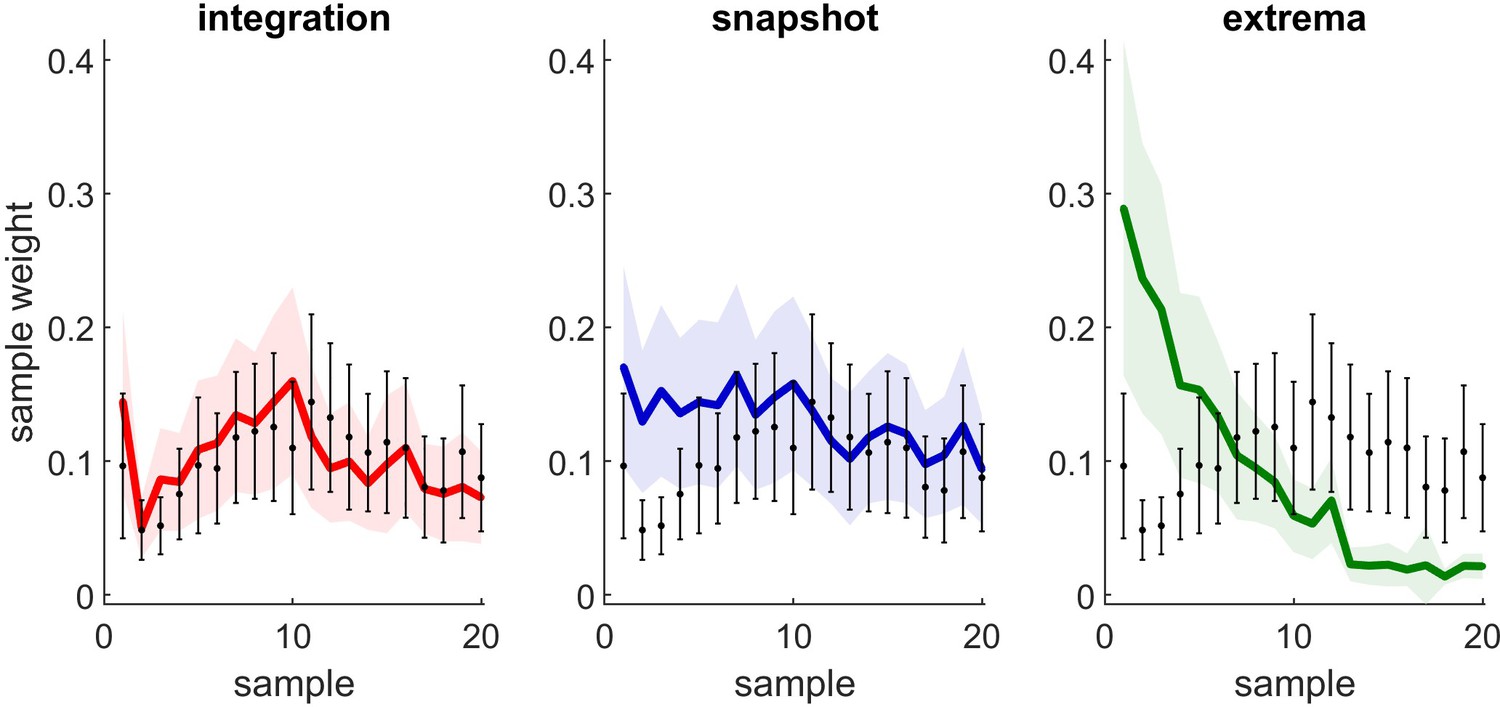
(A) Difference between Akaike information criterion (AIC) of models (temporal integration: red bar; snapshot model: blue; extrema-detection model: green) and temporal integration model for each monkey. Positive values indicate poorer fit to data. (B) Psychophysical kernels for behavioral data (black dots) vs. simulated data from temporal integration model (left panel, red curve), snapshot model (middle panel, blue curve), and extrema-detection model (right panel, green curve) for the two animals (monkey N: top panels; monkey P: bottom panels). Each data point represents the weight of the motion pulse at the corresponding position on the animal/model response. Error bars and shadowed areas represent the standard error of the weights for animal and simulated data, respectively. (C) Accuracy of animal responses (black bars) vs. simulated data from fitted models (color bars), for each monkey. Blue and green marks indicate the maximum performance for the snapshot and extrema-detection models, respectively. Error bars represent standard error of the mean. (D) Psychometric curves for animal (black dots) and simulated data (color lines) for monkey N, representing the proportion of rightward choices per quantile of weighted stimulus evidence.
Figure 2—figure supplement 1
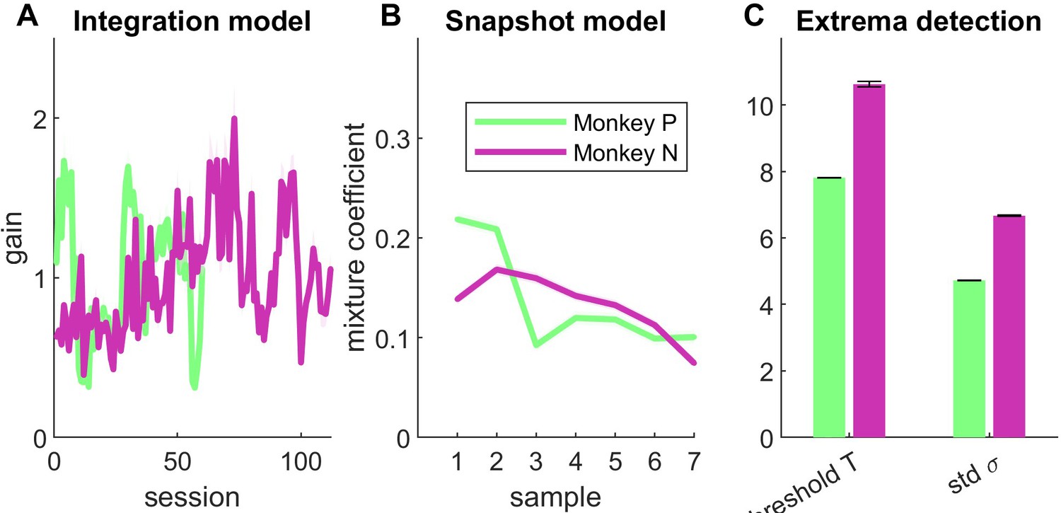
Parameter fits for integration and non-integration models.
(A) Modulation gain per session for the integration model, for each animal (green: monkey P; purple: monkey N). (B) Mixture coefficients of the snapshot model estimated for each monkey, representing the prior probability that each sample is attended on each trial. (C) Parameters T and of the extrema-detection model, estimated for each monkey. Error bars correspond to the confidence interval obtained using the Laplace approximation.
Figure 2—figure supplement 2
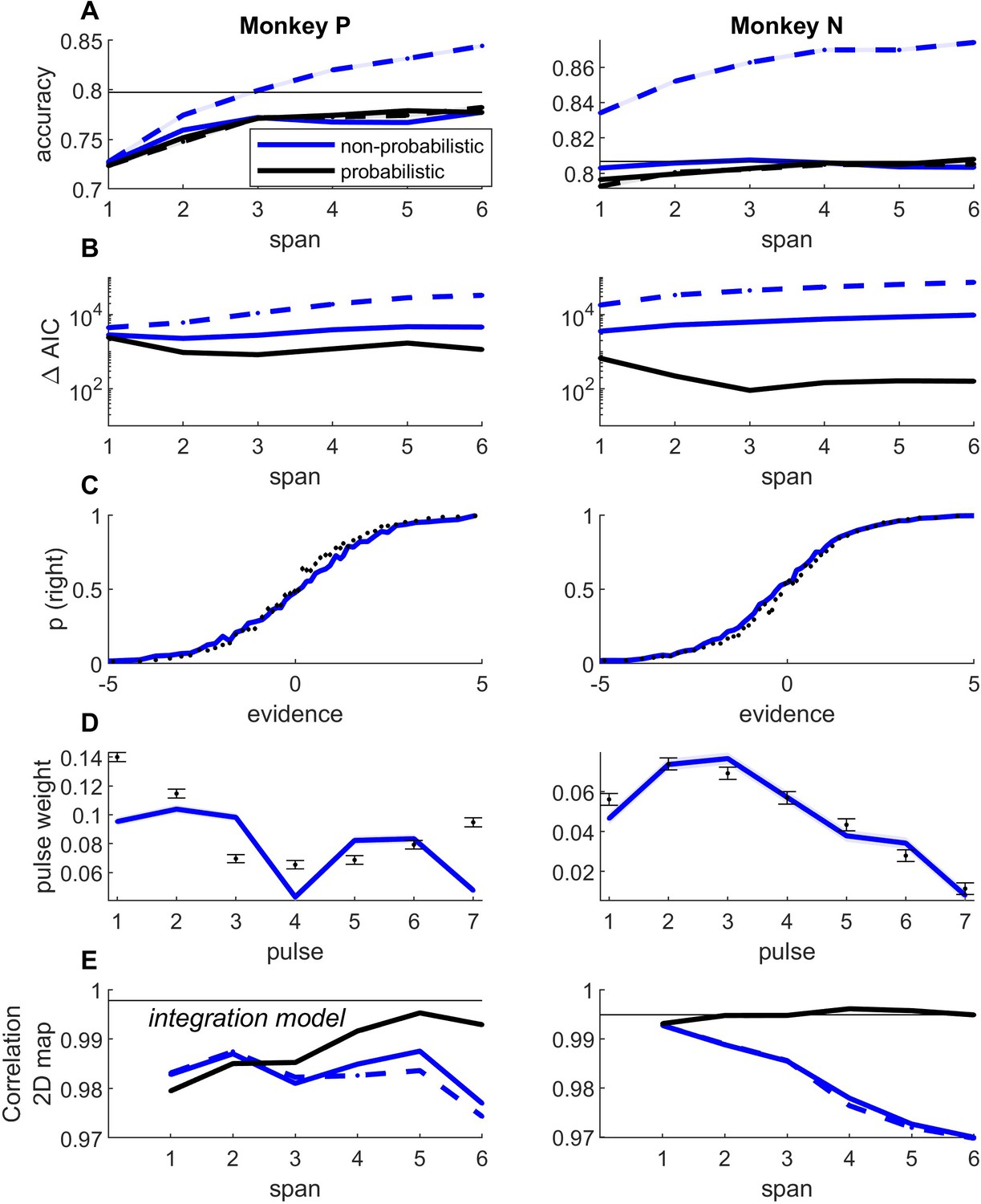
Model fits for variants of the snapshot model.
(A) Predicted accuracy for the snapshot model fitted to monkey data, as a function of memory span K, for fixed lapses (dashed lines, ) and lapses estimated from the data (full lines). Black curves represent the model with sensory noise (‘probabilistic’), blue curves represent the model without sensory noise (‘non-probabilistic’ or ‘deterministic’). Memory span K corresponds to the number of successive samples used to define the decision on each trial (see Methods). The horizontal bar corresponds to the average accuracy of the animal. (B) Akaike information criterion (AIC) difference between each of the four variants of the snapshot and the integration model. Legend as in A (full/dashed lines for fixed/free lapse parameters; black/blue curves for probabilistic/deterministic variants). Note that the probabilistic variant with either fixed or free lapses provide virtually indistinguishable values. Positive values indicate that the snapshot model provides a worse fit compared with the integration model. (C) Psychometric curve for the snapshot model with span K = 3 samples, sensory noise and free lapse parameters (best snapshot model variant according to AIC). (D) Psychophysical kernel for the same variant of the model. (E) Correlation between data and model integration maps for variants of the snapshot model.
Figure 2—figure supplement 3
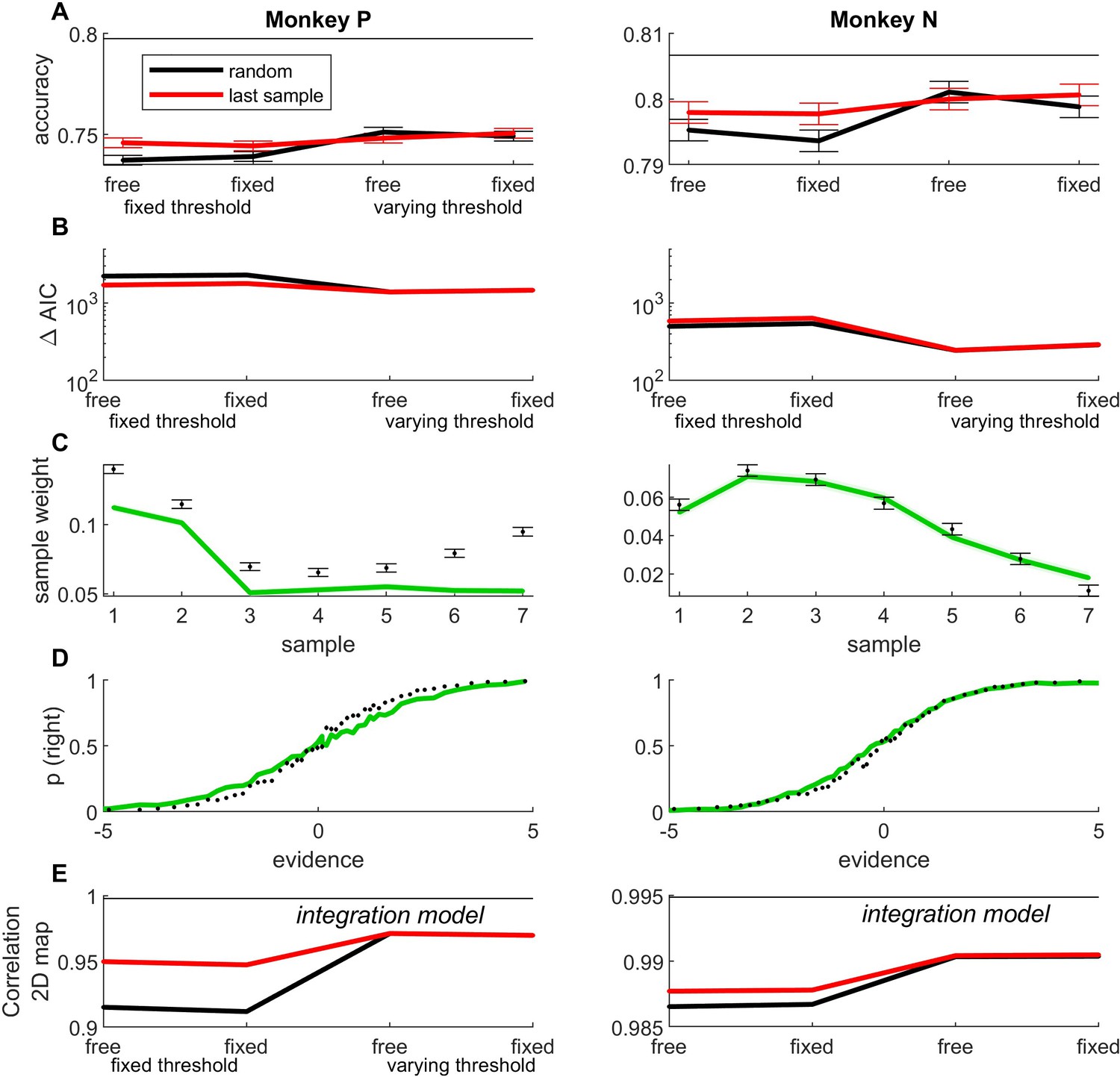
Model fits for variants of the extrema-detection model.
(A) Predicted accuracy for the extrema-detection model fitted to the monkey data, for random (black curves) and last sample (red curve) default rule, for fixed lapses () or lapse parameters estimated from the data, and for fixed- or varying-threshold parameter. The horizontal bar indicates animal accuracy. (B) Akaike information criterion (AIC) difference between variants of the extrema-detection model and the integration model. Legend as in A. Positive values indicate that the extrema-detection model provides a worse fit. Psychometric curve (C) and psychophysical kernel (D) for the model variant that provided the best match to behavior in terms of predicted accuracy and AIC: free lapse parameters and last sample rule. (E) Correlation between integration maps from animal and simulated data (see Figure 4) for variants of the extrema-detection model. The horizontal bar marks the correlation between experimental data and the integration model.
Figure 3 with 1 supplement
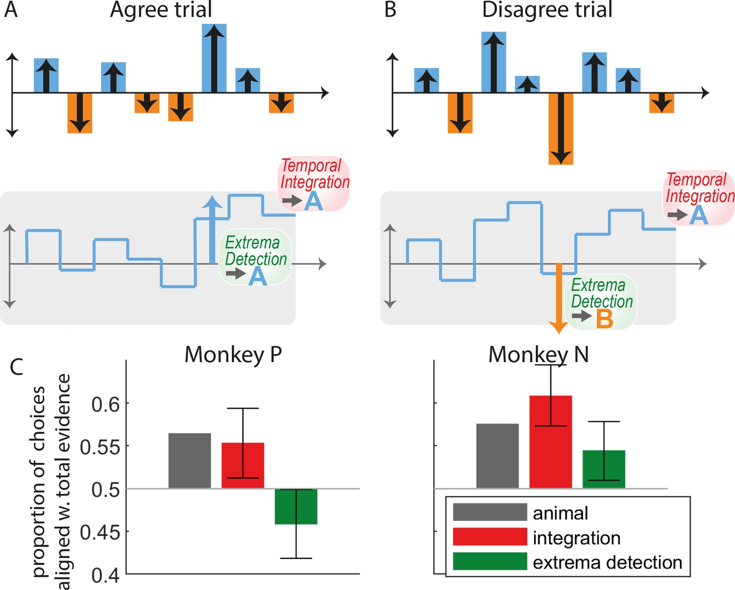
The pattern of animal choices is incompatible with extrema-value-based decisions.
(A) Example of an ‘agree trial’ where the total stimulus evidence (accumulated over samples) and the evidence from the largest evidence sample point toward the same response (here, response A). In this case, we expect that temporal integration and extrema-detection will produce similar responses (here, A). (B) Example of a ‘disagree trial’, where the total stimulus evidence and evidence from the largest evidence sample point toward opposite responses (here A for the former; B for the latter). In this case, we expect that integration and extrema-detection models will produce opposite responses. (C) Proportion of choices out of all disagree trials aligned with total evidence, for animal (gray bars), integration (red), and extrema-detection model (green). Error bars denote 95% confidence intervals based on parametric bootstrap (see Methods).
Figure 3—figure supplement 1
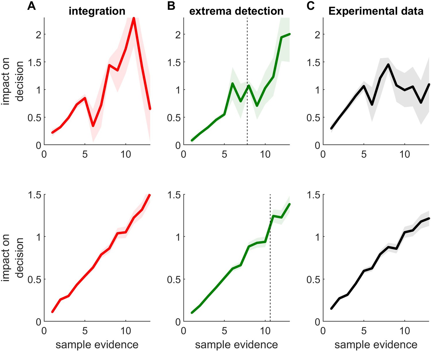
Subjective weights for animal data and simulated models.
Impact on decision of individual samples as a function of absolute sample evidence. Shaded area: standard error of the weight. Top row: monkey P; bottom row: monkey N. (A) Integration model. (B) Extrema-detection model. The vertical dotted line marks the value of the threshold T estimated from animal data. (C) Impact on decision of individual pulses, estimated from each monkey.
Figure 4 with 3 supplements
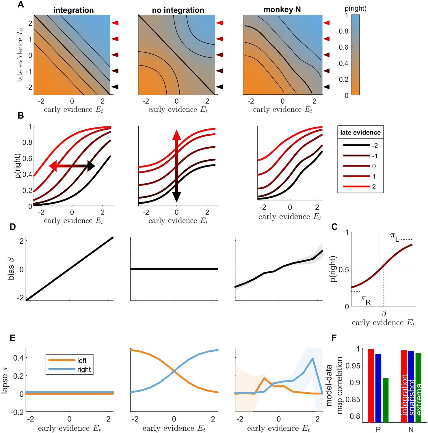
Integration of early and late evidence into animal responses is incompatible with the snapshot model.
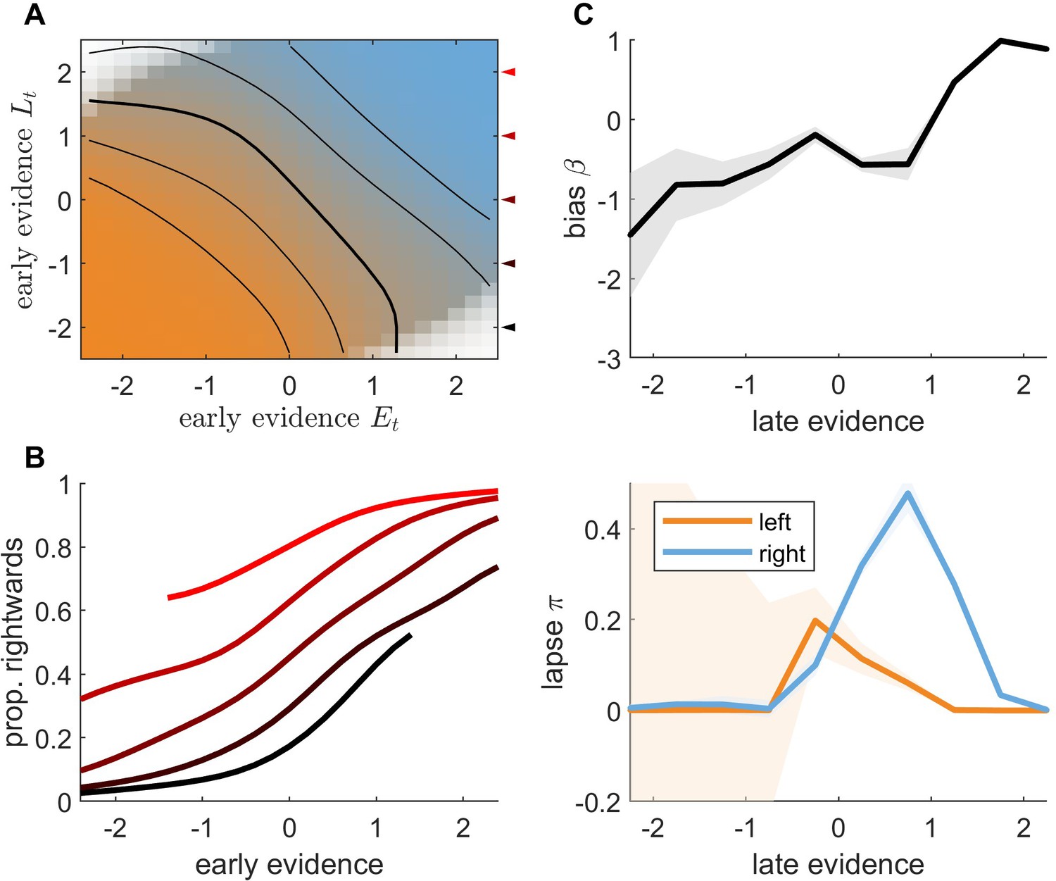
(A) Integration map representing the probability of rightward responses (orange: high probability; blue: low probability) as a function of early stimulus evidence and late stimulus evidence , illustrated for a toy integration model (where ; left panel) and a toy non-integration model (; middle panel), and computed for monkey N responses (right panel). Black lines represent the isolines for p(rightwards) = 0.15, 0.3, 0.5, 0.7, and 0.85. (B) Conditional psychometric curves representing the probability for rightward response as a function of early evidence , for different values of late evidence (see inset for values), for toy models and monkey N. The curves correspond to horizontal cuts in the integration maps at values marked by color triangles in panel A. (C) Illustration of the fits to conditional psychometric curves. The value of the bias , left lapse and right lapse are estimated from the conditional psychometric curves for each value of late evidence. (D) Lateral bias as a function of late evidence for toy models and monkey N. Shaded areas represent standard error of weights for animal data. (E) Lapse parameters (blue: left lapse; orange: right lapse) as a function of late evidence for toy models and monkey N. (F) Pearson correlation between integration maps for animal data and integration maps for simulated data, for each animal. Red: integration model; blue: snapshot model; green: extrema-detection model.
Figure 4—figure supplement 1
Integration of early and late evidence for monkey P.
(A) Integration map. Legend as in Figure 4A. (B) Conditional psychometric curves. Legend as in Figure 4B. (C) Bias and lapse parameters from conditional psychometric curves, as a function of late evidence. Legend as in Figure 4D, E.
Figure 4—figure supplement 2
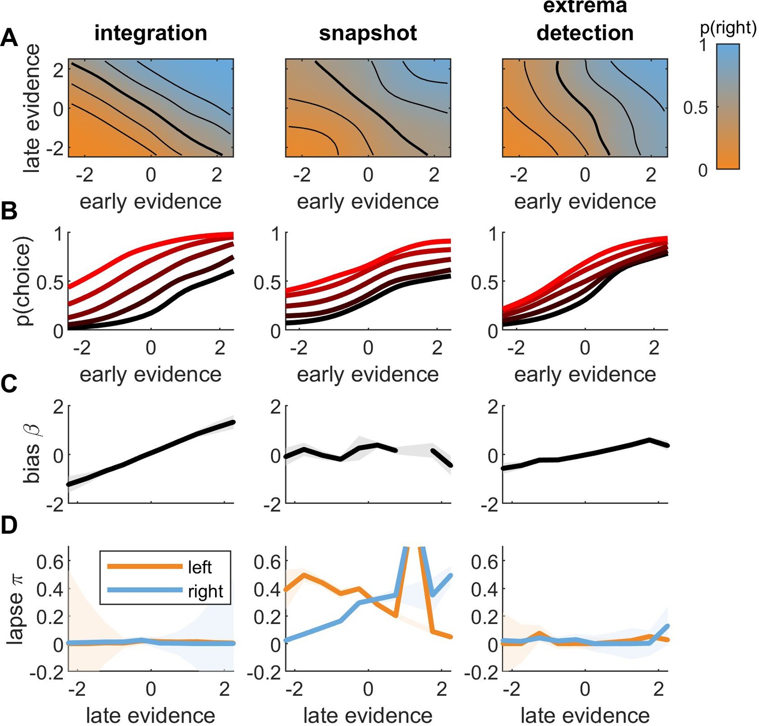
Integration between early and late evidence for simulated data from integration and non-integration models.
Data were simulated for each model from parameters estimated from monkey N. Left panels: integration model. Middle panels: snapshot models. Right panels: extrema-detection models. (A) Integration maps. (B) Conditional psychometric curves. (C) Lateral bias and (D) lapse parameters estimated from conditional psychometric curves, as a function late evidence. Legend as in Figure 4.
Figure 4—figure supplement 3
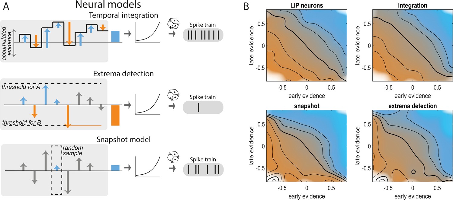
Individual Lateral Intra Parietal (LIP) neurons integrate sensory information over stimulus sequence.
(A) Neural models for temporal integration, extrema-detection, and snapshot model. (B) Integration map for LIP neurons, and simulated neurons following either integration, extrema-detection, or snapshot model. Color represents the average normalized spike count per bins of neuron-weighted early and late evidence (see Methods). Isolines represent values of 0.4, 0.6, 1, 1.4, and 1.8.
Figure 5 with 1 supplement
Behavioral data from orientation discrimination task in humans provide further evidence for temporal integration.
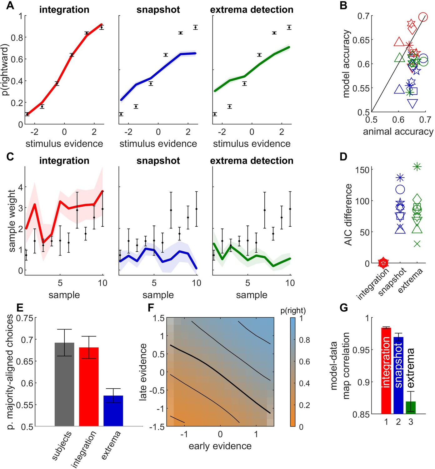
(A) Psychometric curves for human and simulated data, averaged across participants (n = 9). Legend as in Figure 2C. (B) Simulated model accuracy (y-axis) vs. participant accuracy (x-axis) for integration model (red), snapshot model (blue) and extrema-detection model (green). Each symbol corresponds to a participant. (C) Psychophysical kernel for human and simulated data, averaged across participants. Legend as in A. (D) Difference in Akaike information criterion (AIC) between each model and the integration model. Legend as in B. (E) Proportion of choices aligned with total stimulus evidence in disagree trials, for participant data (gray bars) and simulated models, averaged over participants. (F) Integration map for early and late stimulus evidence, computed as in Figure 4A, averaged across participants. (G) Correlation between integration map of participants and simulated data for integration, snapshot, and extrema-detection models, averaged across participants. Color code as in B. Error bars represent the standard error of the mean across participants in all panels.
Figure 5—figure supplement 1
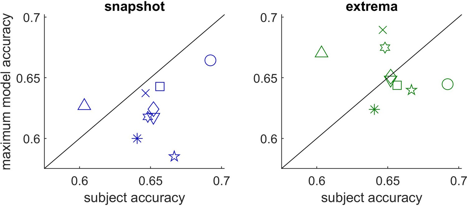
Maximum accuracy of the non-integration models vs. human subject accuracy in the orientation discrimination task.
Left panel: snapshot model (with span K = 1). Right panel: extrema-detection. Each symbol represents a subject.
Figure 6 with 1 supplement

Behavioral data from auditory discrimination task in five rats provide further evidence for temporal integration.
(A-G) Legend as in Figure 5. Rats were rewarded for correctly identifying the auditory sequence of larger intensity (number of samples: 10 or 20; stimulus duration: 500 or 1000 ms). Legend as in Figure 5. Psychophysical kernels are computed only for 10-sample stimuli (in 4 animals). See Figure 6—figure supplement 1 for psychophysical kernels with 20-sample stimuli.
Figure 6—figure supplement 1
Psychophysical kernels for animals and models in rats (n = 3) performing the discrete-sample stimulus (DSS) task with 20-sample stimuli.
Additional files
Download links
A two-part list of links to download the article, or parts of the article, in various formats.
Downloads (link to download the article as PDF)
Open citations (links to open the citations from this article in various online reference manager services)
Cite this article (links to download the citations from this article in formats compatible with various reference manager tools)
Temporal integration is a robust feature of perceptual decisions
eLife 12:e84045.
https://doi.org/10.7554/eLife.84045


