Using adversarial networks to extend brain computer interface decoding accuracy over time
- Department of Neuroscience, Northwestern University, United States
- Department of Biomedical Engineering, Northwestern University, United States
- Department of Physical Medicine and Rehabilitation, Northwestern University, United States
- Shirley Ryan AbilityLab, United States
Figures
Figure 1
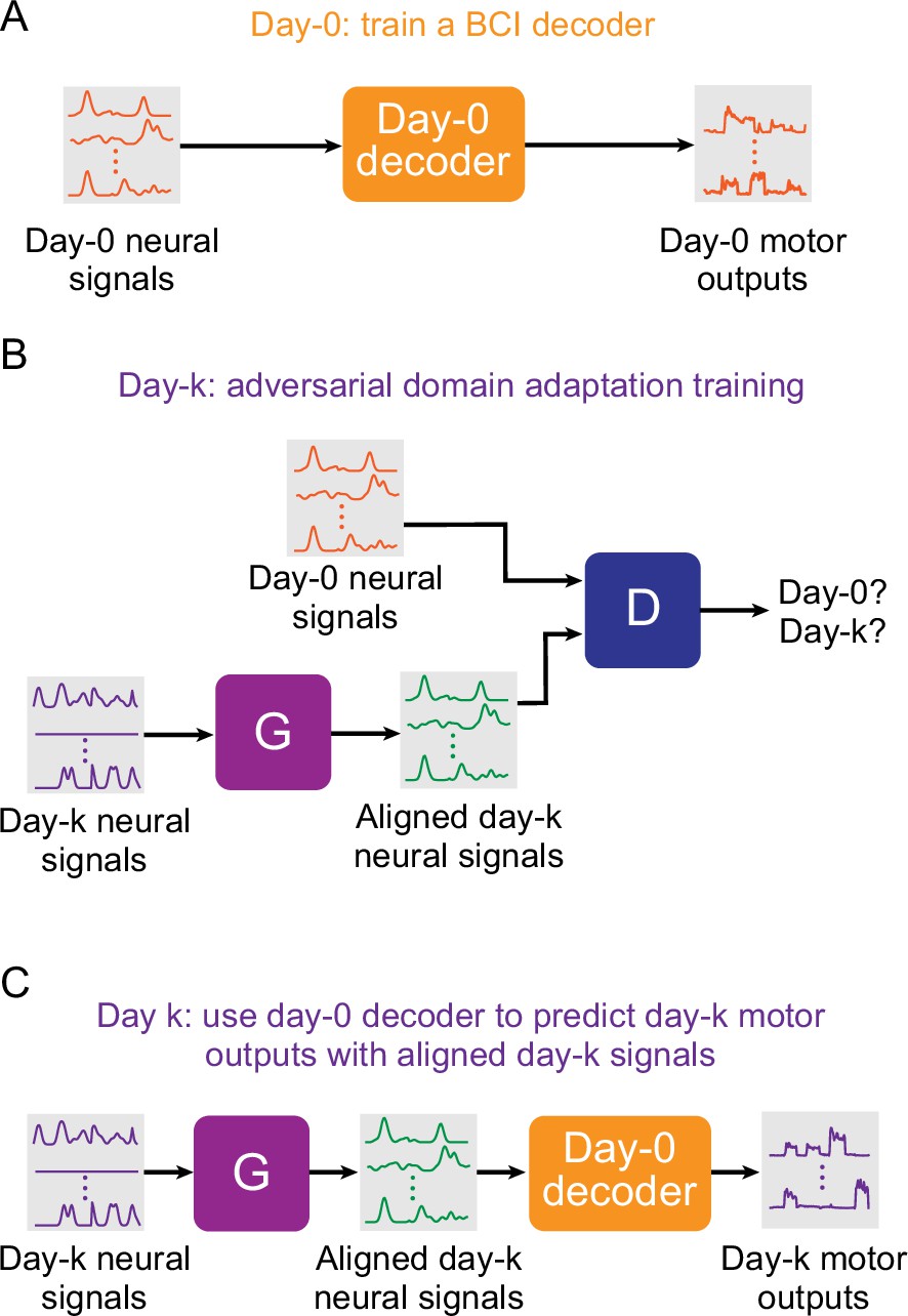
Setup for stabilizing an intracortical brain computer interface (iBCI) with adversarial domain adaptation.
(A) Initial iBCI decoder training on day-0. The decoder is computed to predict the motor outputs from neural signals, using either the full-dimensional neural recordings or the low-dimensional latent signals obtained through dimensionality reduction. This decoder will remain fixed over time after training. (B) A general framework for adversarial domain adaptation training on a subsequent day-k. The ‘Generator’ (G) is a feedforward neural network that takes day-k neural signals as the inputs and aims to transform them into a form similar to day-0 signals; we also refer to G as the ‘aligner’. The ‘Discriminator’ (D) is another feedforward neural network that takes both the outputs of G (aligned day-k neural signals) and day-0 neural signals as the inputs and aims to discriminate between them. (C) A trained aligner and the fixed day-0 decoder are used for iBCI decoding on day-k. The aligned signals generated by G are fed to the day-0 decoder to produce the predicted motor outputs.
Figure 2 with 4 supplements
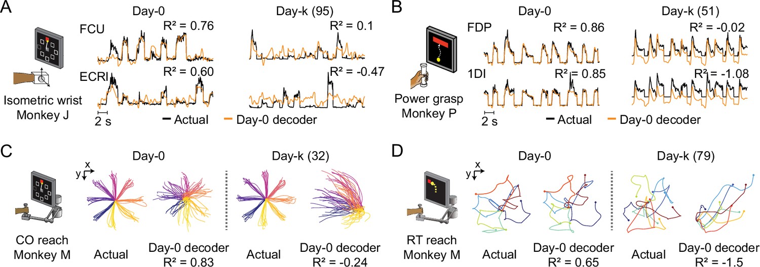
The performance of well-calibrated decoders declines over time.
(A) Actual EMGs (black) and predicted EMGs (orange) using the day-0 decoder for flexor carpi ulnaris (FCU) and extensor carpi radialis longus (ECRl) during the isometric wrist task. (B) Actual and predicted EMGs using the day-0 decoder for flexor digitorum profundus (FDP) and first dorsal interosseous (1DI) during the power grasp task. (C) Actual hand trajectories and predictions using the day-0 decoder during the center-out (CO) reach task. Colors represent different reaching directions. (D) Actual and predicted hand trajectories using the day-0 decoder during the random-target (RT) reach task. Colors represent different reaching directions.
-
Figure 2—source data 1
Table summarizing the datasets analyzed in this paper, including cortical implant site and date, number of recording sessions, number of days between recording start and end, recording days relative to time of array implantation, and motor outputs (EMG or hand velocities) recorded.
- https://cdn.elifesciences.org/articles/84296/elife-84296-fig2-data1-v2.docx
Figure 2—figure supplement 1
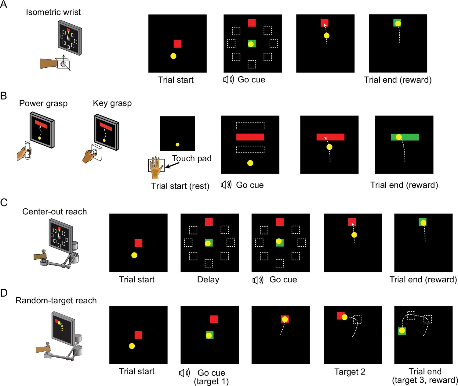
Behavior tasks.
(A) The structure of the isometric wrist task. Each trial started with the appearance of a center target requiring the monkeys to hold for a random time (0.2–1.0 s), after which one of eight possible outer targets selected in a block-randomized fashion appeared, accompanied with an auditory go cue. The monkey was allowed to move the cursor to the target within 2.0 s and hold for 0.8 s to receive a liquid reward. (B) The structure of the grasping tasks. At the beginning of each trial the monkey was required to keep the hand resting on a touch pad for a random time (0.5–1.0 s). A successful holding triggered the onset of one of three possible rectangular targets on the screen and an auditory go cue. The monkey was required to place the cursor into the target and hold for 0.6 s by increasing and maintaining the grasping force applied on the gadget. (C) The structure of the center-out (CO) reach task. At the beginning of each trial, the monkey needed to move the hand to the center of the workspace. One of eight possible outer targets equally spaced in a circle was presented to the monkey after a random waiting period. The monkey needed to keep holding for a variable delay period until receiving an auditory go cue. To receive a liquid reward, the monkey was required to reach the outer target within 1.0 s and hold within the target for 0.5 s. (D) The structure of the random-target (RT) reach task. At the beginning of each trial the monkey also needed to move the hand to the center of the workspace. Three targets were then presented to the monkey sequentially, and the monkey was required to move the cursor into each of them within 2.0 s after viewing each target. The positions of these targets were randomly selected, thus the cursor trajectory for each trial presented a ‘random-target’ manner.
Figure 2—figure supplement 2
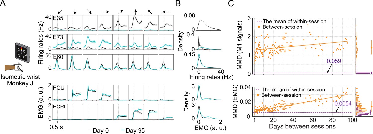
Unstable neural recordings underlying stable motor outputs.
Data from monkey J, who was trained to perform the isometric wrist task. (A) Peri-event time histograms (PETHs) for the multiunit activity from three cortical electrodes (E35, E73, E60) and the EMGs from two forearm muscles (flexor carpi ulnaris, FCU; extensor carpi radialis longus, ECRl) on day 0 and day 95. Each column corresponds to a target direction indicated by the arrows on the top. For each direction, 15 trials were averaged to get the mean values (solid lines) and the standard errors (shaded area). The dashed vertical line in each subplot indicates the timing of force onset. While the neural activity picked by the implanted electrodes may change dramatically (E35, E73) or remain largely consistent (E95), the EMG patterns from two muscles which are critical to the task remain stable. (B) The distributions of the neural firing rates from E35, E73 and E60 and the EMGs from FCU and ECRl. The order of the subplots is consistent with (A). Note that for E35 the distribution of day-95 neural firing rates was omitted, since all values are close to 0. (C) The within-session and between-session maximum mean discrepancy (MMD) values for M1 signals (top panel) and EMGs (bottom panel). MMD provides a measure of distance between two multivariate distributions, and was used here to quantify the similarity of the distributions of neural activity or motor outputs between pairs of separate recording sessions in the dataset. In each panel the solid orange line shows a linear fit for all between-session MMDs, the dashed purple line indicates the mean of all within-session MMDs. The histograms for within-session and between-session MMDs are plotted on the right side of each panel, and the mean (solid dots) and standard deviation (solid lines) are shown. The between-session MMDs for M1 signals were an order of magnitude larger than for EMGs, and at least 10 times larger than the corresponding within-session values, indicating that instabilities in neural recordings are greater than in the motor output (note that the monkey was already well trained and proficient with the tasks before the data collection process began). However, factors such as monkey’s daily condition, noise levels of recordings, and drifts of the sensors on the behavioral apparatus could have altered the measured motor outputs across time and led to the reported gradual increase of the between-session MMDs for EMGs.
Figure 2—figure supplement 3
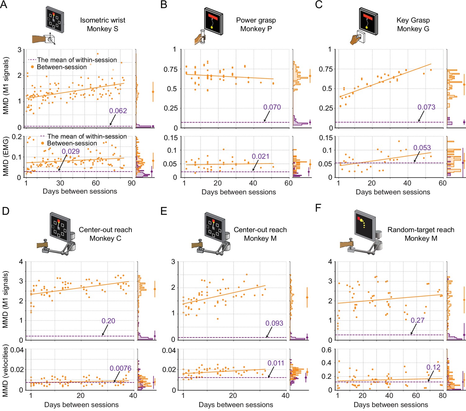
Evaluation of the stability of M1 neural signals and motor outputs over time for monkeys / tasks (besides monkey J).
Stability is characterized by the discrepancy in the distributions of signals between pairs of recording sessions in each dataset, which are measured by maximum mean discrepancy (MMD). Each subplot corresponds to a dataset: isometric wrist task of monkey S (A), power grasp of monkey P (B), key grasp of monkey G (C), center-out reach of monkey C (D) and monkey M (E), and random-target reach of monkey M (F). In each subplot, we showed the between-session MMD (orange) for M1 signals (top panel) and motor outputs (either EMG or hand velocity, bottom panel), and indicated the mean value of the within-session MMDs using a dashed purple line. The histograms for within-session and between-session MMDs are plotted on the right side of each panel, and the mean (solid dots) and standard deviation (solid lines) are shown.
Figure 2—figure supplement 4
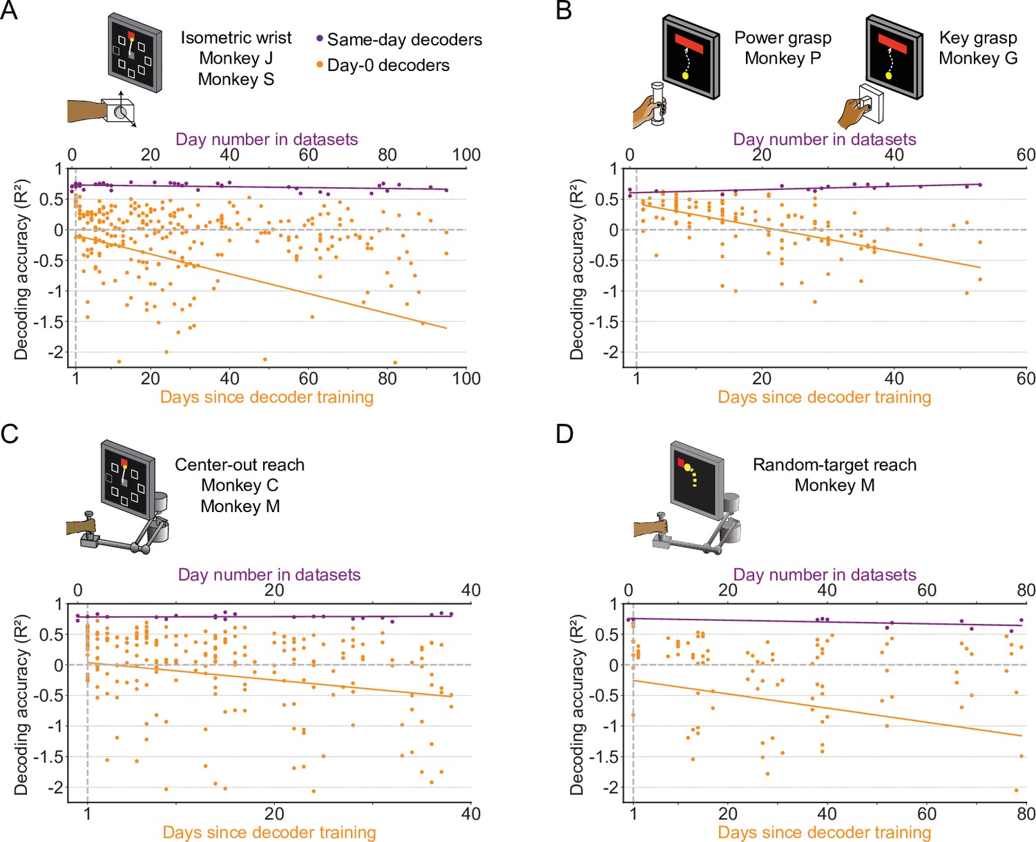
The accuracy of a well-calibrated iBCI decoder degrades over time for different behavioral tasks.
We fit an iBCI decoder (Wiener filter) using the data collected on a specific day (day-0), and used this decoder to predict the motor outputs from M1 signals for all remaining days in a dataset (day-k). The performance of the decoder was evaluated by the R² value between the actual signals and the predictions. We used all available days in a dataset as the day-0 and repeated the same analysis for them. Each subplot corresponds to a behavioral task, and may contain the data from multiple monkeys: isometric wrist task of monkeys J and S (A), power and key grasp of monkeys P and G (B), center-out reach of monkeys M and C (C), random-target reach of monkey M (D). In each subplot, the R² values when using decoders to predict the motor outputs on the same day they were fit are shown (same-day decoders, purple). The x-axis on the top shows the number of the day which the recording session is on, where “0” corresponds to the earliest date in a dataset. The R² values when using decoders to predict the motor outputs on day-k are also shown (day-0 decoders, orange). The x-axis on the bottom shows the days since decoder training. The solid lines show linear fits for the R²s of the same-day decoders (purple) and day-0 decoders on day-k (orange).
Figure 3 with 3 supplements
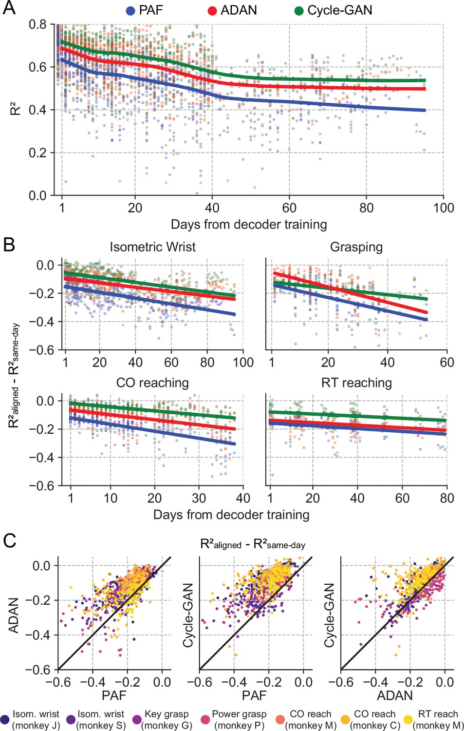
The proposed GANs-based domain adaptation methods outperform Procrustes Alignment of Factors in diverse experimental settings.
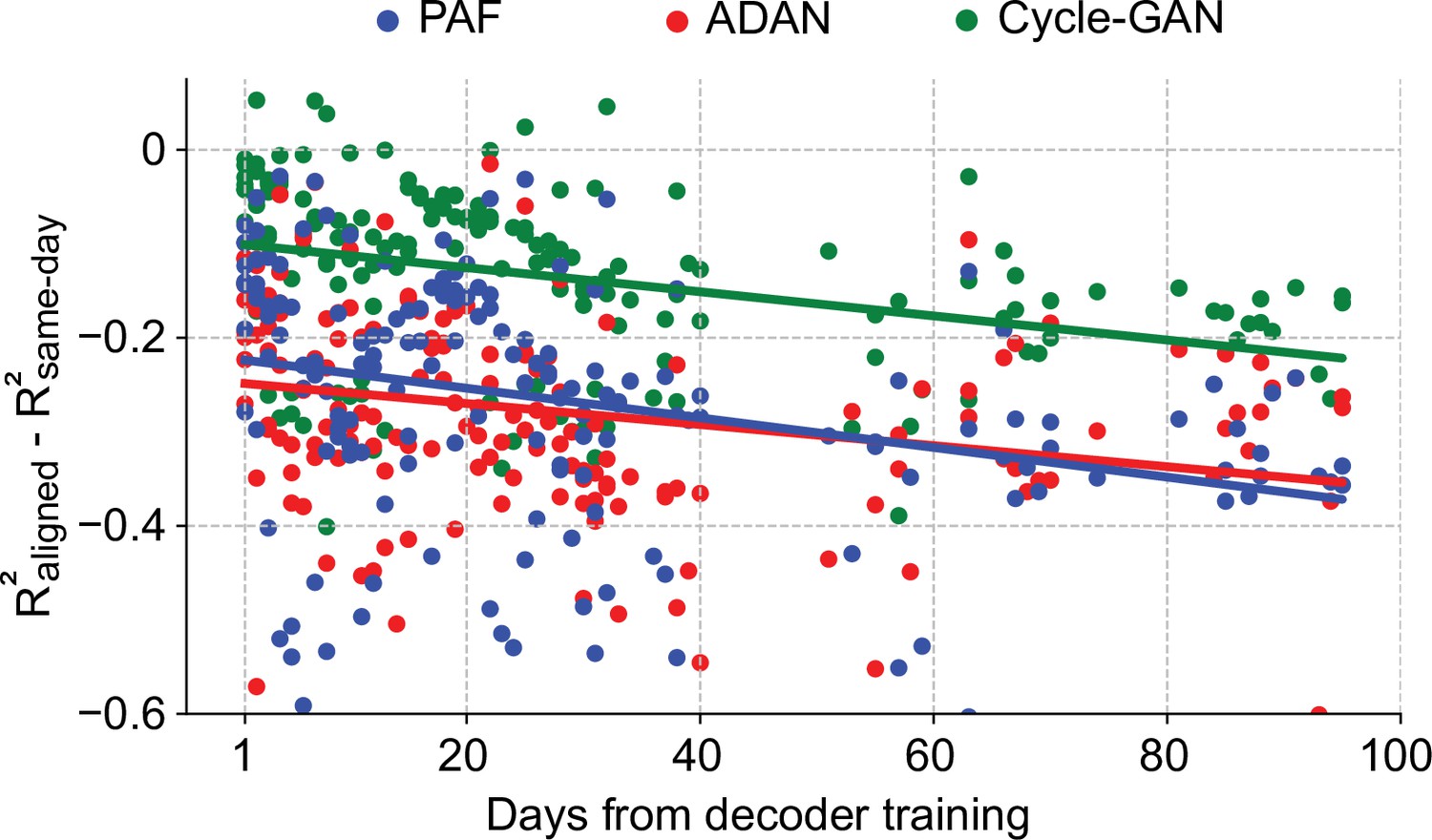
(A) Prediction accuracy over time using the fixed decoder trained on day-0 data is shown for all experimental conditions (single dots: R² as a function of days after decoder training, lines: locally weighted scatterplot smoothing fits). We compared the performance of the day-0 decoder after domain adaptation alignment with Cycle-GAN (green), ADAN (red) and PAF (blue). (B) We computed the prediction performance drop with respect to a daily-retrained decoder (single dots: R² drop (R²aligned - R²same-day) for days after decoder training, lines: linear fits). Cycle-GAN and ADAN both outperformed PAF, with Cycle-GAN degrading most slowly for all the experimental conditions. (C) We compared the performance of each pair of aligners by plotting the prediction performance drop of one aligner versus that of another. Each dot represents the R² drop after decoder training relative to the within-day decoding. Marker colors indicate the task. Both proposed domain adaptation techniques outperformed PAF (left and center panels), with Cycle-GAN providing the best domain adaptation for most experimental conditions (right panel).
Figure 3—figure supplement 1
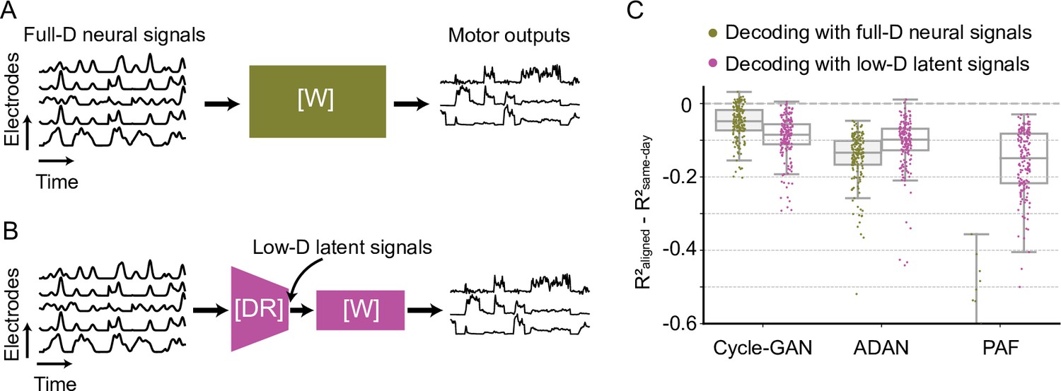
Cycle-GAN outperforms ADAN and Procrustes Alignment of Factors (PAF) with both full-dimensional and low-dimensional day-0 decoder.
We trained the day-0 decoders for each alignment method with either the full-dimensional firing rates (A) or the corresponding projections in a low-dimensional space (B). For the full-D decoder of ADAN and PAF, we used the reconstructed firing rates obtained from their nonlinear and linear latent space respectively. For ADAN, we used the decoder sub-network of the day-0 AE and for PAF we reversed the day-0 FA parameters to reconstruct the full-D firing rates. (C) Cycle-GAN outperforms ADAN and PAF with both a full-D (olive) and low-D (magenta) day-0 decoder. ADAN and PAF work better with a day-0 decoder trained on the latent signals. Note that PAF fails with a full-D decoder. For each alignment method, we computed the decoder performance drop with respect to a daily-retrained decoder (single dots: R² drop (R²aligned - R²same-day) for days after decoder training).
Figure 3—figure supplement 2
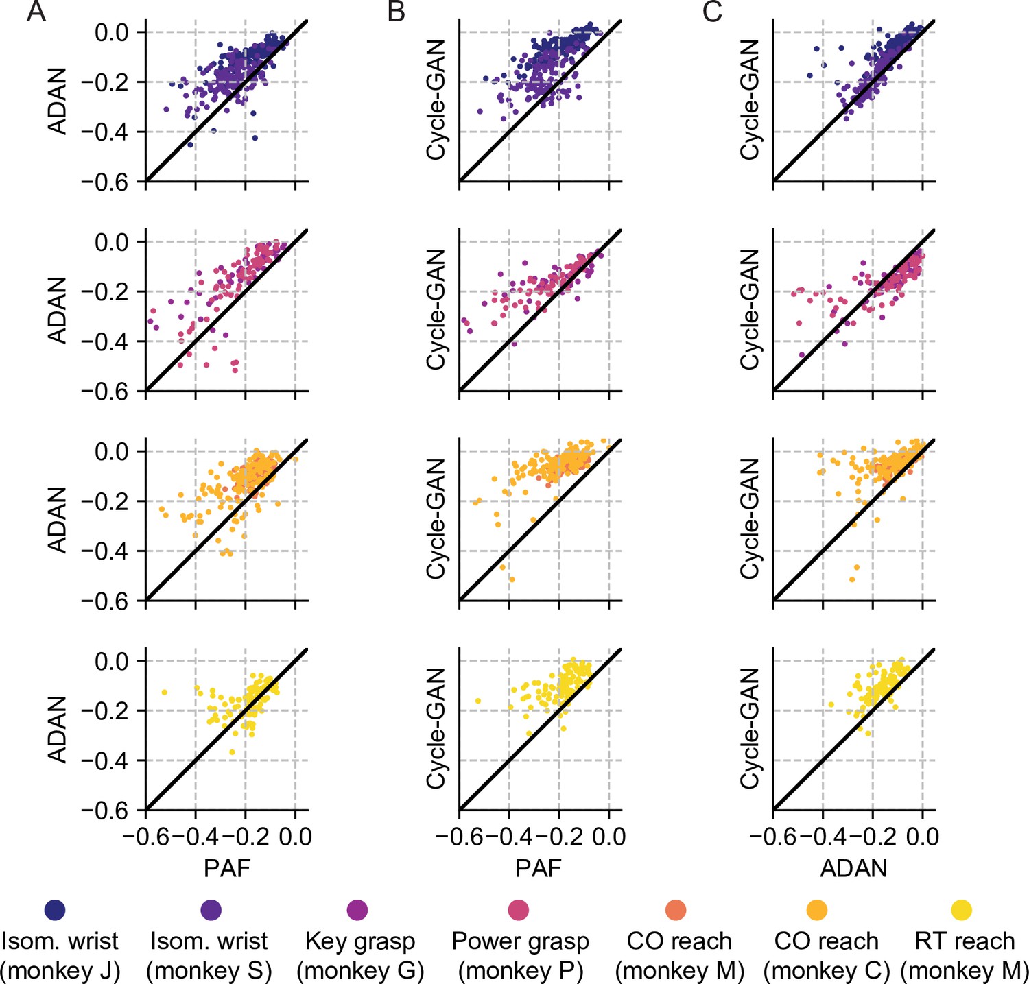
Cycle-GAN and ADAN consistently outperform Procrustes Alignment of Factors (PAF) for all experimental conditions.
(A) ADAN vs. PAF. (B) Cycle-GAN vs. PAF. (C) Cycle-GAN vs. ADAN. Figure shows the prediction performance drop with respect to a daily recalibrated decoder (R²aligned – R²same-day). Each dot represents the R² drop of a given day-k. Marker colors indicate the task. Points above the unity line indicate that the aligner on the y-axis outperformed that on the x-axis. ADAN and Cycle-GAN outperform PAF for both EMG (isometric wrist, 1st row and key/power grasping, 2nd row) and kinematic (center out reaching, 3rd row and random target reaching, 4th row) decoding. Cycle-GAN performances are slightly superior to those of ADAN for the tasks where we decoded EMG (1st and 2nd row). This difference was more remarkable for the tasks where we decoded hand velocity (3rd and 4th row).
Figure 3—figure supplement 3
Cycle-GAN outperforms ADAN and Procrustes Alignment of Factors (PAF) when aligning continuous neural recordings.
We compared the performance of the day-0 decoders, trained without excluding the inter-trial data, after domain adaptation alignment with Cycle-GAN (green), ADAN (red) and PAF (blue). We computed the prediction performance drop with respect to a daily-retrained decoder (single dots: R² drop (R²aligned - R²same-day) for days after decoder training, lines: linear fits). The accuracy of the fixed decoder on day-1 was significantly different across the aligners, with Cycle-GAN showing the least decoding drop, followed by ADAN and PAF. The performance degradation for periods greater than one day was mitigated in a similar way by all three alignment methods.
Figure 4
Cycle-GAN is more robust to hyperparameter tuning than ADAN.
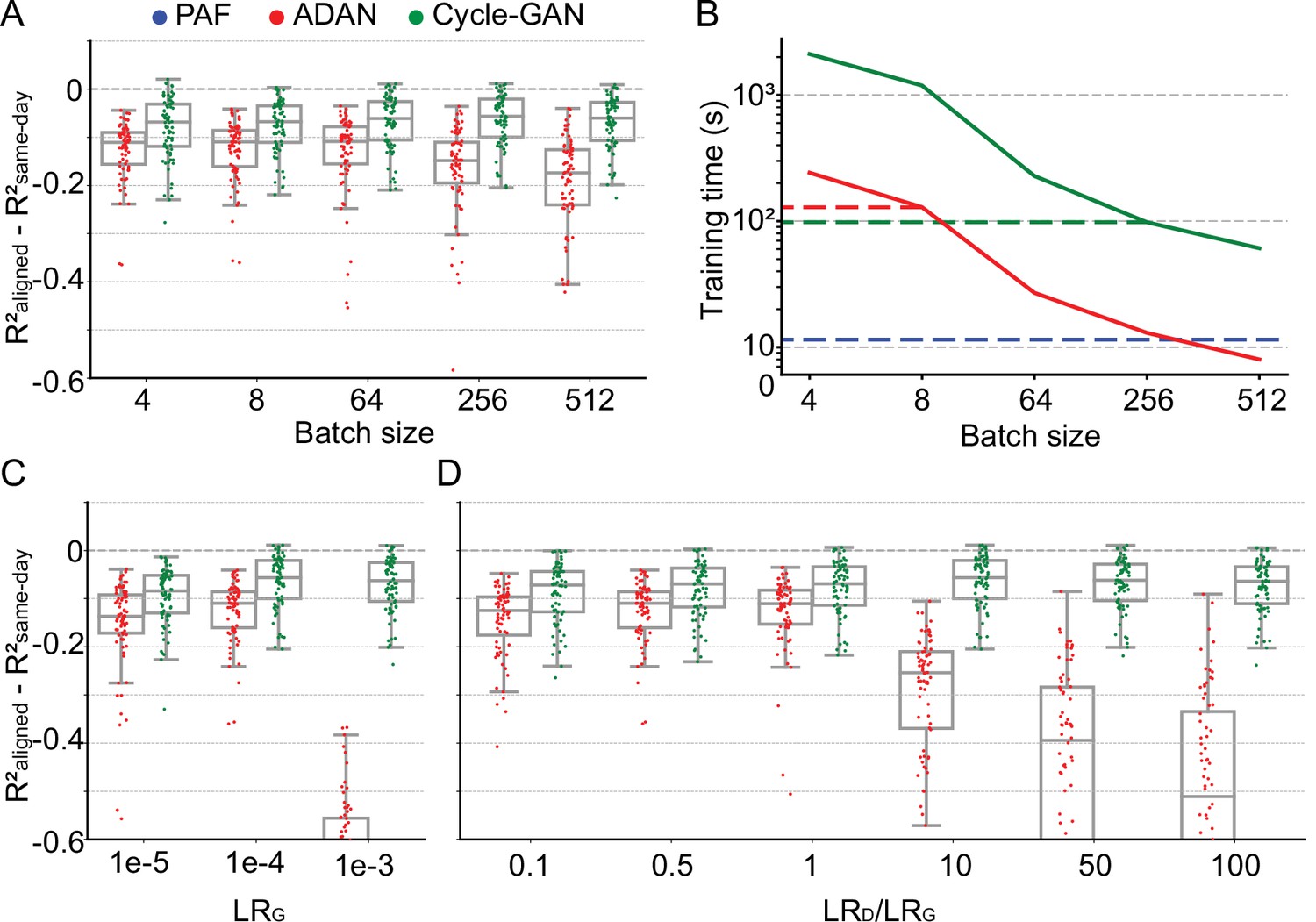
Effect of different batch sizes during training of Cycle-GAN (green) and ADAN (red) with mini-batch gradient descent on (A) the day-k performance of 4 selected day-0 decoders and (B) the execution time of 200 training epochs. The much faster execution time of PAF (blue) is also shown for reference. Compared to ADAN, Cycle-GAN did not require a small batch size, resulting in faster training (Cycle-GAN: 98 s with batch size 256; ADAN: 129 s with batch size 8; FA aligner: 11.5 s). Effect of training each domain adaptation method with different generator (C) and discriminator (D) learning rate. The generator and the discriminator learning rate were denoted as LRG and LRD, respectively. For LRD testing, we kept LRG fixed (LRG = 1e-4 for both ADAN and Cycle-GAN), and changed the ratio between LRD and LRG (LRD/LRG). ADAN-based aligners did not perform well for large LRG or LRD/LRG values, while Cycle-GAN-based aligners remained stable for all the testing conditions. In (A), (C) and (D) single dots show the prediction performance drop on each day-k relative to the 4 selected day-0s with respect to the R² of a daily-retrained decoder (R²aligned - R²same-day). Boxplots show 25th, 50th and 75th percentiles of the R² drop with the whiskers extending to the entire data spread, not including outliers.
Figure 5
Cycle-GAN and ADAN need only a limited amount of data for training.
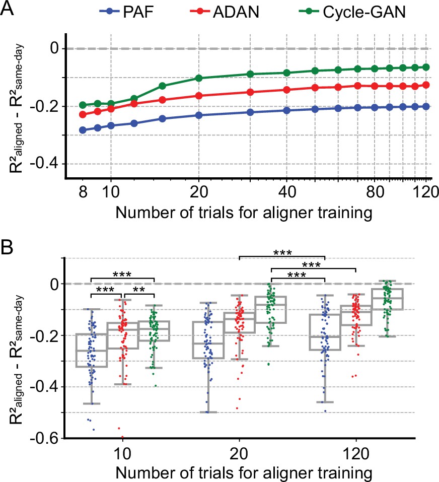
(A) Effect of the number of trials used for training Cycle-GAN (green), ADAN (red) and PAF (blue) on the day-k decoding accuracy using 4 selected day-0 fixed decoders. All the aligners needed 20–40 trials to achieve a satisfactory performance, before reaching a plateau. The average prediction performance drop with respect to a daily-retrained decoder (R²aligned - R²same-day) on all day-ks is shown for each tested value of training trials (x-axis is in log scale). When using 10 trials, both Cycle-GAN and ADAN significantly outperformed PAF (B, left boxplots). Moreover, both Cycle-GAN-based and ADAN aligners trained with 20 trials had significantly better performance than the PAF trained on all 120 trials (B, center and right boxplots). Single dots show the prediction performance drop on each day-k to the 4 selected day-0s with respect to a daily-retrained decoder. Boxplots show 25th, 50th and 75th percentiles of the R² drop with the whiskers extending to the entire data spread, not including outliers. Asterisks indicate significance levels: *p<0.05, **p<0.01, ***p<0.001.
Figure 6
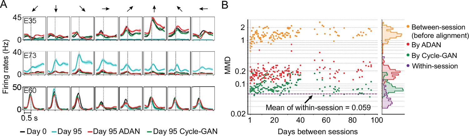
The changes of single-electrode and coordinated neural activity patterns after alignment.
(A) The PETHs of the multiunit activity from three cortical electrodes (E35, E73, E60) before and after alignment. Each column corresponds to a target direction indicated by the arrows on the top. For each direction, mean (solid lines) and standard errors (shaded areas) are shown for 15 trials. The dashed vertical line in each subplot indicates the time of force onset. (B) Between-session MMDs for M1 signals before and after alignment, as well as the within-session MMDs. The main panel plots the between-session MMDs before (orange) and after alignment (red: by ADAN, green: by Cycle-GAN) for all pairs of sessions with different days apart, and the dashed purple line indicates the mean of the within-session MMD values. The side panel plots the histogram for each type of data. Note y-axis is in log scale.
Figure 7
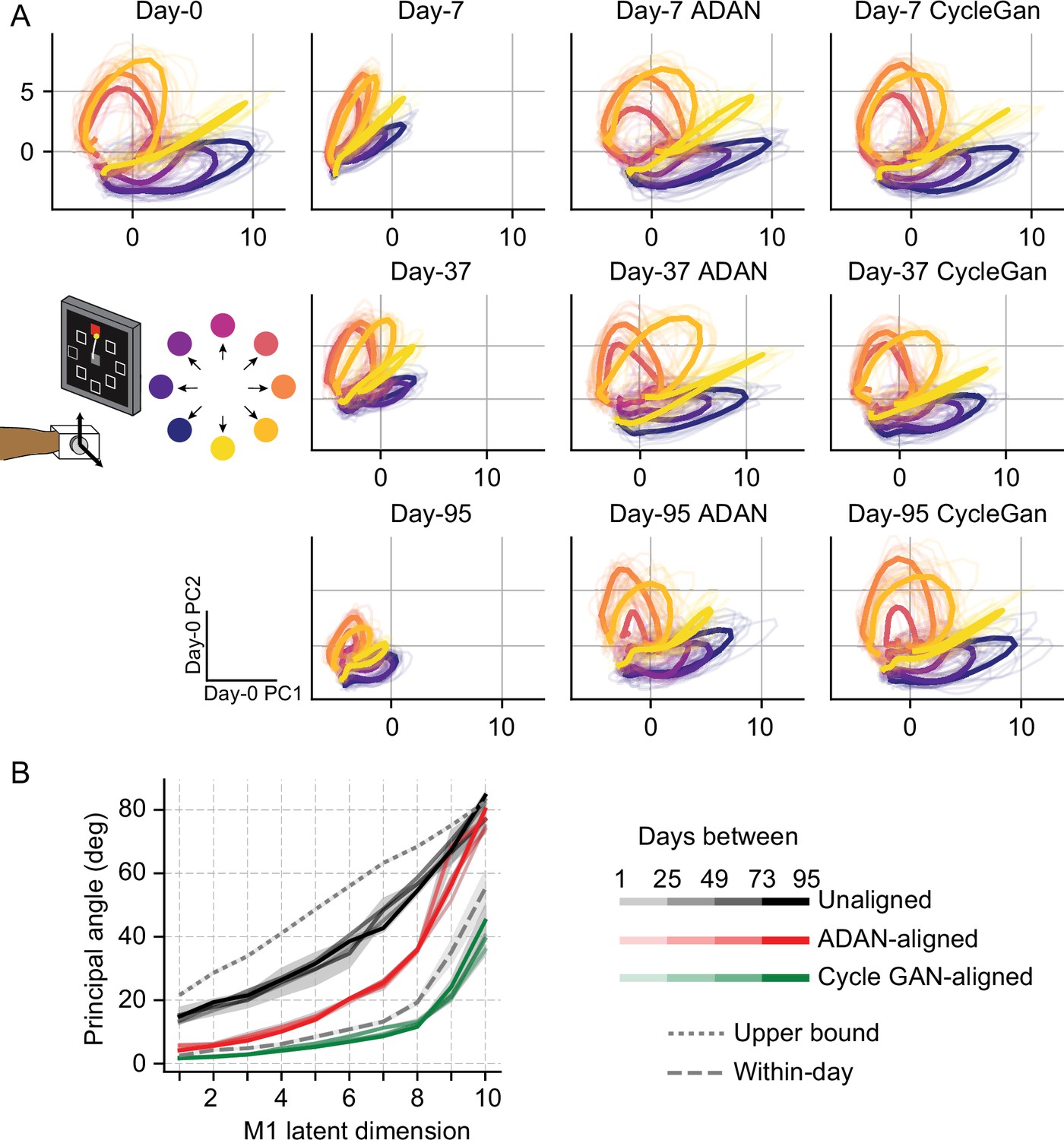
Neural manifold is stable over time after domain adaptation based neural alignment.
(A) Representative latent trajectories when projecting unaligned / aligned neural activity onto the first two principal components (PCs) for the day-0 neural activity of monkey J during isometric wrist task. Top left corner: latent trajectories for day-0 firing rates, as the reference. 2nd column: latent trajectories for unaligned firing rates on day-7 (top row), day-37 (center row) and day-95 (bottom row). 3rd column and 4th column: latent trajectories for firing rates aligned by ADAN (3rd column) and Cycle-GAN (4th column) on day-7, day-37, and day-95. Data were averaged over the first 16 trials for each target location and aligned to movement onset for visualization purposes. (B) First ten principal angles between the neural manifolds of day-0 and a given day-k for unaligned (black), aligned by ADAN (red) and aligned by Cycle-GAN (green). Upper bound was found by computing principal angles between surrogate subspaces with preserved statistics of day-0 and day-95 (0.1st percentile is shown). Within-day angles were found between subspaces relative to even-numbered and odd-numbered trials of day-0 neural recordings. Principal angle values were averaged across four different time intervals (relative to initial decoder training) indicated by the transparency of the line (lighter for days closer to day-0, darker for days further away from day-0).
Appendix 1—figure 1
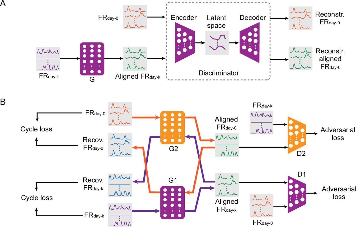
Adversarial neural networks proposed for iBCI stabilization.
(A) The architecture of ADAN. A feedforward network (the generator, ‘G’) takes the neural firing rates on day-k (‘FRday-k’) as input and applies a transform on them to produce the aligned neural firing rates (‘Aligned FRday-k’). Next, an autoencoder (the ‘Discriminator’) takes as input both the firing rates on day-0 (‘FRday-0’) and the Aligned FRday-k and aims to discriminate between them, giving the adversarial loss. (B) The architecture of CycleGAN used as an aligner for an iBCI. A feedforward neural network (‘G1’) takes FRday-k as input and produces Aligned FRday-k after applying a transformation. Another feedforward network (‘D1’) aims to discriminate between Aligned FRday-k and FRday-0; the performance of D1 contributes the first adversarial loss. A second pair of feedforward networks (‘G2’ and ‘D2’) function in the same way, but aim to convert FRday-0 into an Aligned FRday-0 that resembles FRday-k; these contribute to the second adversarial loss. The discrepancy between the real FRday-k and Recovered FRday-k (generated by passing FRday-k through G1 followed by G2) contributes a cycle loss (and similarly for FRday-0 and Recovered FRday-0). The purple and orange arrows highlight these two cyclical paths through the two networks.
Tables
Appendix 1—table 1
ADAN hyperparameters.
| parameter | value |
|---|---|
| Total number of trainable parameters | 35,946 |
| Batch size | 8 |
| Discriminator () learning rate | 0.00005 |
| Generator () learning rate | 0.0001 |
| Number of training epochs | 200 |
Appendix 1—table 2
Cycle-GAN hyperparameters.
| parameter | value |
|---|---|
| Total number of trainable parameters | 74,208 |
| Batch size | 256 |
| Discriminator () learning rate | 0.01 |
| Discriminator () learning rate | 0.01 |
| Generator () learning rate | 0.001 |
| Generator () learning rate | 0.001 |
| Number of training epochs | 200 |
Additional files
Download links
A two-part list of links to download the article, or parts of the article, in various formats.
Downloads (link to download the article as PDF)
Open citations (links to open the citations from this article in various online reference manager services)
Cite this article (links to download the citations from this article in formats compatible with various reference manager tools)
Using adversarial networks to extend brain computer interface decoding accuracy over time
eLife 12:e84296.
https://doi.org/10.7554/eLife.84296


