Error prediction determines the coordinate system used for the representation of novel dynamics
- Neuromuscular Diagnostics, TUM School of Medicine and Health, Department Health and Sport Sciences, Technical University of Munich, Germany
- Munich Institute for Robotics and Machine Intelligence (MIRMI), Technical University of Munich, Germany
- Munich Data Science Institute (MDSI), Technical University of Munich, Germany
Figures
Figure 1
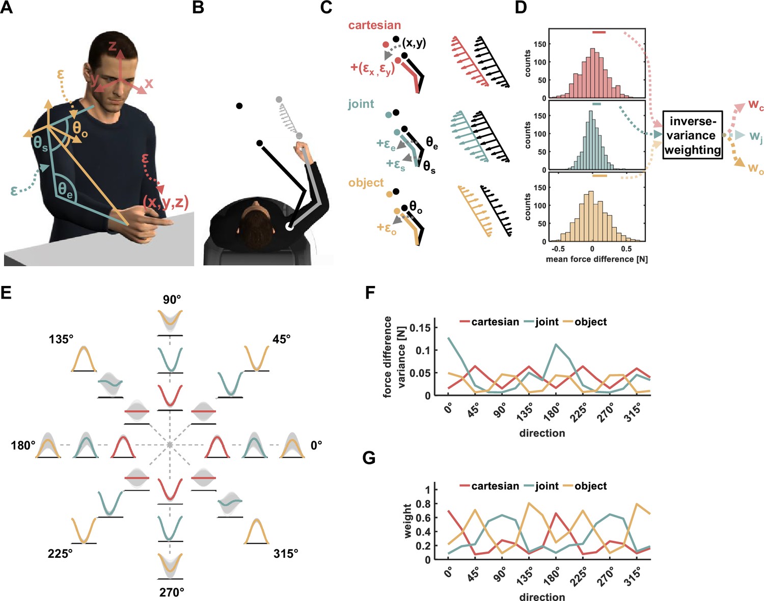
The Re-Dyn mechanism for representing dynamics.
(A) We considered three main types of coordinate systems for dynamics representation namely Cartesian (red), joint (turquoise), and object (yellow) based representations. Each coordinate system depends on the estimation of different state variables, which include joint angular values or hand coordinates, and those estimations can be distorted by neural noise (ε). (B) To test which coordinate system is used for dynamics representation we examined how learned dynamics are generalized in space. Participants moved between points in one position in space (gray circles) while experiencing external forces (gray arrows) and we examined the pattern of these forces in other locations in space using a force channel method. The movement in the new location (black circles) required participants to change the posture of their arms. (C) For movements in new locations (black circles), each coordinate system predicts a different pattern of generalized forces (black arrows pattern). These predictions are the desired generalized force pattern according to each reference frame and can be different due to the nature of each reference frame. However, since the current state of the arm has some uncertainties due to neural noise, ε, the spatial end-point position or arm orientation is incorrectly estimated (marked using gray arrows). As a result, the motor system might generate different pattern of forces compared to the pattern desired pattern. That is, noisy estimations for end point position (red), joints angles values (turquoise), and hand orientation value (yellow) in the new locations can alter the force pattern for the Cartesian, joint, and object-based representations, respectively. (D) Depending on the spatial location of the training and generalization movements, similar noise characteristics can have different effect sizes on the difference between desired and generated force patterns. This can be quantified by calculating the difference multiple times while randomizing the noise value. Based on the force difference distribution for each representation we can estimate the relative contribution of each representation to the generalized forces. This relative weight can be calculated using, for example, the inverse of the distribution variance. (E) An example for repeating the calculations for the Re-Dyn predicted weights across multiple directions. For each direction and according to each of the coordinate systems, we simulated distorted force patterns (gray curves) and compared them to the desired force profile marked using a colored curve (red-Cartesian, turquoise- joints, yellow- object). The distribution of the gray curves around the desired curve gives a sense of the distribution of error for each movement direction. (F) Based on the example in (E), we calculated the force difference variance of each coordinate system for each direction. To calculate this variance, we repeated the procedure in (D); that is, for each simulation (gray curve), we calculated the mean force difference from the desired force profile (colored curve). These differences were used to construct the mean force difference distribution and to calculate how variable this distribution is. (G) Using the variance profiles in (F) we calculated the weights using an inverse-variance formula (see Methods for more details).
Figure 2
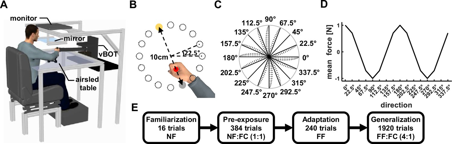
Experimental Design.
(A) Participants sat in front of a robotic manipulandum system (vBOT) while grasping the handle of the robot with their right hand. The participants’ arm was supported by an airsled system that reduced friction during movement. The virtual environment was projected on a mirror from a monitor mounted above the movement space. (B) Display of the virtual workspace. The participants’ hand was represented using a red cursor that was aligned with the hand position. The task was to move from the start point (gray circle) to the target point (yellow circle). The start and target points were always located on the diameter of a 10 cm diameter circle. There were 16 possible starting points spaced evenly on the circumference of the circle. On each trial, only one set of start and target points were presented. (C) Endpoint force profiles as a function of movement direction. The forces were calculated using a scaled curl force field. The force profile that appeared in each direction is illustrated from the center to the boundary of the circle. (D) Cosine representation of the mean forces of the scaled force field as a function of movement direction. Clockwise forces were set as positive and counterclockwise forces were set as negative. (E) Experimental protocol. Initial familiarization phase included 16 trials in which no force was applied to the hand (null field, NF condition). The pre-exposure phase included unconstrained movements (NF condition) and movements in a force channel (FC condition), with a ratio of 1:1 in all three workspaces. In the adaptation phase, participants performed the movements under the force field perturbation (FF condition) only in the training workspace. In the last phase, we tested generalization using force channel trials (FC) that were introduced randomly at the training and test workspaces while participants kept moving under force field perturbations (FF) only in the training workspace. The ratio between force field and force channel trials was 4:1.
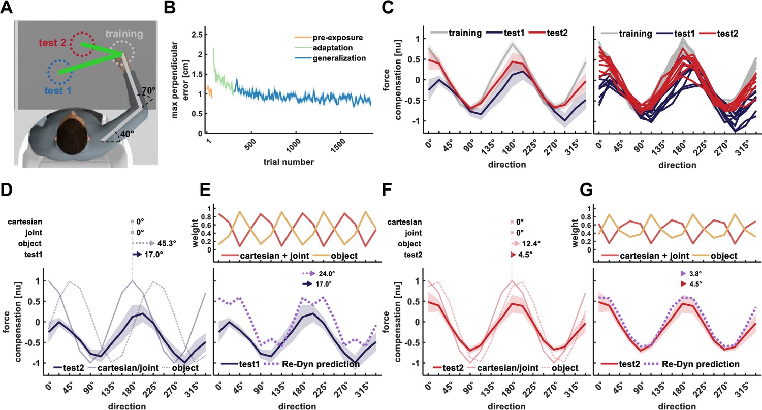
Figure 3
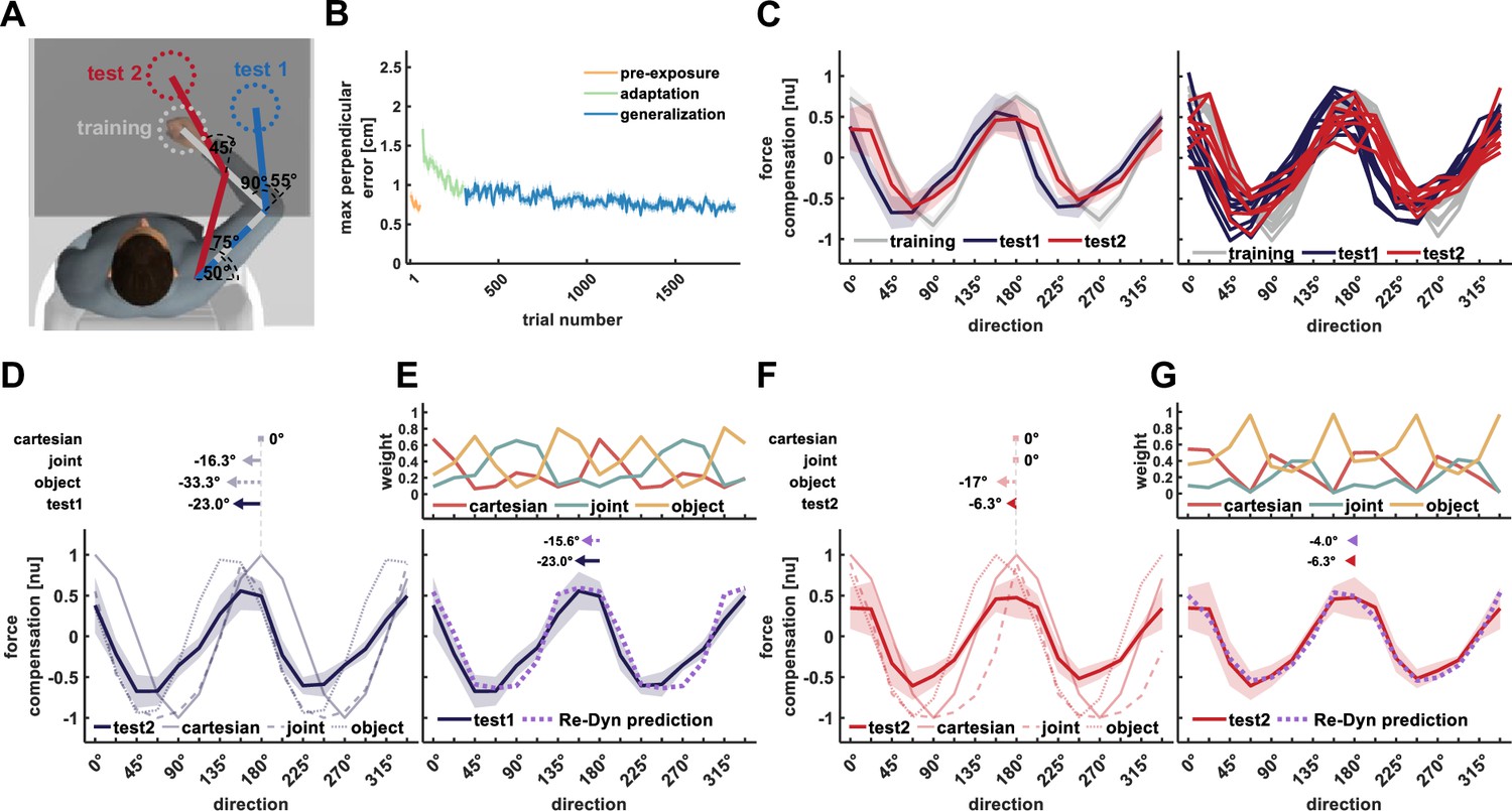
Results of experiment 1.
(A) Workspace locations for experiment 1. Participants adapted to the scaled curl force field in the training workspace (gray) while force generalization was tested in test workspace 1 (blue) and test workspace 2 (red). Each workspace location was set based on predefined values of shoulder and elbow joint angles and the measured length of the upper and forearm. Only the start and target locations for the current movement were displayed on each trial. (B) Mean maximum perpendicular error and standard error (shaded area) across participants during the pre-exposure phase (orange line), adaptation phase (green line), and generalization phase (blue line) of movements performed in the training workspace. (C) Left panel, mean force compensation profiles. Participants were able to adapt to the scaled force field as evidenced by the force compensation profile in the training workspace (gray curve) and showed a leftward shift of the curve for test workspace 2 (red curve) and more so for test workspace 1 (blue curve). Right panel, individual force compensation profiles for each participant in the different workspaces. (D) Mean force compensation profile for workspace 1 (dark blue solid line) and Cartesian (light blue solid line), joint- (light blue dashed line), and object- (light blue dotted line) based model predictions. Arrows above the panel indicate the shift of the mean force compensation profile and the models’ predictions with respect to the original curve describing the force field. (E) Upper panel, predicted weights for the Cartesian (red), joint- (turquoise), and object- (yellow) based representations for each movement direction according to the Re-Dyn model. Bottom panel, mean force compensation profile for workspace 1 (dark blue) and the predicted force compensation profile is generated by a mixture of reference frames according to the Re-Dyn predicted weights (purple). Arrows at the top indicate the shift of the mean force compensation profile and the model prediction. (F) Mean force compensation profile for workspace 2 (dark red solid line) and Cartesian (light red solid line), joint- (light red dashed line), and object- (light red dotted line) based model predictions. Arrows above the panel indicate the shift of the mean force compensation profile, similar to panel (D). (G) Upper panel, predicted weights for the mixture model, similar to panel (E). Bottom panel, mean force compensation profile for workspace 1 (dark red) and the Re-Dyn predicted force compensation profile (purple) similar to panel (E).
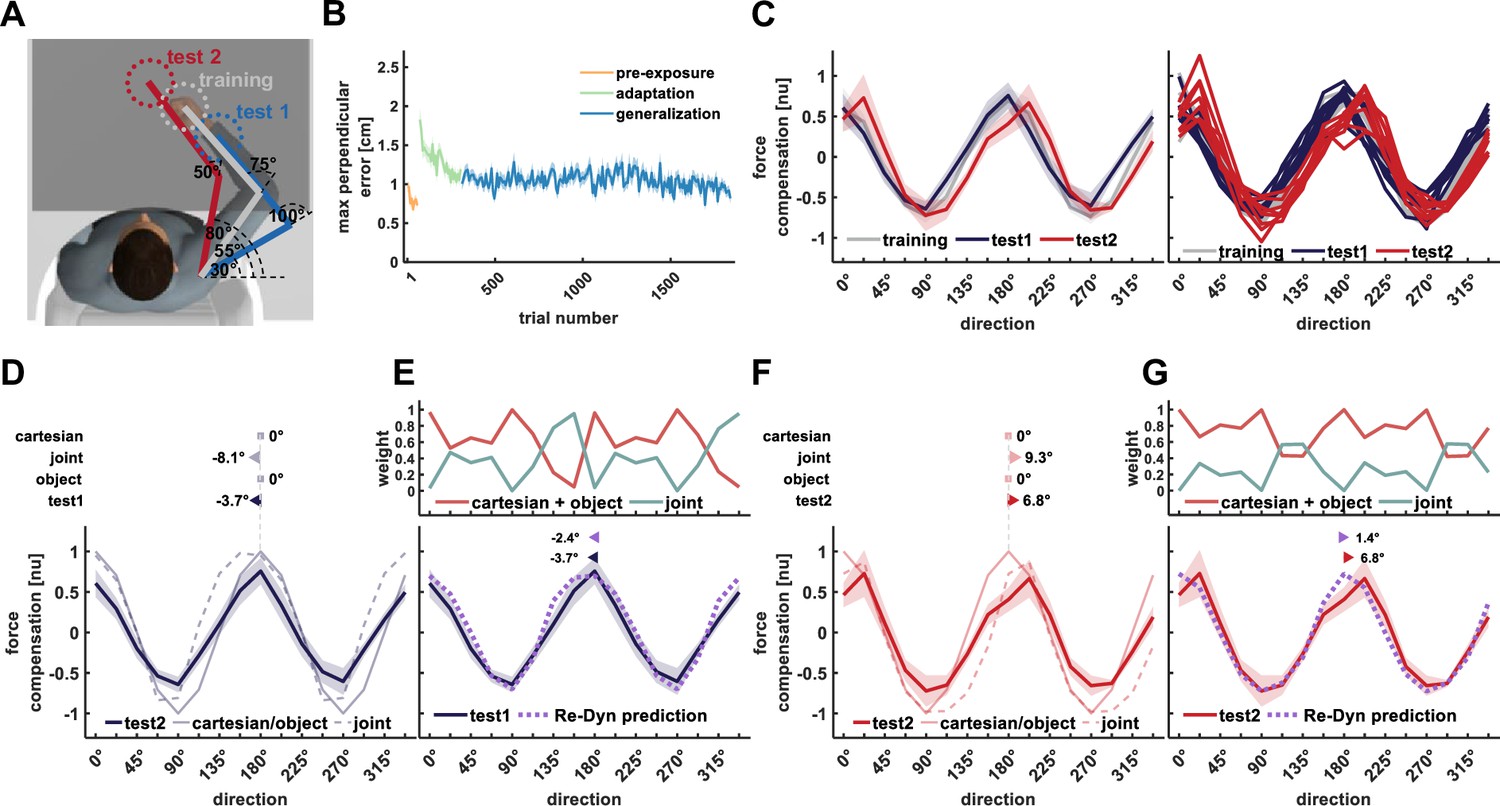
Figure 4
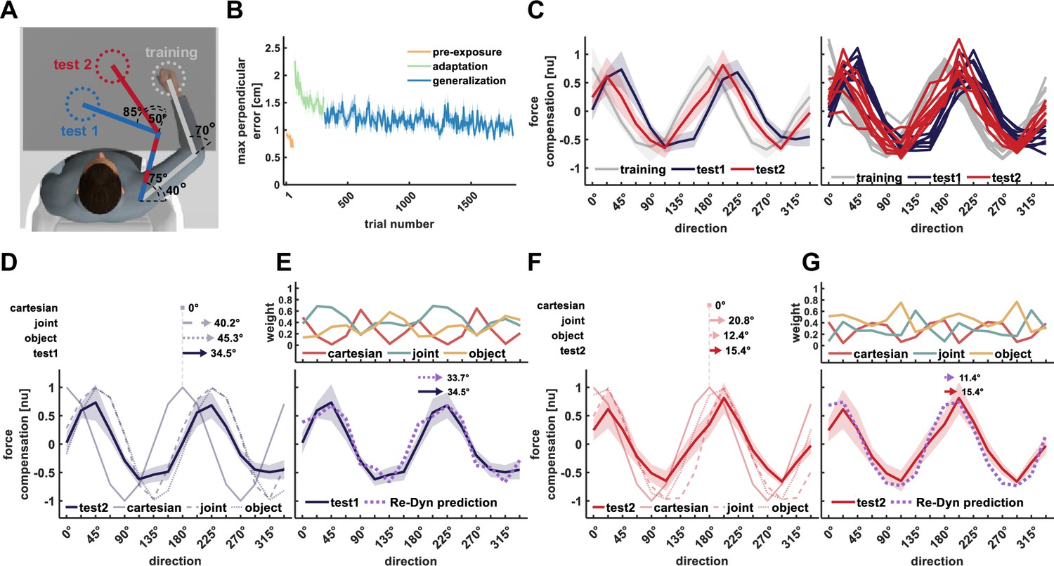
Results of experiment 2.
All notations are similar to Figure 3. (A) Workspace locations for experiment 2. (B) Mean maximum perpendicular error (MPE). (C) Left panel, mean force compensation profiles in the training and test workspaces. Right panel, individual force compensation profiles in the training and test workspaces. (D) Mean force compensation profile for workspace 1 and model predictions (same as Figure 3D). Arrows above the panel indicate the shift of the mean force compensation profile and the models’ predictions with respect to the original curve describing the force field. (E) Upper panel, the predicted weights for the mixture model for each movement direction according to the Re-Dyn model. Bottom panel, the resulted predicted force compensation profile generated by a mixture of reference frames (same as Figure 3E). Arrows at the top indicate the shift of the mean force compensation profile and the model prediction. (F) Mean force compensation profile for workspace 2 and model predictions (same as Figure 3F). Arrows above the panel indicate the shift of the mean force compensation profile and the models’ predictions with respect to the original curve describing the force field. (G) Upper panel, the predicted weights according to the Re-Dyn model. Bottom panel, the resulted predicted force compensation profile is generated by a mixture of reference frames, the same as panel (E).
Figure 5
Results of experiment 3.
All notations are similar to Figure 3. (A) Workspace locations. The participants always moved in the training workspace and the generalized forces were measured during movement of the endpoint of a pole (visually attached to the hand) in the same test workspaces as in experiment 2. (B) Mean maximum perpendicular error (MPE). (C) Left panel, mean force compensation profiles in the training and test workspaces. Right panel, individual force compensation profiles in the training and test workspaces (same as Figure 3C). (D) Mean force compensation profile for workspace 1 and model predictions (same as Figure 3D). Arrows above the panel indicate the shift of the mean force compensation profile and the models’ predictions with respect to the original curve describing the force field. (E) Upper panel, the predicted weights for the mixture model for each movement direction according to the Re-Dyn model. In this case, since the Cartesian and joint-based generalized forces are identical, their weight is equal and thus we used a sum of the two weights (Cartesian +joint). Bottom panel, the resulted predicted force compensation profile is generated by a mixture of reference frames (same as Figure 3E). Arrows at the top indicate the shift of the mean force compensation profile and the model prediction. (F) Mean force compensation profile for workspace 2 and model predictions (same as Figure 3F). Arrows above the panel indicate the shift of the mean force compensation profile and the models’ predictions with respect to the original curve describing the force field. (G) Upper panel, the predicted weights according to the Re-Dyn model. Bottom panel, the resulted predicted force compensation profile is generated by a mixture of reference frames, the same as panel (E).
Figure 6
Results of experiment 4.
All notations are similar to Figure 3. (A) Workspace locations for experiment 4. (B) Mean maximum perpendicular error (MPE). (C) Left panel, mean force compensation profiles in the training and test workspaces. Right panel, individual force compensation profiles in the training and test workspaces. (D) Mean force compensation profile for workspace 1 and model predictions (same as Figure 3D). Arrows above the panel indicate the shift of the mean force compensation profile and the models’ predictions with respect to the original curve describing the force field. (E) Upper panel, the predicted weights for the mixture model for each movement direction according to the Re-Dyn model. Bottom panel, the resulted predicted force compensation profile generated by a mixture of reference frames (same as Figure 3E). Arrows at the top indicate the shift of the mean force compensation profile and the model prediction. (F) Mean force compensation profile for workspace 2 and model predictions (same as Figure 3F). Arrows above the panel indicate the shift of the mean force compensation profile and the models’ predictions with respect to the original curve describing the force field. (G) Predicted weights the resulted predicted force compensation profile generated by a mixture of reference frames, same as panel (E).
Figure 7
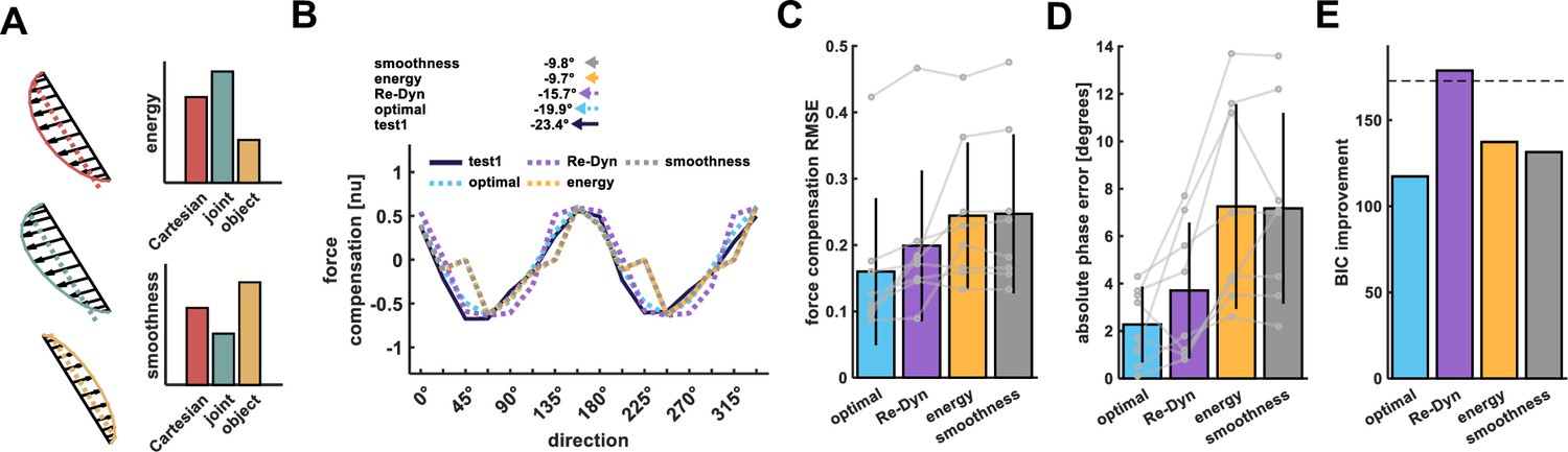
Comparison of prediction performance between Re-Dyn, energy, and smoothness-based models.
(A) An example for combining the Cartesian, joint, and object reference frames force profiles using minimum energy or maximum smoothness criteria. Using the predicted force profiles of each reference frame we calculated the energy (dashed line) and smoothness of the signal envelope (solid line). In this example, the energy required to produce the generalized forces is the smallest for the object-based coordinate system (yellow) followed by the Cartesian (red) and joint (turquoise) coordinate systems. Similarly, the generalized force profile according to the object coordinate system is smoother compared with the other coordinate systems. Thus, in this example, the object-based coordinate system will have an elevated weight compared with the other coordinate systems according to both the minimum energy model and maximum smoothness model. (B) Example for the Re-Dyn (purple dashed line), energy (yellow dashed line), and smoothness- (gray dashed line) based models force compensation predictions for the experimental force compensation curve exhibited by participants in experiment 1 while moving in test workspace 1 (blue solid line). The weights between coordinate systems for the optimal fit (light blue dashed line) were calculated based on minimizing the error between the experimental curve and the fitted curve. Arrows at the top of the panel indicate the shift of the mean force compensation profile and the models’ predictions with respect to the original curve describing the force field. (C) Bars represent the mean root mean square error (RMSE) between the predicted/fitted and experimental force compensation curves across all experiments. Error bars represent the standard deviation (n=8). Gray points represent individual RMSE values for each of the eight test workspaces we had in the four experiments. Lines connect the predictions/fitting for each test workspace. (D) Same notation as in C but for the mean phase shift error between the experimental force compensation profiles and the phase shift of the models’ predictions. (E) BIC Improvement for each of the models relative to no generalization (that is, a model in which the force is zero at all movement directions). Dashed line shows the cutoff for models that are not considered distinguishable in terms of their performance from the best model (Re-Dyn model).
Figure 8
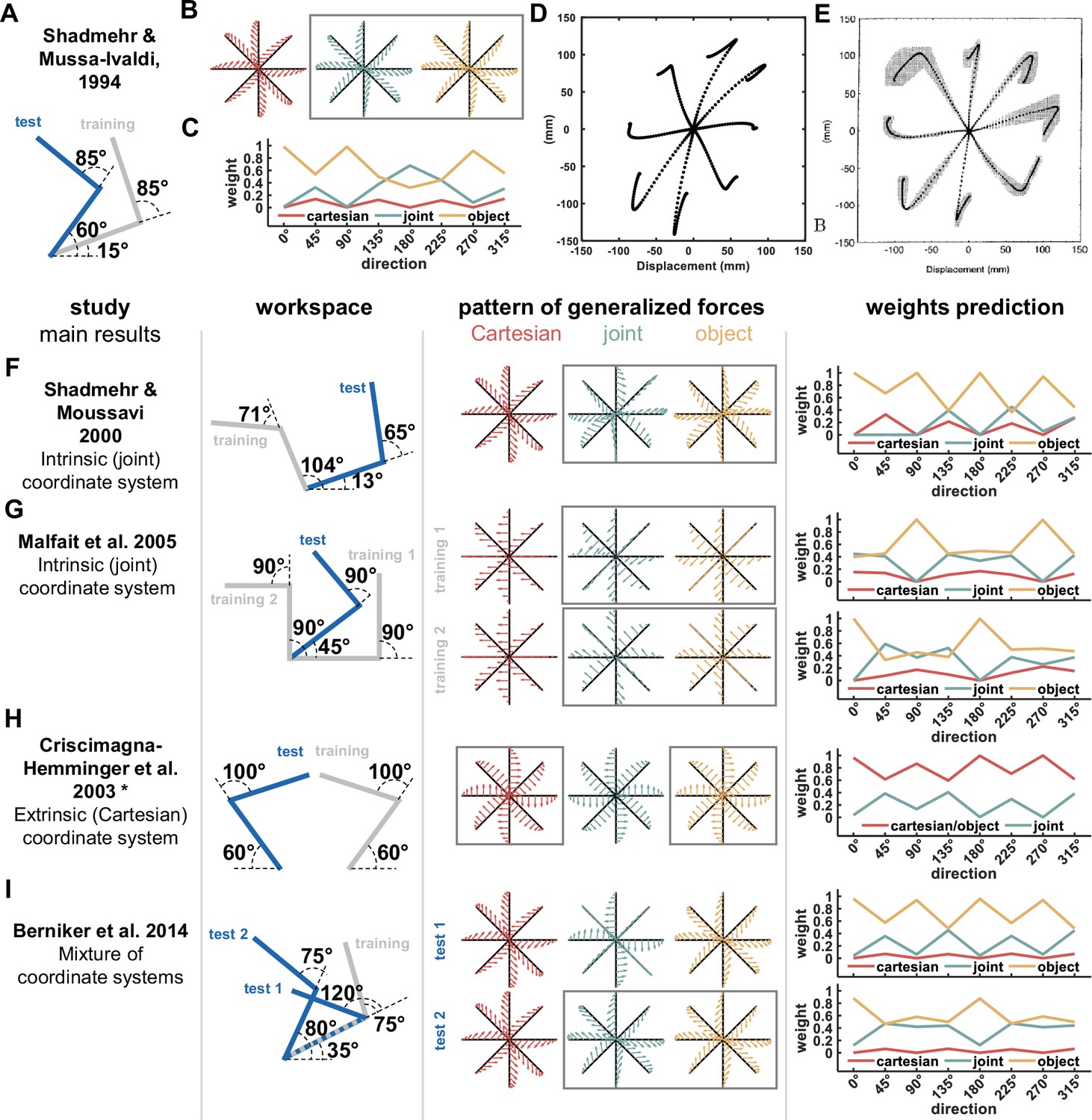
Predictions of the Re-Dyn model for weighting between coordinate systems for previous studies.
(A) Workspaces locations for the study by Shadmehr and Mussa-Ivaldi, 1994. (B) Pattern of generalized forces for the Cartesian (red), joint (turquoise), and object (yellow) coordinate systems. Arrows mark the direction and magnitude of each coordinate system predicted forces after adapting to a skew force field that was used in the original study. In this case, the joint and object-based coordinate system predict similar pattern of generalized forces (marked using a gray rectangle). (C) For the workspaces in (A), we calculated the Re-Dyn predicted weights between coordinate systems used for dynamic generalization. (D) We used an internal model which generates movements in free space after adaptation to the skew force field similar to the internal model used in the original study. In this case, since there are no external forces, we observed the after-effect movement pattern, i.e., movements that deviate from the straight line path due to counteractive forces produced by the internal model. The internal model uses a weighted sum of the three coordinate systems, Cartesian, joint, and object to generate these forces according to the weights in (C). Dashed lines represent paths to eight equally spaced targets from a center initial point. (E) Experimental results of the after-effect movements in the test workspace. The simulation results in (D) capture the deviation direction from the straight-line path, explaining how different coordinate systems were combined in this experiment. Moreover, since the joint and object coordinate systems predict the same pattern of generalized movement as well as they are the dominant systems in this representation, it can explain why the authors of the original study concluded that dynamic generalization is achieved using the joint coordinate system. Figure 8E is reproduced from Figure 14B from Shadmehr and Mussa-Ivaldi, 1994. (F–I) Predictions of the dominant reference frame according to the Re-Dyn model for previous experimental designs and comparison of these predictions with the conclusions of these past studies. Each row of panels includes the information presented in panels A-C for different studies. From left to right, panels present the main result of the study regarding the dominant coordinate system for dynamic representation, hand configuration used in the study setting the training and test workspaces locations, predicted generalized force patterns, and the simulated weights according to our Re-Dyn model. For the last panel, the simulated weights for Cartesian, joint, and object-based representations are marked using red, turquoise, and yellow lines, respectively. * In the original paper the authors did not mention the exact shoulder and elbow joints values, but instead mentioned that the arms were symmetric about the midline and workspaces were close to the midline. We estimated the configuration based on the sketch in Figure 1 in the original paper.
© 1994, Society for Neuroscience. Figure 8E is reproduced from Figure 14B from Shadmehr and Mussa-Ivaldi, 1994, with permission from Society for Neuroscience. It is not covered by the CC-BY 4.0 licence and further reproduction of this panel would need permission from the copyright holder.
Appendix 1—figure 1

Bayesian Information Criterion (BIC) Improvement for each of the models relative to no generalization (that is, a model in which the force is zero in all movement directions).
The dashed horizontal line shows the cutoff for models that are not considered distinguishable in terms of their performance from the best model.
Appendix 2—figure 1
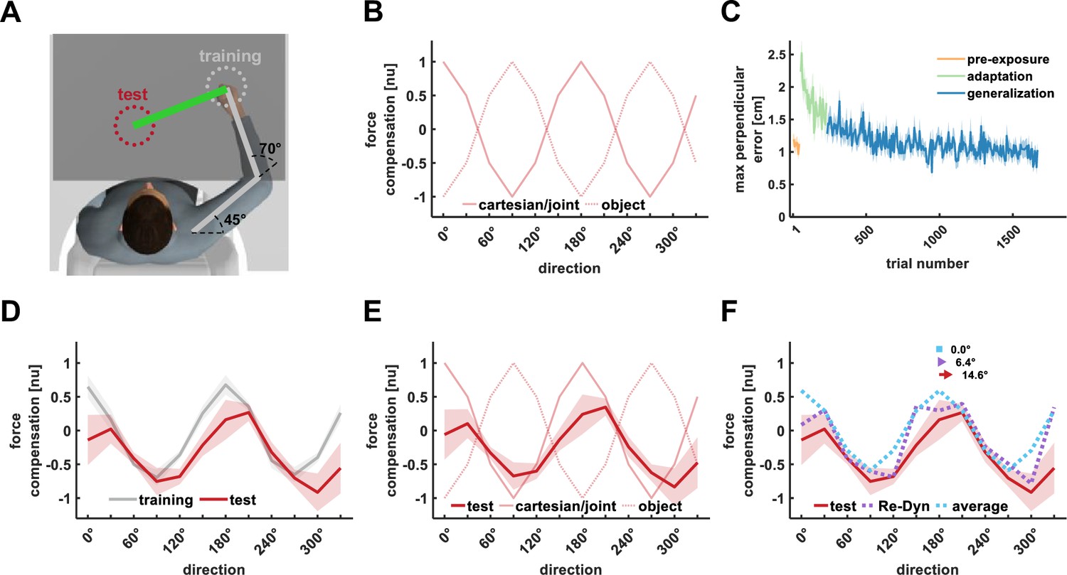
Direction-independent weights experiment.
(A) Similar to experiment 3, the participants moved in the training workspace and the generalized forces were measured during movement of the endpoint of a 90° rotated pole in a test workspace. (B) Predicted generalized force compensation patterns for the Cartesian/joint (solid line) and object-based (dotted line) coordinate systems for the test workspace.(C) Mean maximum perpendicular error (MPE) reduction during adaption to the trigonometric scaled force field. (D) Mean force compensation patterns and standard error (shaded area) in the training (gray) and test (red) workspaces. For the test workspace, the generalization pattern was shifted by 14.6°. (E) Mean force compensation profile for the test workspace (red solid line) and Cartesian/ joint- (light red solid line), and object- (light red dotted line) based model predictions. (F) Mean force compensation profile for the test workspace (red). To explain this pattern, we calculated the predicted force compensation profile generated by a mixture of reference frames according to the Re-Dyn predicted weights (purple dotted line) and a model based on direction-independent weights (light blue dotted line). In this case, the direction-independent weights model was calculated by setting equal weights between the three reference frames. Arrows at the top indicate the shift of the mean force compensation profile and the model’s prediction.
Author response image 1

Detailed simulation of weights for experiment 1, workspace 1.
Author response image 2

Weights of a random weights model.
Author response image 3

RMSE analysis comparing global fitted optimal model, three prediction based models, and a random weights model.
Author response image 4
Weights according to minimum energy model.
Author response image 5

Weights according to maximum smoothness model.
Additional files
Download links
A two-part list of links to download the article, or parts of the article, in various formats.
Downloads (link to download the article as PDF)
Open citations (links to open the citations from this article in various online reference manager services)
Cite this article (links to download the citations from this article in formats compatible with various reference manager tools)
Error prediction determines the coordinate system used for the representation of novel dynamics
eLife 14:e84349.
https://doi.org/10.7554/eLife.84349


