Spike-phase coupling patterns reveal laminar identity in primate cortex
- The Salk Institute for Biological Studies, United States
- Department of Neuroscience, Washington University in St. Louis School of Medicine, United States
- Department of Mathematics, Western University, Canada
- Brain and Mind Institute, Western University, Canada
Figures
Figure 1 with 2 supplements
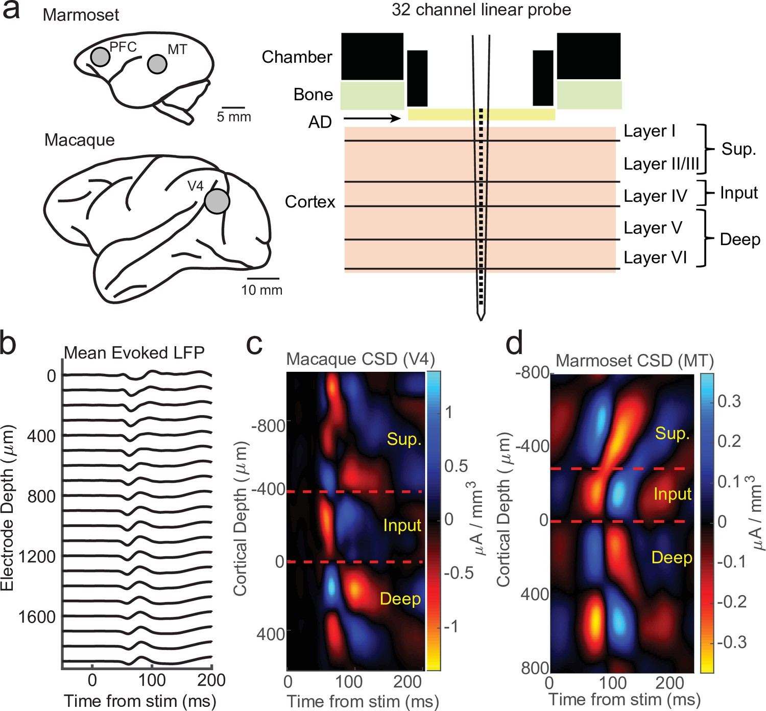
Current-source density (CSD) analysis reveals laminar boundaries in cortical recordings.
(a) Schematic of recording locations in two marmosets (PFC or MT) and two macaques (V4). Recordings were made with a 32-channel linear silicon probe in an acute recording chamber penetrating through a silicone artificial dura (AD). (b) Average evoked local field potential (LFP) responses to a stimulus flash (N = 141 trials) in an example macaque recording session in area V4. Each line is the response measured on a single contact. The depth is in absolute distance from the most proximal contact. (c) CSD measurement from the example recording session in b. The input layer is defined as the bottom and top of the earliest current sink (red), with the superficial and deep layers defined as above and below the input layer, respectively. Depth is measured relative to the bottom of the input layer. (d) Same as c, but in an example marmoset MT recording session (N = 225 trials).
Figure 1—figure supplement 1
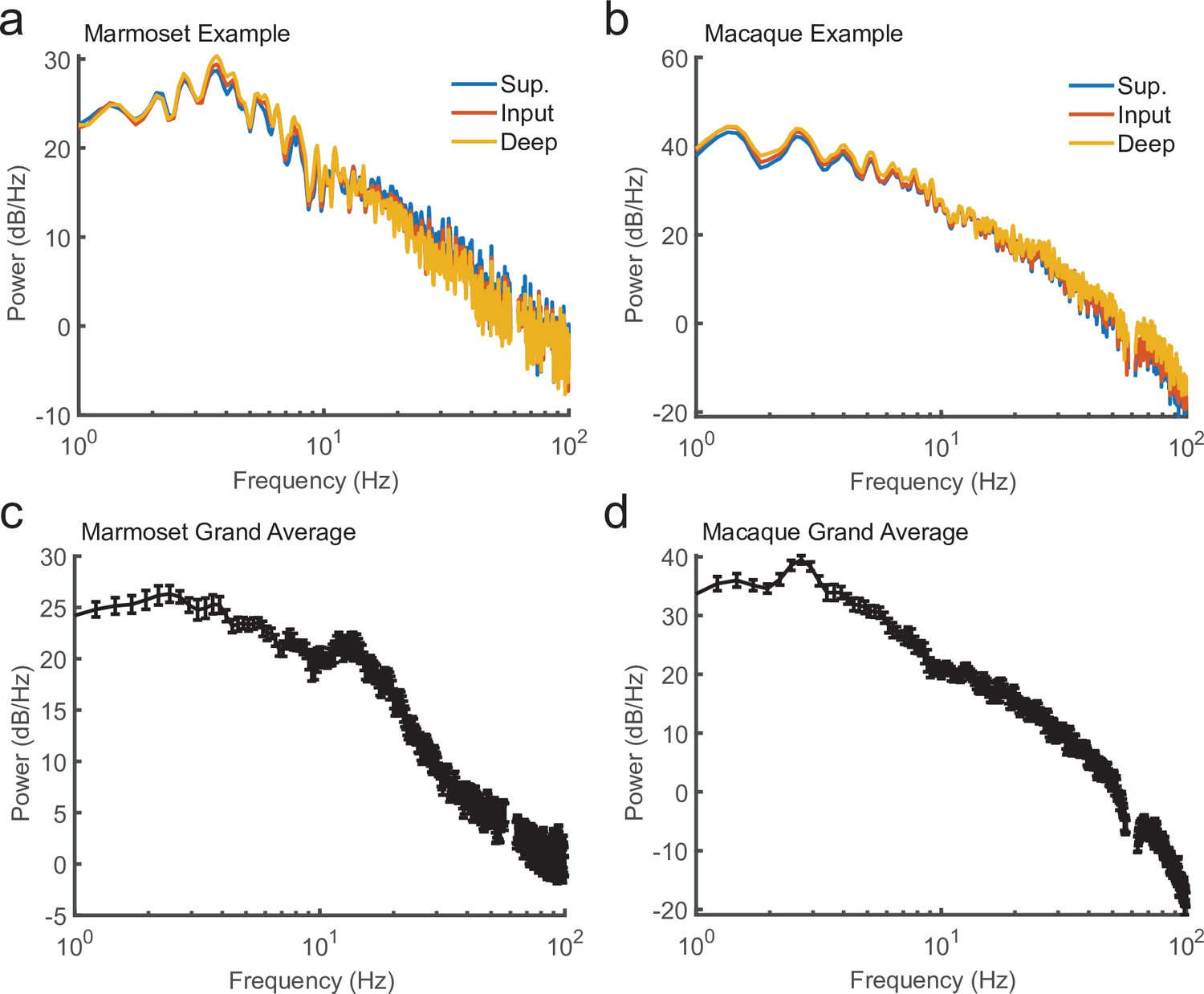
Power spectra of local field potential (LFP) recorded during current-source density (CSD) mapping.
(a) Power spectral density for 10 s of continuous LFP recorded from a marmoset during CSD mapping. Plotted are the power spectral density (PSD) from three channels based on their laminar compartment (superficial layers, blue; input layer, red; deep layers, yellow). (b) Same as in a, but from a macaque recording. (c) The average PSD for 10-s segments across all recording sessions in a single marmoset (N = 8; error bars denote standard error of the mean [SEM]). (d) Same as c, but for the sessions across one macaque (N = 6).
Figure 1—figure supplement 2
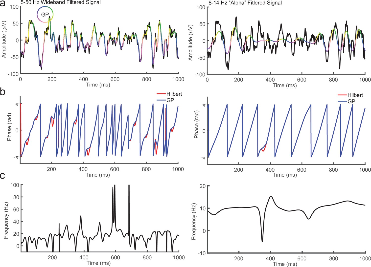
Comparison between Generalized Phase (GP) and Hilbert Transform for broad (5–50 Hz) and narrow (8–14 Hz) filtered signals.
(a) One second of local field potential (LFP; black) overlaid with the signal after filtering from 5 to 50 Hz (left) or alpha band (8–14 Hz, right). In pseudo color is the phase of the filtered signal using GP. (b) Comparison between phase measured using the Hilbert Transform (red line) and GP (blue line) for the 1 s 5–50 Hz (left) or 8–14 Hz (right) filtered LFP in a. (c) Instantaneous frequency of the 5–50 Hz (left) or 8–14 Hz (right) filtered LFP. Note the phase reversals for the Hilbert Transform in b occur where the instantaneous frequency becomes negative. These are targeted and replaced by the GP algorithm.
Figure 2
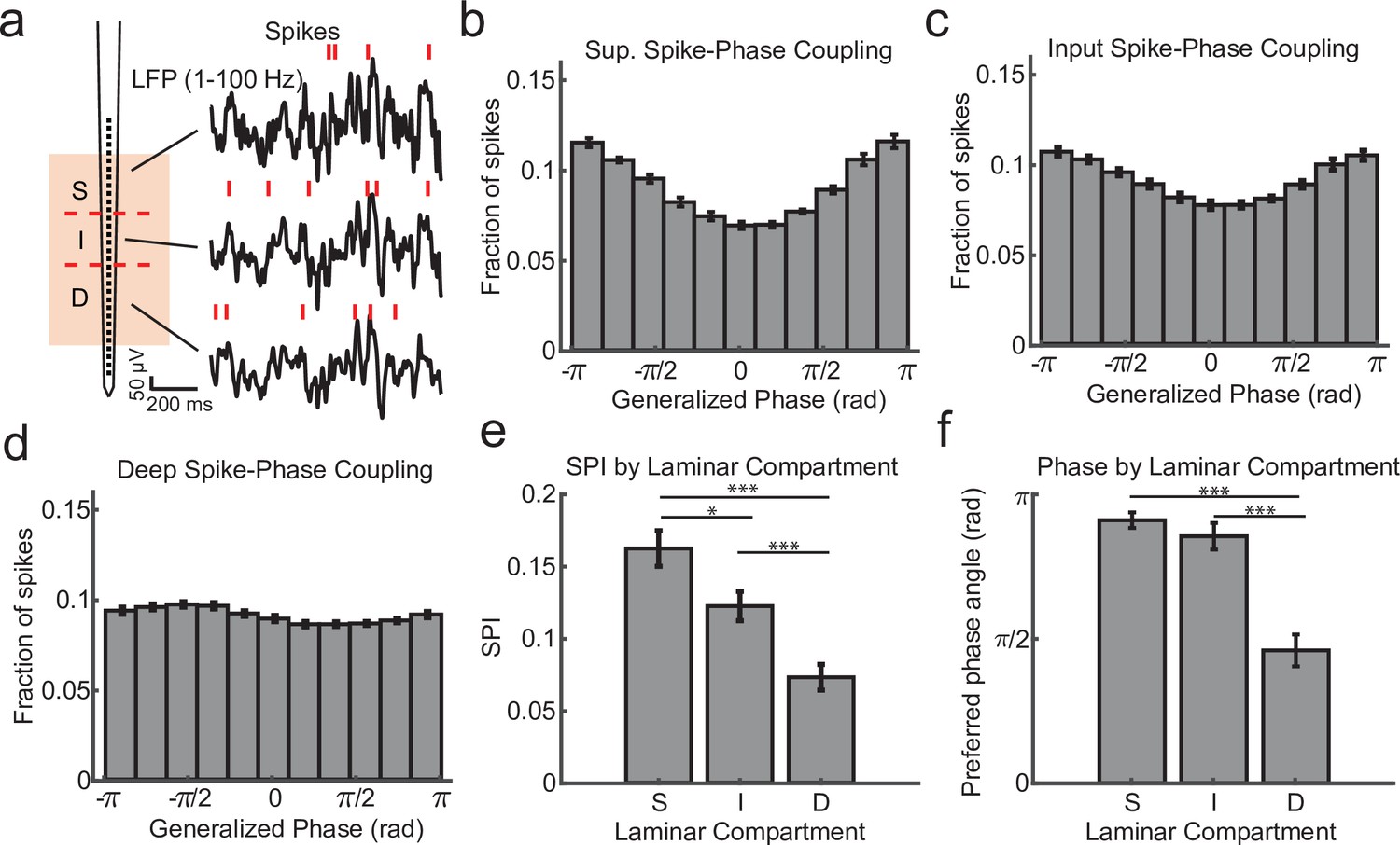
Within channel spike–local field potential (LFP) phase coupling strength and preferred phase angle varies across layers.
(a) Spike–LFP phase coupling was measured by taking the phase of the LFP on a contact at the times when multi-unit spikes were detected on the same contact. (b) Spike-phase distribution for superficial contacts averaged across all recordings sessions (N = 34 sessions across 4 monkeys; error bars denote standard error of the mean [SEM]). The spike-phase distribution was strongly peaked toward ±π rad. (c, d) Same as b, but for contacts in the input and deep layers. (e) The average spike-phase index (SPI) was significantly weaker for input and deep layers relative to the superficial layer (0.16 vs. 0.12 and 0.07; p = 0.017 S. v. I. and p < 1 × 10⁻⁷ S. v D.; Wilcoxon signed-rank test; *p < 0.05, ***p < 0.0001). (f) There was no difference in the preferred LFP phase angle between superficial and input layers, but a significant difference between these layers and deep layers (−2.86 and −2.68 vs. −1.44 rad; F = 38.52, p < 1 × 10⁻⁷ and F = 21.15, p = 0.00002, respectively; Watson–Williams test).
Figure 3 with 6 supplements
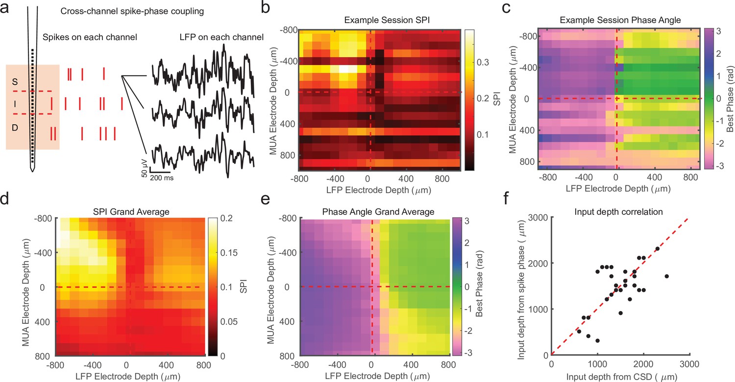
Cross-channel spike–local field potential (LFP) phase coupling reversal correlates with putative input layer.
(a) Schematic displaying cross-channel phase coupling analysis. The spike times on each channel are compared against the phase of the LFP on each other channel, yielding a matrix of spike-phase coupling. (b) Example recording session cross-channel spike-phase index (SPI) values from marmoset MT. Red dashed lines indicate the estimated depth of the bottom of the input layer from current-source density (CSD) analysis. (c) Preferred phase angles for the cross-channel spike-phase relationships in b. Spikes across all channels preferred ±π rad phase angles from LFP measure on superficial and input electrodes, but preferred 0 rad phase angles from LFP measured on deep phase angles. The LFP phase reversal aligns well to the estimate of the input layer from CSD analysis (red dashed line). (d) Grand average cross-channel SPI across all recording sessions in MT, V4, and PFC aligned to the putative input layer from CSD analysis (N = 34 sessions). (e) Grand average of the preferred phase angle for the data in d. (f) Scatter plot shows a significant correlation between the depth of the bottom of the input layer estimated from CSD analysis (x-axis) and the depth of the phase reversal (y-axis; Pearson’s r = 0.64, p = 0.00005).
Figure 3—figure supplement 1
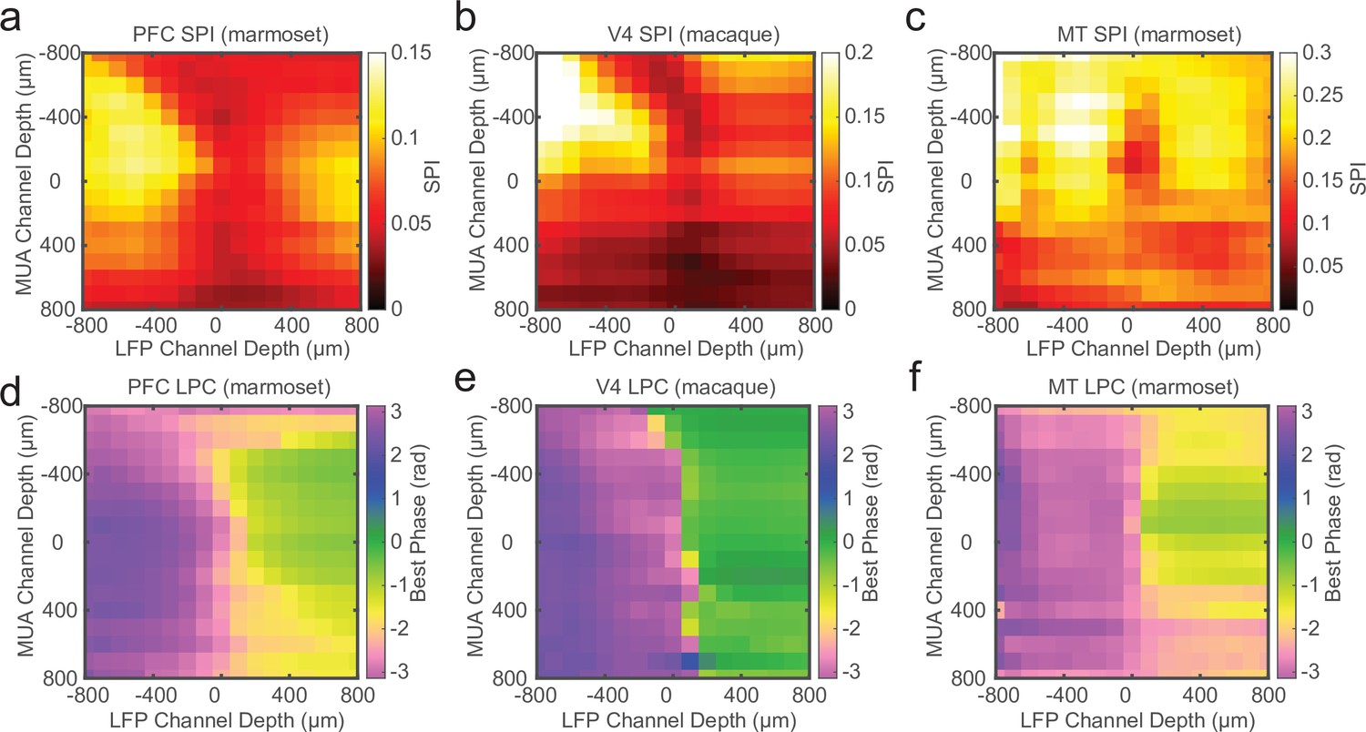
Laminar spike-phase reversal consistent across cortical areas.
Grand average cross-channel spike-phase index (SPI) measurements for sessions recorded in marmoset PFC (a; N = 14), macaque V4 (b; N = 12), and marmoset MT (c; N = 8). The depth measurements are relative to the estimate of the bottom of the input layer from current-source density (CSD) analysis. (d–f) Grand average cross-channel preferred spike-phase angles for the cortical areas as in a–c. The phase reversal is well aligned to the putative input layer estimated from CSD analysis.
Figure 3—figure supplement 2
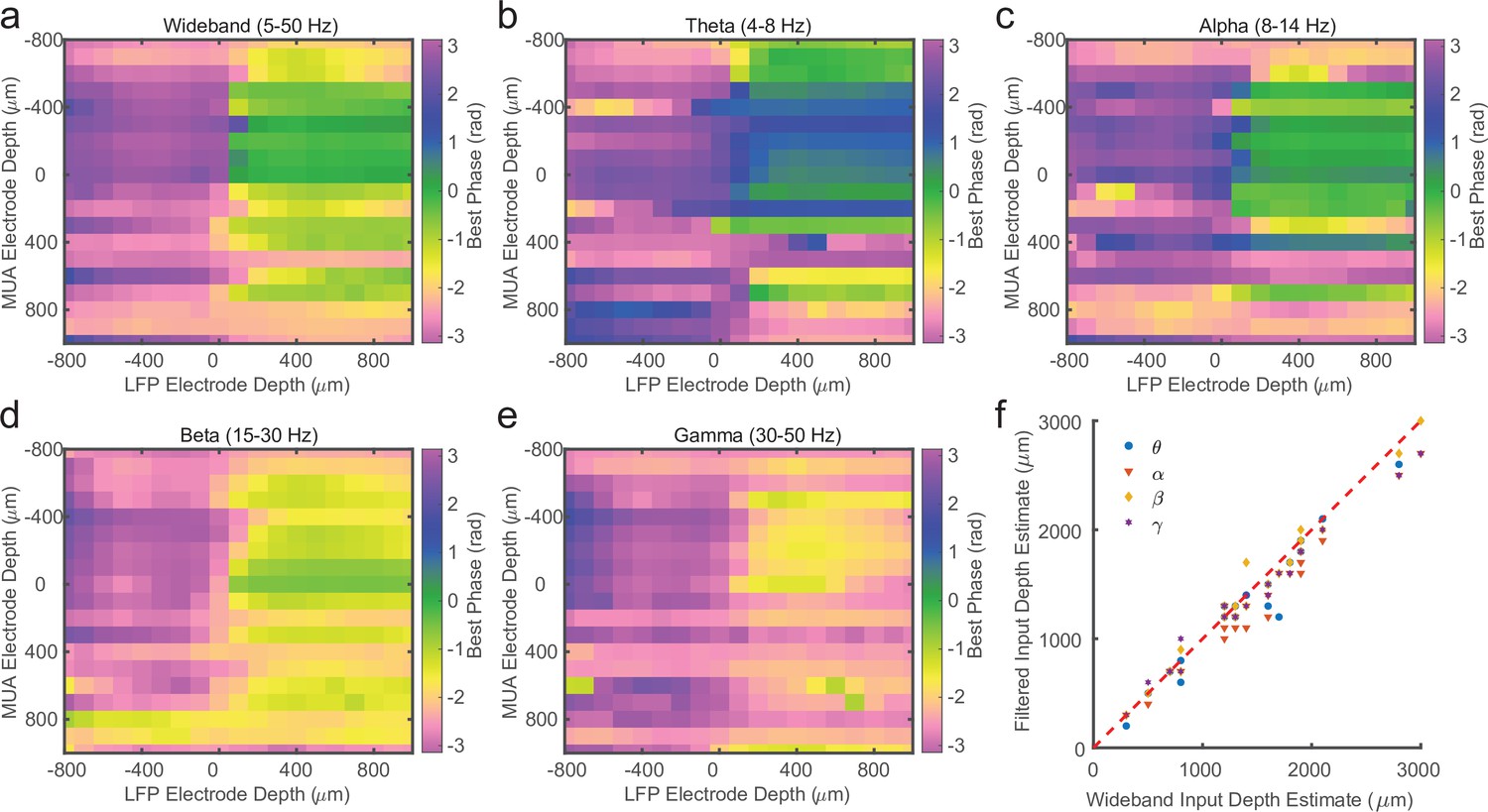
Laminar spike-phase pattern does not depend on filtering.
(a) Example cross-channel laminar-phase coupling (LPC) from marmoset MT after filtering local field potential (LFP) from 5 to 50 Hz calculated using Generalized Phase (GP). (b–e) Same as in a, but after filtering in theta (4–8 Hz), alpha (8–14 Hz), beta (15–30 Hz), or low gamma (30–50 Hz) frequency bands and measuring phase with the Hilbert Transform. The LPC reversal occurs at the same depth regardless of filter bandwidth. (f) Scatter plot showing the lack of dispersion from unity between depth estimates made using the 5–50 Hz filter or each of the tested narrowband filters.
Figure 3—figure supplement 3
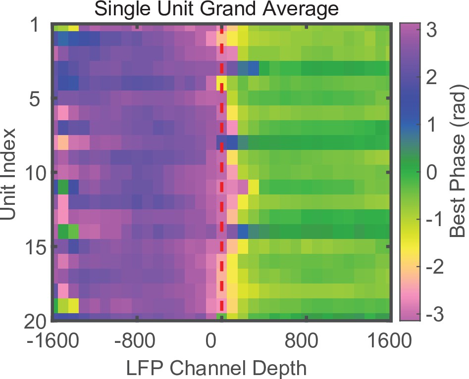
Phase reversal is apparent when using well-isolated single units instead of MUA.
Laminar-phase coupling (LPC) grand average across all sessions (N = 34) for well-isolated single units. Units were aligned across sessions relative to their index from the median index. The use of single-unit spiking instead of MUA produces qualitatively similar results.
Figure 3—figure supplement 4
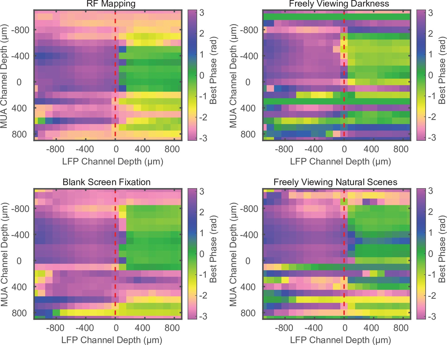
Phase relationship does not depend on task conditions.
Example cross-channel laminar-phase coupling (LPC) measurements for different experimental conditions during the same recording session. The spike-phase reversal is consistent across receptive field mapping, free viewing in total darkness, fixation on a blank screen during a visual detection task, or freely viewing naturalistic images. Example data from marmoset MT.
Figure 3—figure supplement 5
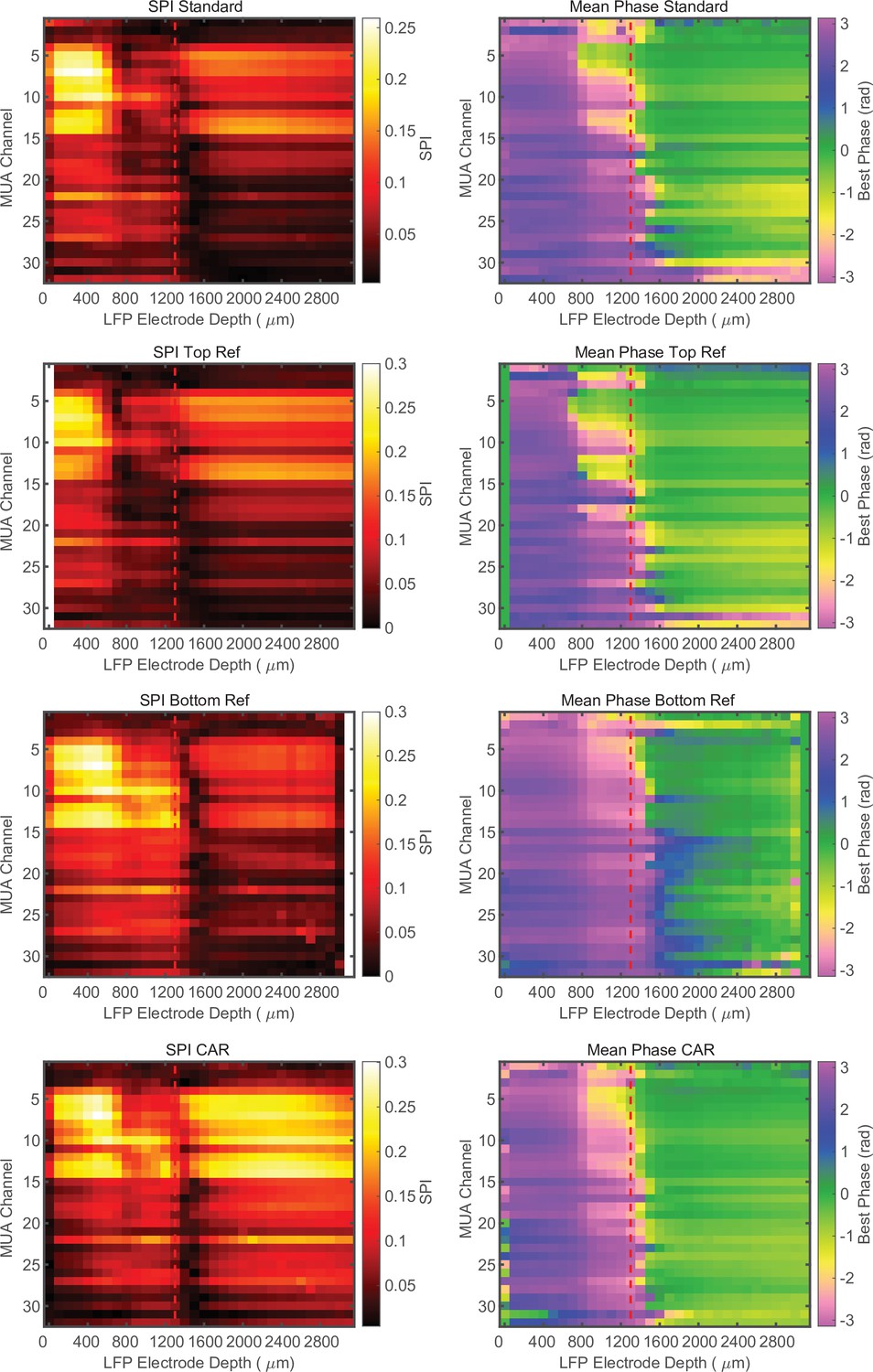
Phase relationship is not dependent on referencing.
Cross-channel laminar-phase coupling (LPC) measurements from the same recording session with the integrated reference contact, re-referencing to the top most contact, the bottom most contact, or a common average reference (CAR) from top to bottom, respectively. The presence of the laminar-phase reversal is not dependent on referencing. Example data from macaque V4.
Figure 3—figure supplement 6
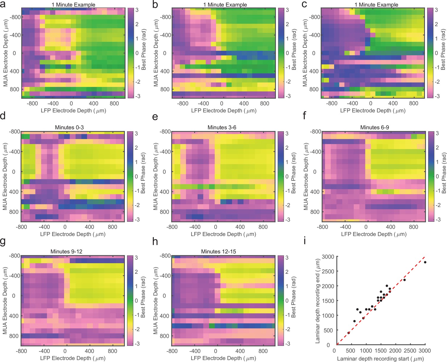
Cross-channel laminar-phase coupling (LPC) can be estimated over short periods.
(a–c) Cross-channel LPC measurements from three example sessions generated from 1 min of recorded data. The phase reversal in these sessions is well aligned to the estimate from the entire recording. (d) LPC measurement from the first 3 min of a different linear probe recording. (e–h) LPC measurements of the subsequent 3 min of the same recording in d. The location of the phase reversal drifts over the course of the first 15 min of the recording. (i) Scatter plot comparing the estimated depth of the phase reversal based on the first (x-axis) or last (y-axis) 2 min of the recording session (N = 19). Drift of 100–300 μm is consistently observed across recordings.
Figure 4
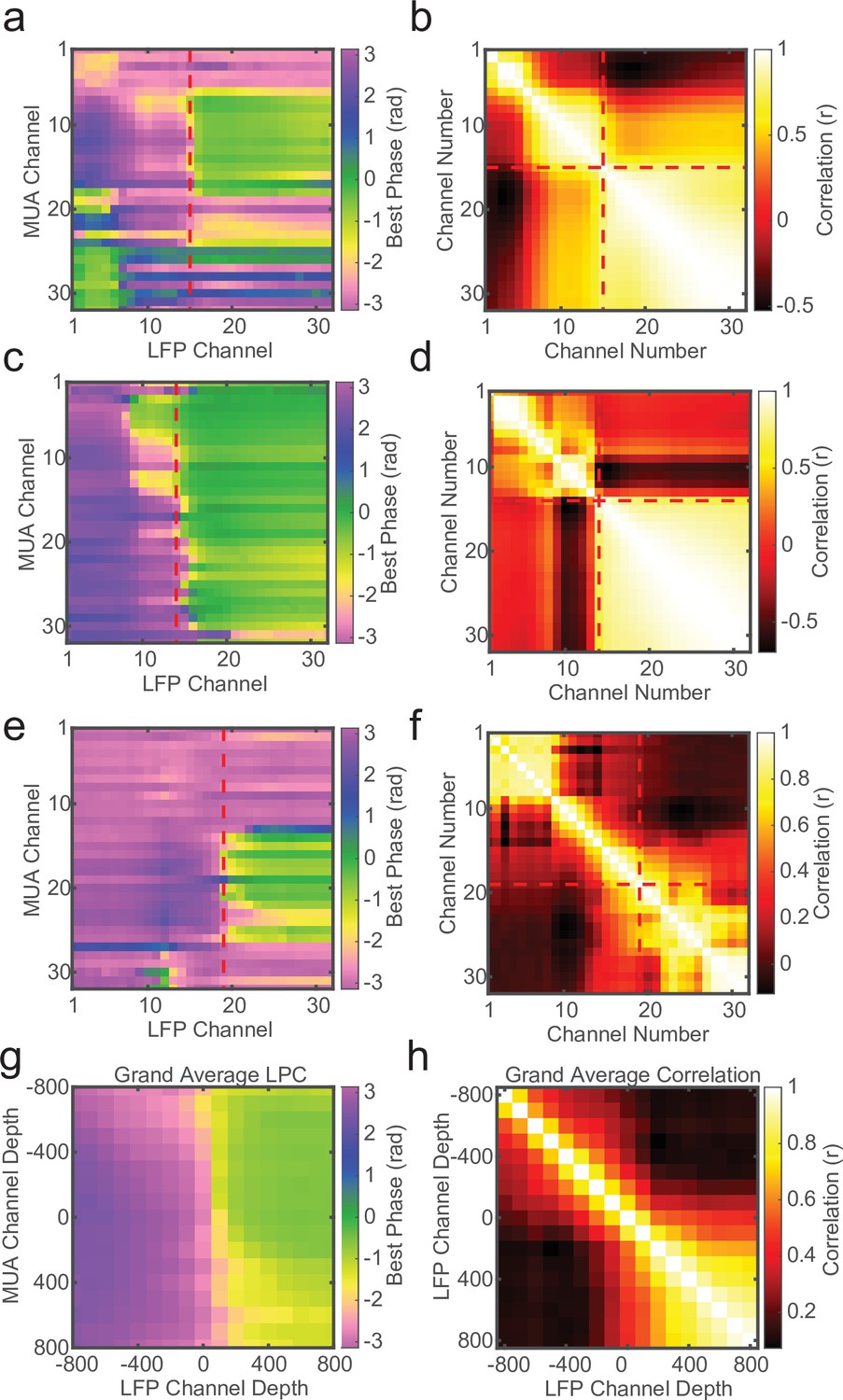
Local field potential (LFP)–LFP phase correlations can also reveal laminar boundaries, but are less consistent.
(a) Preferred phase angle across all 32 channels from an example marmoset recording. The red dashed line indicates the current-source density (CSD) estimate of the bottom of the input layer. (b) Circular LFP phase correlation across channels. There is a strong within compartment correlation that aligns with the boundary between channels above and below the input/deep boundary (red dashed lines). (c, d) Same as panels a and b, but for a macaque recording. (e, f) Same as above, but an example of poor phase correlation within compartments despite strong phase reversal alignment with CSD. (g, h) Grand averages for preferred phase angle and LFP phase correlations across all recording sessions (N = 34). Plots were aligned to the putative input/deep layer boundary identified by CSD analysis.
Figure 5
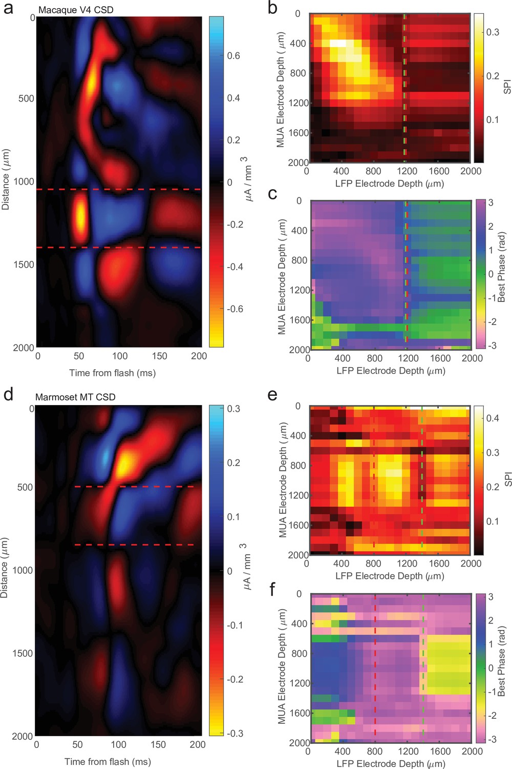
Current-source density (CSD) analysis is not always consistent with laminar-phase reversal.
(a) Example CSD from macaque V4 with estimate of input layer boundaries indicated by red dashed lines (N = 81 trials). (b) Cross-channel spike-phase index (SPI) for the same example recording as the CSD in a. Red line is the CSD estimate of the bottom of the input layer. Green line is the estimate from the phase reversal. (c) Cross-channel spike-phase pattern for same recording as in a and b. The phase reversal is well aligned to the CSD estimate of the input layer. (d) CSD from a different example recording session in marmoset MT (N = 661 trials). Laminar depth estimated the same as in a. (e, f) Cross-channel SPI and phase angle as in b and c. The CSD and phase reversal estimates do not align.
Figure 6
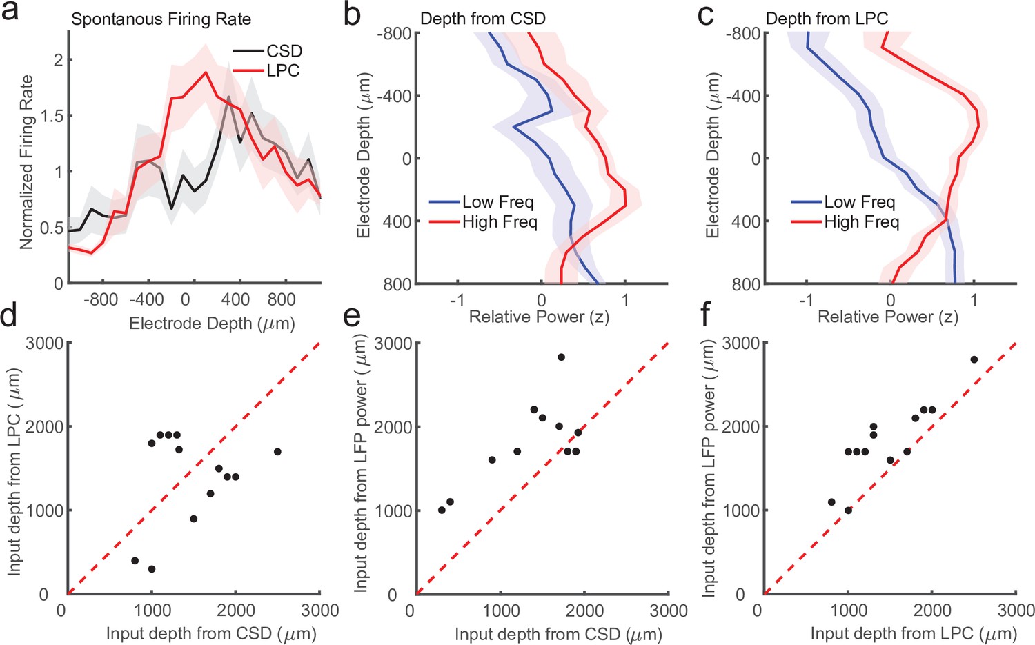
Laminar-phase coupling (LPC) pattern better replicates spike rate and local field potential (LFP) power dissociations than current-source density (CSD) when the two measures disagree.
(a) Normalized spontaneous firing rates across sessions when CSD and LPC disagreed as a function of contact depth by more than 200 μm (N = 14; shaded regions denote standard error of the mean [SEM]). LPC captures the expected higher spontaneous firing rates around the input layer. (b) Mean z-scored LFP power across sessions in lower frequencies (8–30 Hz, blue line) and higher frequencies (65–100 Hz, red line) as a function of electrode depth referenced to the CSD estimate for sessions. (c) Same as in a, but referenced to the depth estimate from the LPC phase reversal across sessions. The laminar power relationship is more pronounced when using the phase reversal instead of CSD estimate. (d) Scatter plot showing the disagreement in the depth of the input layer estimated from CSD (x-axis) and the depth from LPC (y-axis) in this subset of recording sessions. (e) Scatter plot showing the alignment of the CSD input depth (x-axis) crossover in LFP power (y-axis). (f) Same as e, but for LPC. The LPC depth measure was more correlated with the LFP power reversal than the CSD measure (Pearson’s r = 0.65 vs. 0.87 CSD vs. LPC).
Additional files
Download links
A two-part list of links to download the article, or parts of the article, in various formats.
Downloads (link to download the article as PDF)
Open citations (links to open the citations from this article in various online reference manager services)
Cite this article (links to download the citations from this article in formats compatible with various reference manager tools)
Spike-phase coupling patterns reveal laminar identity in primate cortex
eLife 12:e84512.
https://doi.org/10.7554/eLife.84512


