A stable, distributed code for cue value in mouse cortex during reward learning
- Center for the Neurobiology of Addiction, Pain and Emotion, University of Washington, United States
- Anesthesiology and Pain Medicine, University of Washington, United States
- Department of Biological Structure, University of Washington, United States
- Department of Pharmacology, University of Washington, United States
Figures
Figure 1 with 2 supplements
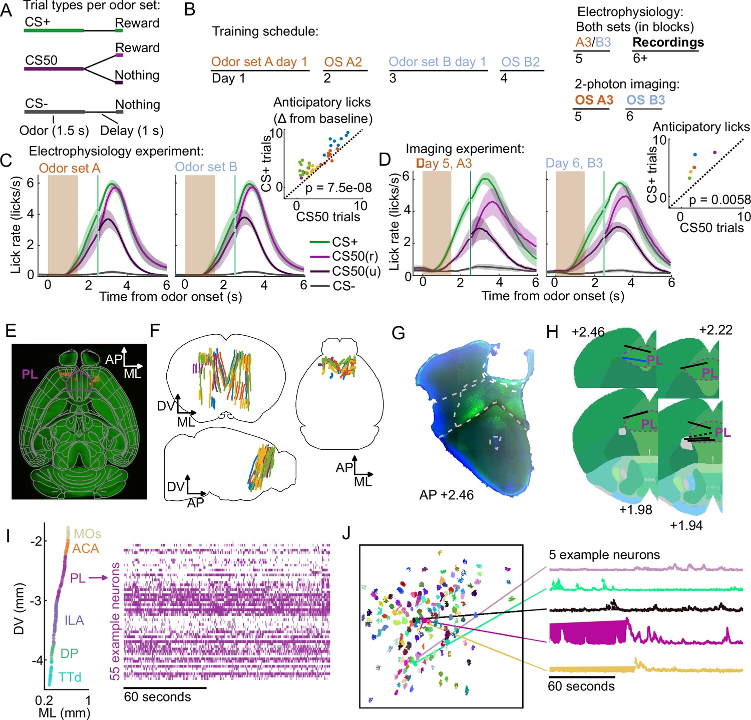
Electrophysiology and calcium imaging during olfactory Pavlovian conditioning.
(A) Trial structure in Pavlovian conditioning task. (B) Timeline for mouse training. (C) Mean (+/− standard error of the mean (SEM)) lick rate across mice () on each trial type for each odor set during electrophysiology sessions. CS50(r) and CS50(u) are rewarded and unrewarded trials, respectively. Inset: mean anticipatory licks (change from baseline) for the CS+ and CS50 cues for every session, color-coded by mouse. for a main effect of cue in a two-way ANOVA including an effect of subject. (D) Same as (C ), for the third session of each odor set ( mice). for a t-test comparing anticipatory licks on CS+ and CS50 trials. (E) Neuropixels probe tracks labeled with fluorescent dye (red) in cleared brain (autofluorescence, green). AP, anterior/posterior; ML, medial/lateral; DV, dorsal/ventral. Allen common-coordinate framework (CCF) regions delineated in gray. Outline of prelimbic area in purple (F) Reconstructed recording sites from all tracked probe insertions ( insertions, mice), colored by mouse. (G) Sample histology image of lens placement. Visualization includes DAPI (blue) and GCaMP (green) signal with lines indicating cortical regions from Allen Mouse Brain Common Coordinate Framework. (H) Location of all lenses from experimental animals registered to Allen Mouse Brain Common Coordinate Framework. Blue line indicates location of lens in (A). The dotted black line represents approximate location of tissue that was too damaged to reconstruct an accurate lens track. The white dotted line indicates prelimbic area (PL) borders.(I) ML and DV coordinates of all neurons recorded in one example session, colored by region, and spike raster from example PL neurons. (J) ROI masks for identified neurons and fluorescence traces from five example neurons.
Figure 1—figure supplement 1
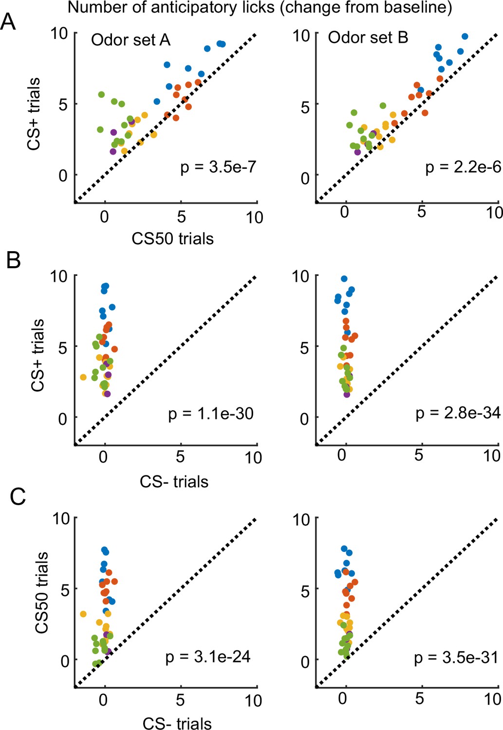
Anticipatory licking during the electrophysiology sessions.
(A) Mean anticipatory licks (change from baseline) for the CS+ and CS50 from odor set A (left) and B (right) for every session, color-coded by mouse. and in each odor set for a main effect of cue in a two-way ANOVA including an effect of subject. (B) As above, for the CS+ and CS− from odor set A (left) and B (right). and in each odor set for a main effect of cue in a two-way ANOVA including an effect of subject. (C) As above, for the CS50 and CS− from odor set A (left) and B (right). and in each odor set for a main effect of cue in a two-way ANOVA including an effect of subject.
Figure 1—figure supplement 2
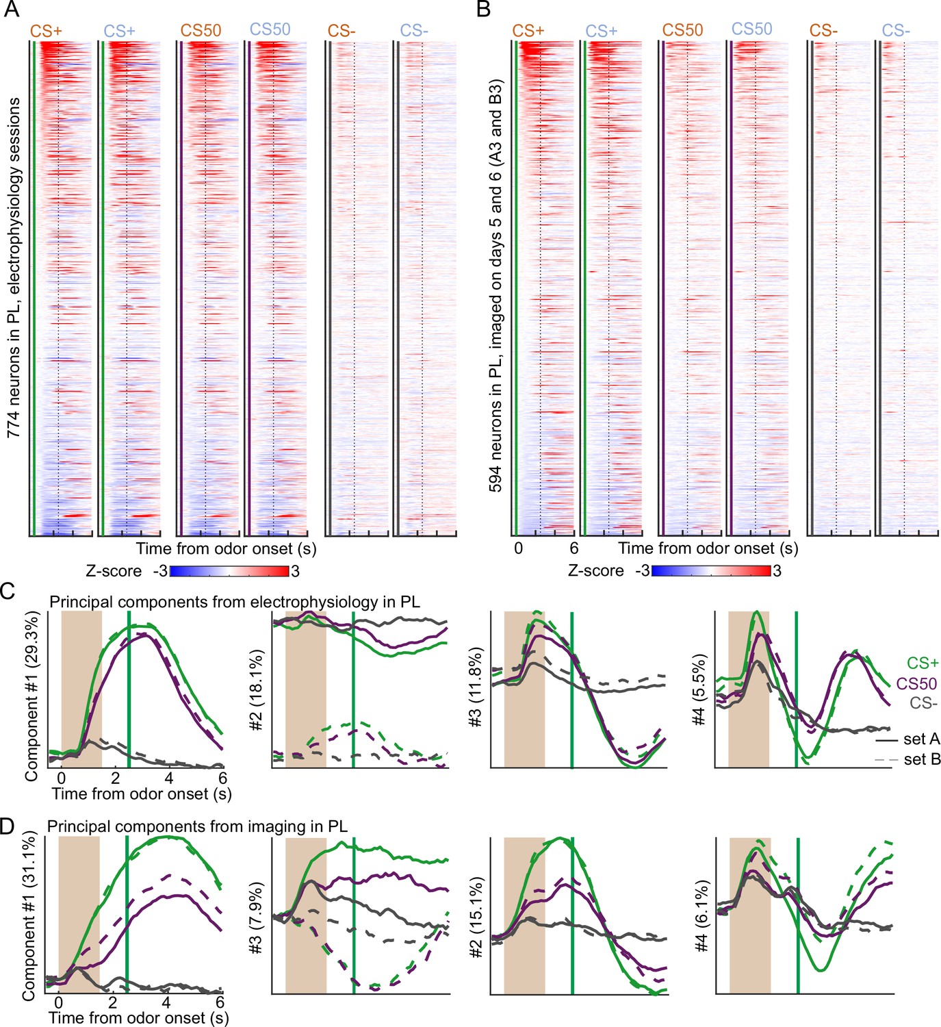
Similar neural activity in prelimbic area using electrophysiology and calcium imaging.
(A) Heatmap of the normalized activity of each neuron recorded with electrophysiology in prelimbic area (PL), aligned to each of the six odors. All columns sorted by mean firing 0 - 1.5s following odor onset for odor set A CS+ trials. (B) As in (A), for all neurons imaged in PL on day 3 of each odor set. (C) The score from the first four principal components of the normalized activity presented in (A), with variance explained in parentheses. (D) As in (C), for the activity in (B).
Figure 2 with 4 supplements
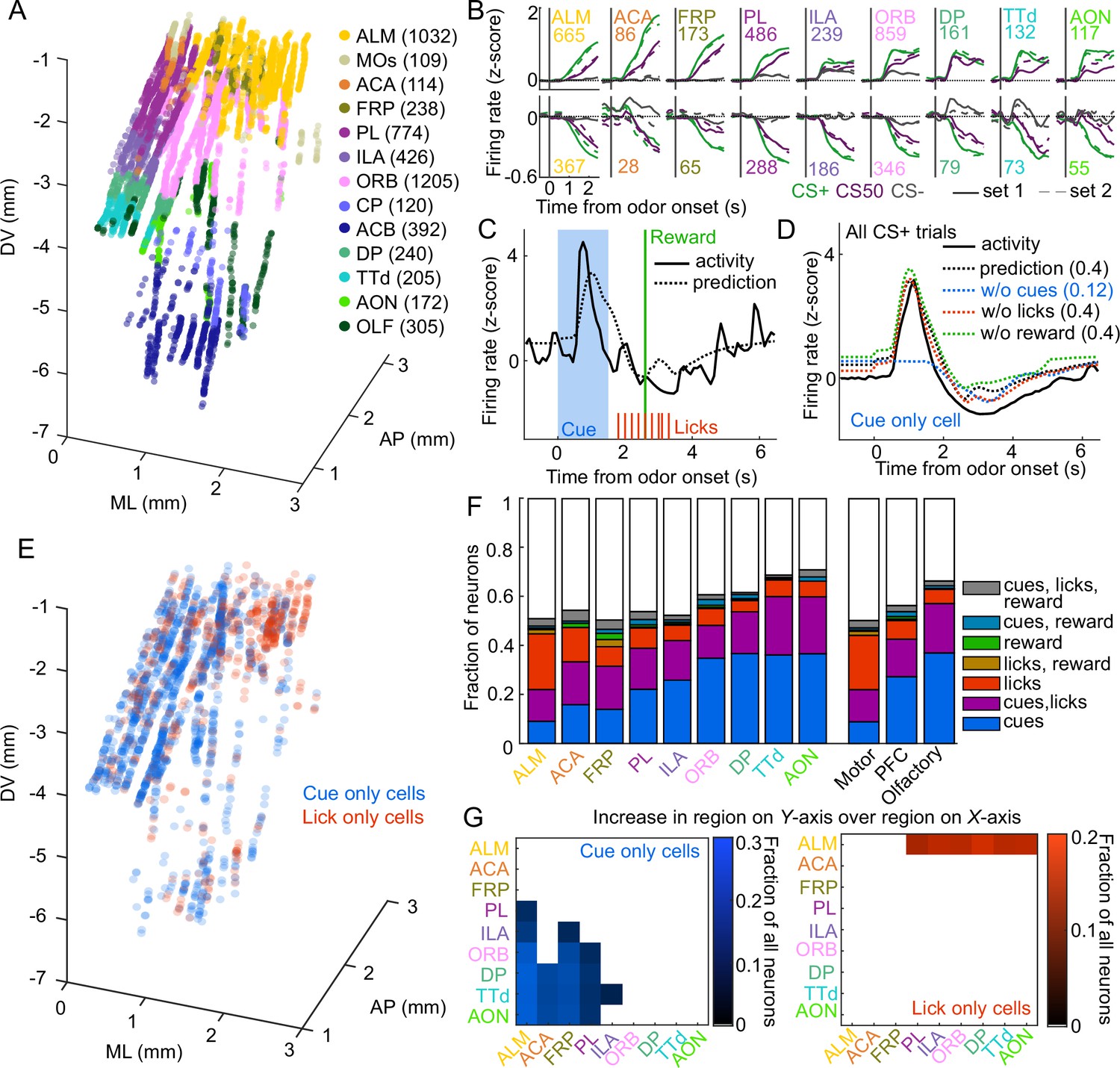
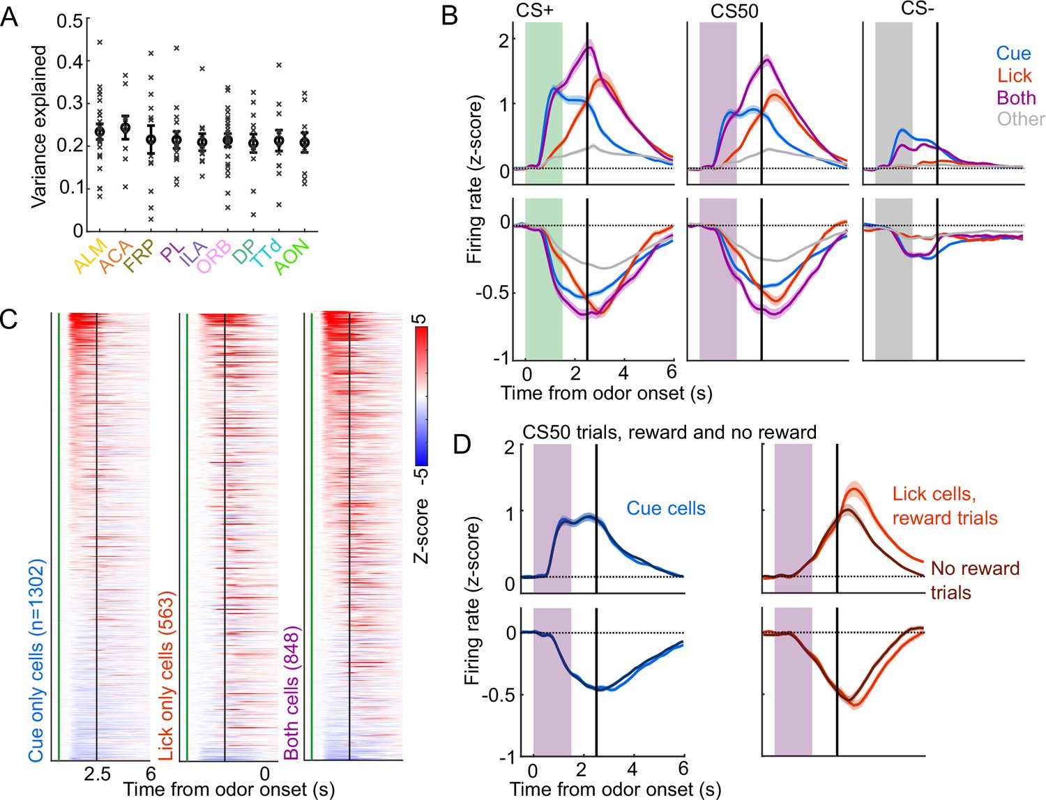
Graded cue and lick coding across the recorded regions.
(A) Location of each recorded neuron relative to bregma, projected onto one hemisphere. Each neuron is colored by common-coordinate framework (CCF) region. Numbers indicate total neurons passing quality control from each region. (B) Mean normalized activity of all neurons from each region, aligned to odor onset, grouped by whether peak cue activity (0–2.5 s) was above (top) or below (bottom) baseline in held out trials. Number of neurons noted for each plot. (C) Example kernel regression prediction of an individual neuron’s normalized activity on an example trial. (D) CS+ trial activity from an example neuron and predictions with full model and with cues, licks, and reward removed. Numbers in parentheses are model performance (fraction of variance explained). (E) Coordinates relative to bregma of every neuron encoding only cues or only licks, projected onto one hemisphere. (F) Fraction of neurons in each region and region group classified as coding cues, licks, reward, or all combinations of the three. (G) Additional cue (left) or lick (right) neurons in region on Y-axis compared to region on x-axis as a fraction of all neurons, for regions with statistically different proportions (see Methods).
Figure 2—figure supplement 1

Task-related neural activity across brain regions.
(A) For each of the 5 mice in the electrophysiology experiment, the number of neurons recorded in each region. (B) Heatmap of the normalized activity of each neuron ( trials per cue). All columns sorted by region and then by mean firing 0–1.5s following odor onset for odor set A CS+ trials. (C) Mean (+/− SEM) activity of neurons from four regions aligned to each cue type, grouped by whether peak cue activity (0–2.5 s) was above (top) or below (bottom) baseline in held out trials.
Figure 2—figure supplement 2
Identification of cue and lick cells with GLM.
(A) Mean variance explained (fraction) by linear models in each region for each session (x) and the mean (+/− SEM) across those sessions. (B) Mean (+/− SEM) activity of neurons encoding cues, licks, both, or neither aligned to each cue type, grouped by whether peak cue activity (0–2.5s) was above (top) or below (bottom) baseline in held out trials. (C) Normalized activity of every neuron encoding cues, licks, or both, aligned to CS+ onset, sorted by mean firing 0–1.5s following odor onset. (D) Mean (+/− SEM) activity of neurons encoding cues or licks, grouped as in (B), on CS50 trials, divided into rewarded (lighter colors) or unrewarded (darker colors) trials.
Figure 2—figure supplement 3
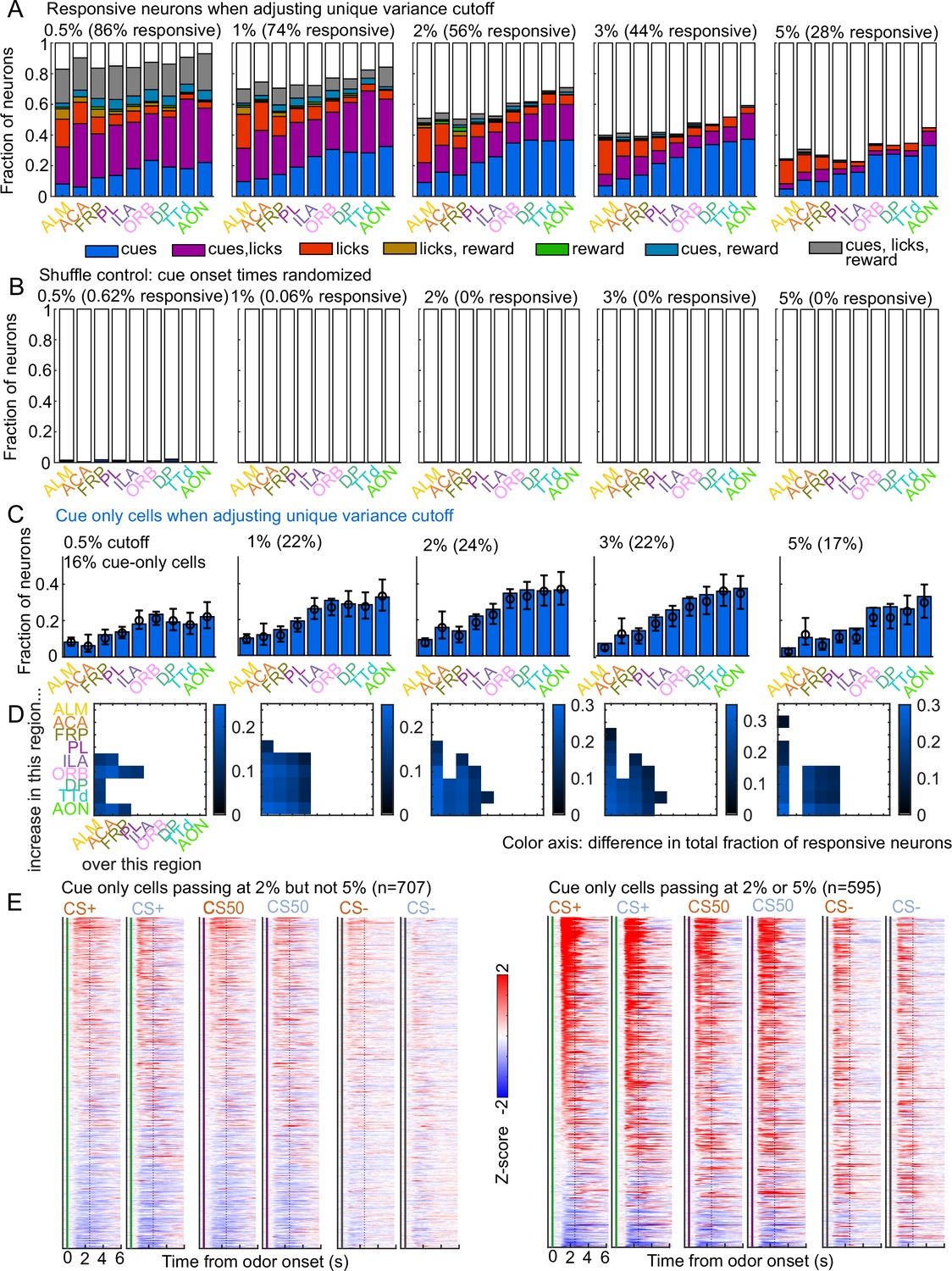
Validation of variance cutoff for variable coding.
(A) Fraction of neurons encoding cues, licks, and rewards in each region when varying the unique variance cutoff used (how much model performance drops when removing that variable). (B) As in (A), for models where the reduced ranks are fit to neural activity with shuffled cue onset times. (C) The fraction of cue cells (neurons with unique cue variance but no other variables) in each region when varying the variance cutoff. (D) Pairwise region comparisons with each variance cutoff. (E) Normalized activity of every neuron encoding cues, sorted by mean firing 0 - 1.5s following odor onset. Left: neurons only passing as cue only with a 2% cutoff but a 5% cutoff. Right: neurons passing as cue only with either a 2% or a 5% cutoff.
Figure 2—figure supplement 4

Comparing proportions of cue and lick neurons across regions.
(A) Fraction of neurons in each region classified as coding cues (left), licks (middle), or both (right), as well as estimated fraction(± 95% CI) with random effect of session (see Methods). Data also shown in Figure 2F. (B) Additional cue/lick/both cells in region on y-axis compared to region on x-axis as a fraction of all neurons, for regions with significantly different proportions. Pairwise comparisons in Supplementary file 1. Data also shown in Figure 2G. (C) As in (A), for region groups. (D) As in (B), for region groups.
Figure 3 with 2 supplements
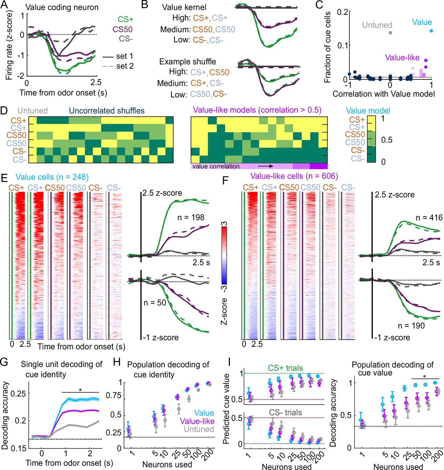
Robust value encoding and decoding among cue cells.
(A) Normalized activity of an example value cell with increasing modulation for cues with higher reward probability.(B) For the same neuron, model-fit cue kernel for the original value model and with one of the 152 alternatively-permuted cue coding models. (C) Distribution of best model fits across all cue neurons. Light blue is value model, purple is value-like models, gray is untuned model, and the remaining models are dark blue. Value-like models are shaded according to their correlation with ranked value, as illustrated in (D). Dashed line is chance proportion when assuming even distribution. (D) Schematic of value assigned to each of the six cues for many of the cue coding models (full schematic in Figure 3—figure supplement 1). Value-like models are sorted by their correlation with the ranked value model. (E) Left: normalized activity of every value cell, sorted by mean firing 0–1.5s following odor set A CS+ onset. Right: mean normalized activity of all value cells, grouped by whether peak cue activity (0–2.5s) was above (top) or below (bottom) baseline in held out trials. Number of neurons noted for each plot. (F) As in (E), for value-like cells. (G) Accuracy (mean ± SEM across neurons) of decoded cue identity for single neurons of value (), value-like (), and untuned () neurons. * indicates where value, value-like, and untuned neurons significantly differed from each other and baseline (all , Bonferroni corrected). All pairwise comparisons in Supplementary file 2. (H) Accuracy (mean ± SD across bootstrapped iterations) of decoded cue identity using different numbers of neurons. (I) Left: estimated value (mean ± SD across 1000 bootstrapped iterations) of held out CS+ (top) and CS− (bottom) trials using linear models trained on the activity of value, value-like, or untuned neurons. Right: accuracy (mean ± SD across bootstrapped iterations) of decoded cue value using these value estimates. * indicates where the accuracy of value neurons exceeded value-like and untuned neurons (all , bootstrapped). All pairwise comparisons in Supplementary file 2.
Figure 3—figure supplement 1

Schematic of value model shuffles.
(A) For each of the 153 cue coding models, the value taken on by the variable cue kernel on trials corresponding to each of the six cue types. Values were 0, 0.5, or 1. Also, the fraction of cue neurons best fit by each model. Dashed line is chance proportion when assuming even distribution. (B) As in (A), sorted by correlation with the ranked value model. (C) Data from Figure 3C with color indicating models with the same values for cues of the same trial type across odor sets. Dashed line is chance proportion when assuming even distribution.
Figure 3—figure supplement 2

Population analysis of value coding schemes.
(A) Projecting the activity (0 to 2.5s from odor onset) of all value and value-like cells onto the coding dimensions maximally separating CS− and CS+ (x-axis) and CS− and CS50 (y-axis). X marks baseline activity. (B) For the odor set A projection, distribution of 5000 bootstrapped angles between CS+ and CS50 vectors (baseline to peak). Value cells had a smaller angle than value-like cells, evidence of a linear value scale.
Figure 4 with 3 supplements
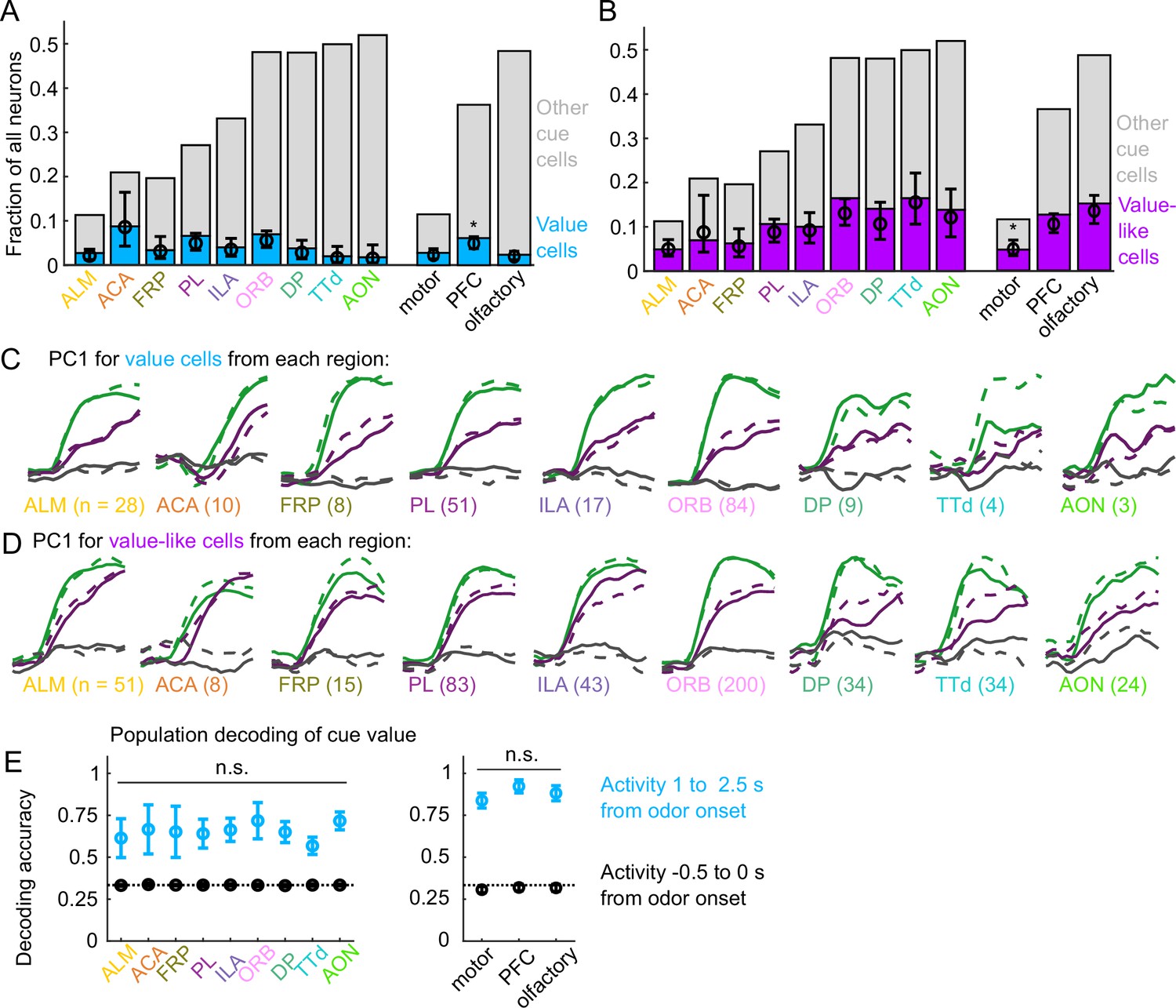
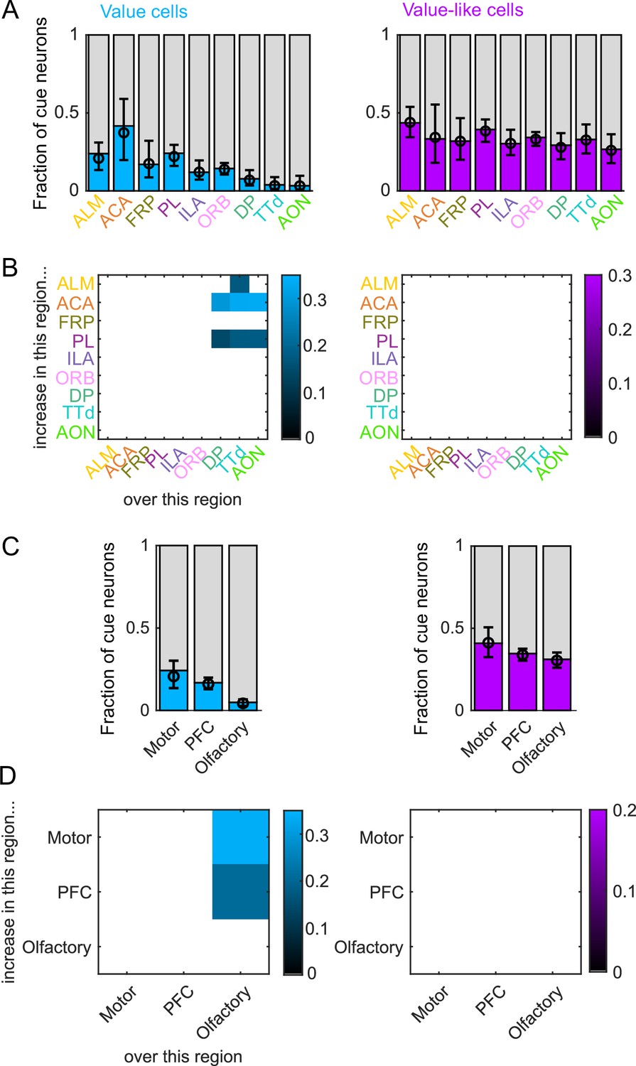
Widespread cue value coding.
(A) Fraction of neurons in each region and region group classified as value cells (blue) and other cue neurons (gray), as well as fraction (± 95% CI) estimated from a linear mixed effects model with random effect of session (see Methods). Prefrontal cortex (PFC) has more value cells than motor () and olfactory () cortex. All pairwise comparisons in Supplementary file 3. (B) As in (A), for value-like cells. Motor cortex has fewer value-like cells than PFC () and olfactory cortex (). All pairwise comparisons in Supplementary file 3. (C) First principal component value cells from all regions. (D) As in (C), for value-like cells. (E) Accuracy of decoded cue value (mean ± SD across 1000 bootstrapped iterations) as in Figure 3I, using five (with replacement) value cells from each region (left) and 25 value cells from each region group (right) using cue-evoked (blue) and baseline (black) activity. No regions or region groups significantly differed from each other (, Bonferroni corrected). All pairwise comparisons in Supplementary file 3.
Figure 4—figure supplement 1

Relative proportions of value and value-like cells across regions.
(A) Additional cue value (left) or value-like (right) neurons in region on y-axis compared to region on x-axis as a fraction of all neurons, for regions with non-overlapping 95% confidence intervals. (B) As in (A), for region groups.
Figure 4—figure supplement 2
Value coding as a proportion of cue cells.
(A) Fraction of cue neurons in each region classified as coding value (left) or value-like (right), as well as estimated fraction(± 95% CI) with random effect of session (see Methods). (B) Additional value/value-like cue neurons in region on y-axis compared to region on x-axis as a fraction of all cue neurons, for regions with significantly different fractions. Pairwise comparisons in Supplementary file 5. (C) As in (A), for region groups. (D) As in (B), for region groups.
Figure 4—figure supplement 3
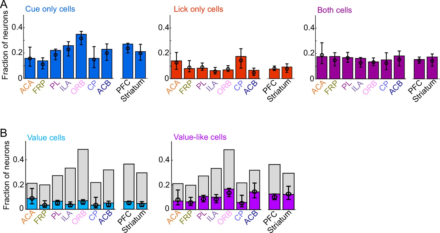
Comparing prefrontal cortex (PFC) and striatum.
(A) Fraction of neurons in each region and region group classified as coding cues (left), licks (middle), or both (right), as well as estimated fraction(± 95% CI) with random effect of session (see Methods). (B) Fraction of neurons in each region and region group classified as coding value (left) or value-like (right), as well as estimated fraction(± 95% CI) with random effect of session. Light gray bars are remaining cue neurons not in that category.
Figure 5
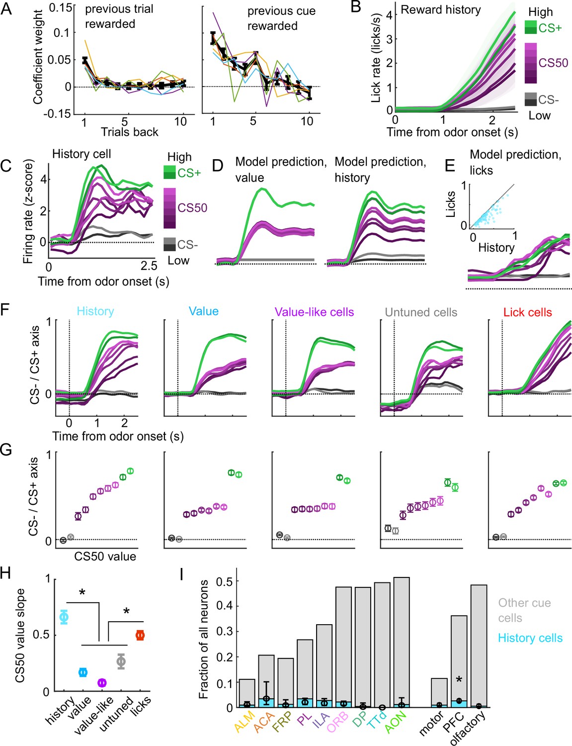
A subset of cue cells incorporate reward history.
(A) Coefficient weight (± standard error from model fit) for reward outcome on the previous 10 trials of any type (left) and on the previous 10 trials of the same cue type (right) for the ‘trial value’ model: a linear model predicting the number of anticipatory licks on every trial of every session. Lick rates were normalized so that the maximum lick rate for each session was equal to 1. Colored lines are models fit to each individual mouse. (B) Mean (± SEM) lick rate across mice ( mice) on trials binned according to value estimated from the trial value model. (C) Normalized activity of an example history value cell with increasing modulation for cues of higher value. (D) For the same neuron, model-predicted activity with the original value model (left) and with the history model, which uses trial-by-trial value estimates from the trial value model (right). (E) For the same neuron, model-predicted activity using licks. Inset: variance explained using licks versus history for history neurons. (F) The activity of all cells in each category projected onto the coding dimension maximally separating CS− and CS+ for trials binned by value estimated from the trial value model. (G) The mean (± SD across 5000 bootstrapped selections of neurons) activity (1–2.5s from odor onset) along the coding dimension maximally separating CS− and CS+ for trials binned by value estimated from the lick model. (H) The mean (± SD across 5000 bootstrapped selections of neurons) slope of the activity on CS50 trials regressed onto the trial value model estimate for those trials. History and lick cells had greater slopes than the other groups (, see Supplementary file 4). (I) Fraction of neurons in each region and region group classified as history cells (light blue) and other cue neurons (gray), as well as estimated fraction (± 95% CI) with random effect of session (see Methods). Prefrontal cortex (PFC) had more history cells than motor () and olfactory () cortex. All pairwise comparisons in Supplementary file 4.
Figure 6
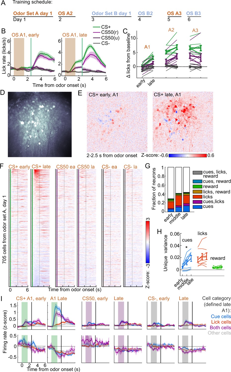
Acquisition of conditioned behavior and cue encoding in prefrontal cortex (PFC).
(A) Training schedule for five of the mice in the calcium imaging experiment. An additional three were trained only on odor set A. (B) Mean (± SEM) licking on early (first 60) and late (last 60) trials from day 1 of odor set A ( mice). (C) Mean (± SEM) baseline-subtracted anticipatory licks for early and late trials from each day of odor set A. Thin lines are individual mice ( mice). (D) Standard deviation of fluorescence from example imaging plane. (E) Normalized activity of each pixel following CS+ presentation on early and late trials of session A1. (F) Normalized deconvolved spike rate of all individual neurons on early and late trials of session A1. (G) Proportion of neurons classified as coding cues, licks, rewards, and all combinations for each third of session A1. (H) Mean(± SEM across mice) unique variance explained by cues, licks, and rewards for neurons from each mouse. Thin lines are individual mice. Unique variance was significantly different across session thirds for cues (, ) but not licks (, ) or reward (, , mice, one-way ANOVA). (I) Mean (± SEM) normalized deconvolved spike rate for cells coding cues ( above, below), licks ( above, below), both ( above, below), or neither ( above, below) on early and late trials, sorted by whether peak cue activity (0–2.5 s) was above (top) or below (bottom) baseline for late trials.
Figure 7 with 1 supplement
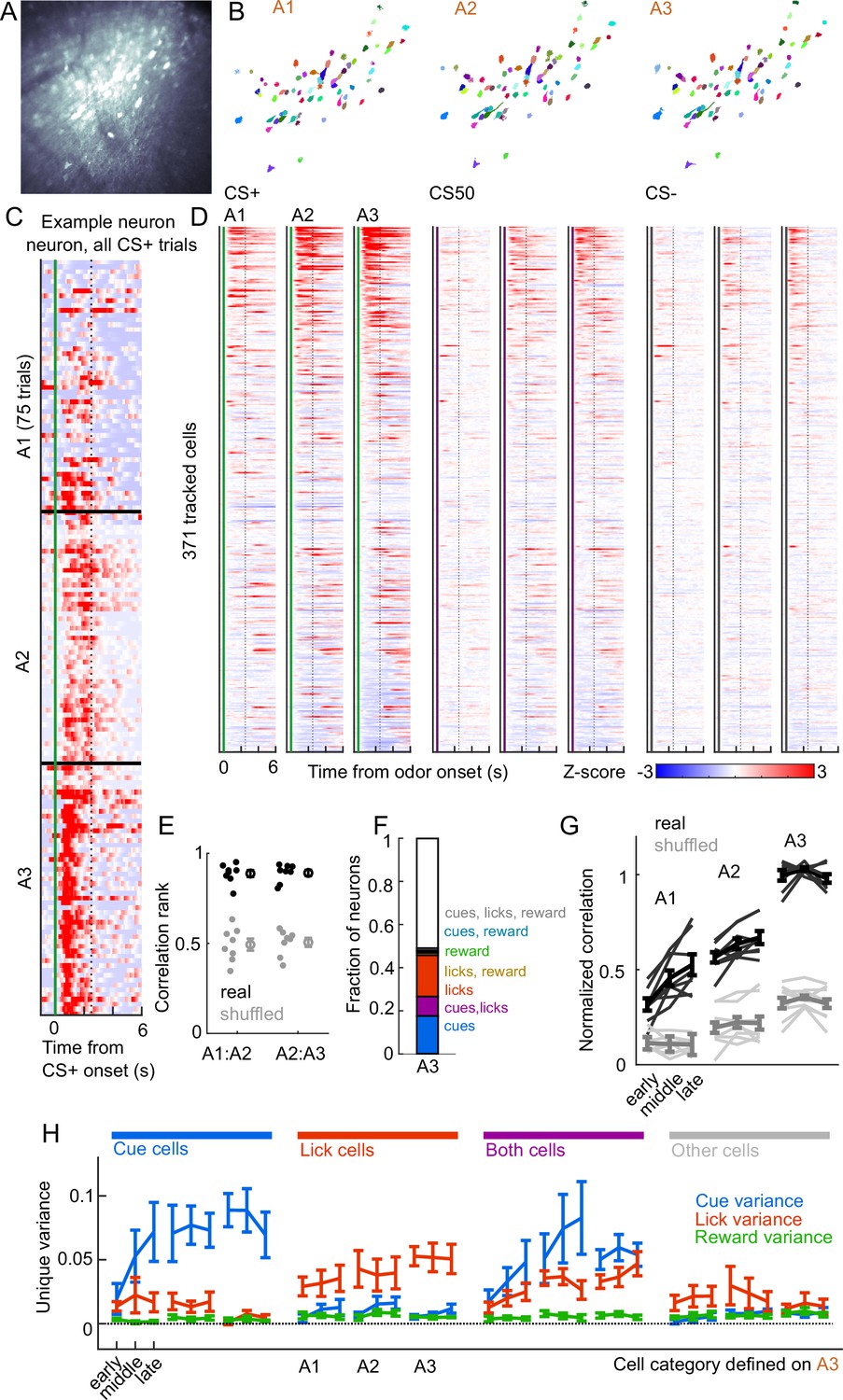
Cue and lick coding is stable across days.
(A) Standard deviation fluorescence from example imaging plane. (B) Masks (randomly colored) for all tracked neurons from this imaging plane. (C) Deconvolved spike rate on every CS+ trial from all three sessions of odor set A for an example neuron. Vertical dashed line is reward delivery. Color axis as in (D). (D) Normalized deconvolved spike rate for all tracked neurons on all three sessions of odor set A. (E) Correlation between the activity of a given neuron in one session and its own activity in the subsequent session, quantified as a percentile out of correlations with the activity of all other neurons on the subsequent day. Plotted as the median for each subject and the mean (± SEM) across these values. Real data was more correlated than shuffled data ( for both comparisons, Wilcoxon signed-rank test). (F) Fraction of tracked neurons coding cues, licks, rewards, and their combinations on day 3. (G) Model performance when using models from session A3 to predict the activity of individual neurons across session thirds of odor set A training, plotted as mean (± SEM) correlation between true and predicted activity across mice, normalized to the correlation between model and training data. Thin lines are individual mice. Performance was greater than shuffled data at all time points (, Bonferroni-corrected, mice). Non-normalized data in Figure 7—figure supplement 1. (H) Mean (± SEM across mice) unique cue, lick, and reward variance for cells classified as coding cues, licks, both, or neither on session A3. A3 cue cells had increased cue variance in A2 (, see Methods) and A1 () relative to lick and reward variance. Same pattern for A3 lick cells in A2 () and A1 ().
Figure 7—figure supplement 1

Correlation across days in prelimbic area (PL).
(A) Cumulative distribution of percentile of correlation for the activity of a given neuron with its own activity on the subsequent day compared to its correlation with the activity of all other neurons. True data (black) and shuffled data (gray), revealing strong enrichment of correlated activity for a tracked neuron across days. (B) Model performance when using models from session A3 to predict the activity of individual neurons across session thirds of odor set A training, plotted as mean (± SEM) correlation between true and predicted activity across mice. Thin lines are individual mice. Performance was greater than shuffled data at all time points () except early day 1 (, Bonferroni-corrected, mice).
Figure 8
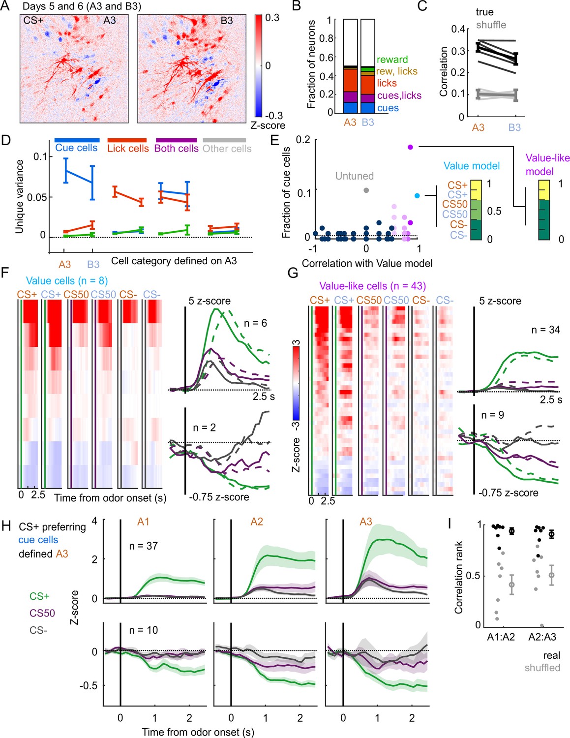
Stable cue coding across separately trained odor sets.
(A) Normalized activity of all pixels in the imaging plane following CS+ presentation on the third day of each odor set (A3 and B3, days 5 and 6 of training). (B) Fraction of neurons coding for cues, licks, rewards, and their combinations in A3 and B3 (days 5 and 6). (C) Mean (± SEM, across mice) correlation between activity predicted by odor set A3 models and its training data (A3, cross-validated) or activity in B3, for true (black) and trial shuffled (gray) activity. Thin lines are individual mice. , for main effect of odor set, , for main effect of shuffle, , for interaction, mice, two-way ANOVA. (D) Mean (± SEM, across mice) unique cue, lick, and reward variance for cells classified as coding cues, licks, both, or neither for odor set A. For each category, odor set A unique variance preference was maintained for odor set B () except for both cells, for which lick and reward variance were not different in odor set B (, Bonferroni-corrected, mice). (E) Distribution of best model fits across all cue cells, with colors from Figure 3C. Dashed line is chance proportion when assuming even distribution. (F) Left: normalized activity of every value cell, sorted by mean firing 0–1.5s following odor set A CS+ onset. Right: mean normalized activity of all value cells, grouped by whether peak cue activity (0–2.5 s) was above (top) or below (bottom) baseline in held out trials. Number of neurons noted for each plot. (G) As in (E), for value-like cells. (H) Mean (± SEM, across neurons) activity of cue cells tracked across A1, A2, and A3 with preferential CS+ firing, defined on half of A3 trials and plotted for the other half of A3 trials and all of A1 and A2 trials. (I) For neurons in (H), correlation between a neuron’s activity in one session and its own activity in the subsequent session, quantified as a percentile out of correlations with the activity of all other neurons on the subsequent day. Plotted as the median for each subject ( with CS+ preferring cue cells) and the mean (± SEM) across these values. Real data was more correlated than shuffled data ( A1:A2, A2:A3, Wilcoxon signed-rank test).
Additional files
-
Supplementary file 1
Statistics related to Figure 2G and Figure 2—figure supplement 4.
Bonferroni-corrected p-values from region contrast in generalized linear mixed-effects model.
- https://cdn.elifesciences.org/articles/84604/elife-84604-supp1-v1.docx
-
Supplementary file 2
Statistics related to Figure 3.
Top: Bonferroni-corrected p-values from pairwise comparisons between the decoding accuracy of each group of neurons at each time point with their performance at baseline and with the other neuron groups at that time point. Middle, Bottom: Bonferroni-corrected p-values for pairwise comparisons of bootstrapped distributions (1000 samples) of decoding performance using increasing numbers of neurons in each group.
- https://cdn.elifesciences.org/articles/84604/elife-84604-supp2-v1.docx
-
Supplementary file 3
Statistics related to Figure 4.
Top, Middle: Bonferroni-corrected p-values from region contrasts in generalized linear mixed-effects model. Bottom: Bonferroni-corrected p-values for pairwise comparisons of bootstrapped distributions (1000 samples) of decoding performance using value cells from each region.
- https://cdn.elifesciences.org/articles/84604/elife-84604-supp3-v1.docx
-
Supplementary file 4
Statistics related to Figure 5.
Top: Bonferroni-corrected p-values for pairwise comparisons of bootstrapped distributions (5000 samples) of the slope of population activity of each group of neurons across CS50 trials of increasing value. Bottom: Bonferroni-corrected p-values from region contrasts in generalized linear mixed-effects model.
- https://cdn.elifesciences.org/articles/84604/elife-84604-supp4-v1.docx
-
Supplementary file 5
Statistics related to Figure 2G and Figure 2—figure supplement 4.
Bonferroni-corrected p-values from region contrast in generalized linear mixed-effects model.
- https://cdn.elifesciences.org/articles/84604/elife-84604-supp5-v1.docx
-
MDAR checklist
- https://cdn.elifesciences.org/articles/84604/elife-84604-mdarchecklist1-v1.pdf
Download links
A two-part list of links to download the article, or parts of the article, in various formats.
Downloads (link to download the article as PDF)
Open citations (links to open the citations from this article in various online reference manager services)
Cite this article (links to download the citations from this article in formats compatible with various reference manager tools)
A stable, distributed code for cue value in mouse cortex during reward learning
eLife 12:RP84604.
https://doi.org/10.7554/eLife.84604.3


