Tracing the development and lifespan change of population-level structural asymmetry in the cerebral cortex
Figures
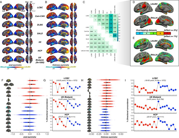
Population-level asymmetry of the cerebral cortex.
(A) Mean areal and (B) thickness asymmetry in each dataset. Warm and cold colours depict leftward and rightward asymmetry, respectively. (C) Spatial overlap (Pearson’s r) of the unthresholded maps between datasets for areal (lower matrix) and thickness asymmetry (upper). (D) Overlapping effects across datasets were used to delineate clusters exhibiting population-level areal (lower threshold = 5%) and (E) thickness asymmetry (lower threshold = 1%) based on a minimum 6-dataset overlap (black outlined clusters). (F, H) Raw distribution of the individual-level asymmetry index (AI) in adults extracted from clusters exhibiting areal and thickness asymmetry, respectively. Mean AI’s are in black, Raw distributions are shown for the LCBC (18–55 years) dataset with mixed effects data (cluster-wise outliers defined in lifespan analysis removed on a region-wise basis; Methods; Supplementary file 1E-F). X-axis denotes the AI of the average thickness and area of a vertex within the cluster. (G, I) Proportion of individuals with the expected directionality of asymmetry within each cluster exhibiting areal and thickness asymmetry, respectively, shown for the three largest adult datasets. The X-axes in G and I are ordered according to the clusters shown in F and H, respectively. Lat = lateral; Med = medial; Post = posterior; Ant = anterior; Sup = superior; Inf = inferior.
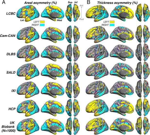
Significance of asymmetry effects across samples.
Significance for (A) areal and (B) thickness asymmetry across all samples. Note that because differences in sample size and test power affect the overall level of significance and consequently the FDR-correction, the visualization threshold is set to match the FDR-corrected significance level for each cortical metric in the first sample (LCBC; p<0.001). Warm and cold colours depict significance of leftward and rightward asymmetry, respectively. To permit more fine grained interpretation of anatomical correspondence, an outline of the (Destrieux et al., 2010) cortical atlas is overlain. Compare with effect sizes in Figure 1 in main paper.

Unthresholded maps.
Completely unthresholded significance maps of areal (leftmost 3 columns) and thickness (rightmost 3 columns) asymmetry ‘effects’ for the three largest samples. Desikan-Killiany atlas is overlain.
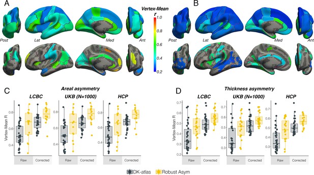
Comparison of vertex-wise and atlas-based asymmetry estimates.
To assess to what extent vertex-wise areal and thickness asymmetry estimates adhere to the anatomical boundaries of the Desikan-Killany (DK) atlas, we derived AI maps per subject and extracted a vertex × subject matrix. Then, within each of the 34 DK parcels we correlated the AI at each vertex with the parcel mean (i.e. the mean asymmetry across parcel vertices) and computed the mean correlation for each parcel. High correlations would be expected where atlas-derived parcels fit well to the underlying vertex-wise structure of cortical asymmetry. We then repeated this analysis using our set of robust asymmetry clusters. As a formal test, for each cortical metric the resulting coefficients were used as response variable in linear regressions with Cluster Type (DK parcels vs. Robust clusters) as predictor, controlling for cluster size (nVertices) and the Cluster Type × nVertices interaction. For areal asymmetry, the average vertex-mean correlations across all Desikan-Killiany (DK) parcels were r=0.53 ± [CI = 0.14] [LCBC], r=0.51 ± .14 [UK Biobank], and r=0.49 ± 0.15 [HCP], which respectively increased to r=0.65 ± 0.18, r=0.64 ± 0.18, and r=0.62 ± 0.19 for areal asymmetry clusters. For thickness, the average vertex-mean correlations across all DK parcels were r=0.36 ± 0.12 [LCBC], r=0.39 ± 0.12 [UK Biobank] and r=0.38 ± 0.12 [HCP], which respectively increased to r=0.47 ± 0.11, r=0.50 ± 0.11 and r=0.48 ± 0.12 for thickness asymmetry clusters. As would be expected, within parcel/cluster vertex-mean correlations were significantly lower in larger parcels/clusters. Linear regressions (size controlled) revealed a significant main effect of Cluster Type in all but one test (see Supplementary file 1D), confirming the visual impression that DK parcels conform poorly to the underlying asymmetry of cortex. (A–B) Average correlation between vertex-wise estimates of asymmetry within DK parcels to the mean across each parcel (top rows) and between vertex-wise asymmetry estimates within our robust clusters to the mean across each cluster (bottom rows), for areal (A) and thickness (B) asymmetry. The results on the surface are the average across the LCBC, UKB, and HCP datasets used in the vertex-wise analysis in main paper. The complete set of raw vertex-mean correlation coefficients correlated highly between all dataset-pairs for both areal [min r=0.97] and thickness asymmetry [min r=0.95]. (C–D) Vertex-mean correlation coefficients for areal asymmetry in DK parcels and robust asymmetry clusters, shown as raw values and after correcting for number of vertices in the parcel/cluster, for areal (C) and thickness asymmetry (D). Lat = lateral; Med = medial; Post = posterior; Ant = anterior.

HCP pipeline.
Thickness asymmetry results in the HCP dataset vary depending on the preprocessing pipeline. (A) Results from using the –hires argument to recon-all (as in main paper). We used this method to best harmonize preprocessing across cohorts whilst accounting for the higher resolution of HCP data. Shown again for comparison, the top row in A is akin to the results in the main paper (analyzed using cross-hemispheric registration methods) whereas the bottom row is the same data analyzed using standard parcellation methods (as in Figure 1—figure supplement 5). (B) Unthresholded thickness asymmetry results using the HCP preprocessed data subject to extra preprocessing steps and inputs, analyzed using cross-hemispheric registration methods (top row) and standard parcellation methods (bottom). (C) Results using the HCP preprocessed data when calculating thickness asymmetry on the fs_LR template. Warm and cold colours depict leftward and rightward asymmetry, respectively.
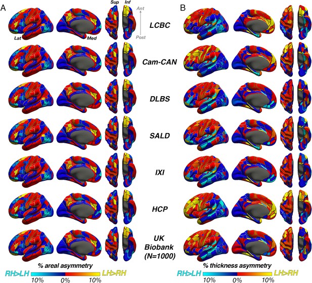
Unthresholded asymmetry effects analyzed using a standard brain atlas with no cross-hemispheric registration.
Mean (A) areal and (B) thickness asymmetry in each dataset analyzed using standard methods on the fsaverage template within parcels from the HCP multimodal brain atlas (Glasser et al., 2016). We used this atlas here because it appeared best suited to assess parcels that are homotopic. Warm and cold colours depict leftward and rightward asymmetry, respectively. Post = posterior; Lat = lateral; Med = medial; Ant = anterior; Sup = superior; Inf = inferior.
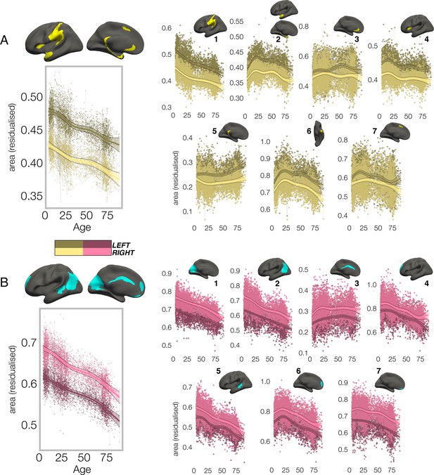
Lifespan trajectories of population-level areal asymmetry.
Homotopic lifespan trajectories of surface area in clusters exhibiting population-level (A) leftward (yellow plots; yellow clusters) and (B) rightward (pink plots; blue clusters) areal asymmetry (mm2). Larger plots on the left show the mean age trajectory across all clusters exhibiting leftward (top) and rightward (bottom) asymmetry. Note that the unit of measurement is the average surface area of a vertex within the cluster. Dark colours correspond to LH trajectories. All age trajectories were fitted using GAMMs. Data is residualized for sex, scanner and random subject intercepts. Clusters are numbered for reference. As outliers were removed on a region-wise basis (Methods), the number of observations underlying the plots range from 7862 to 7874 (see Supplementary file 1E).
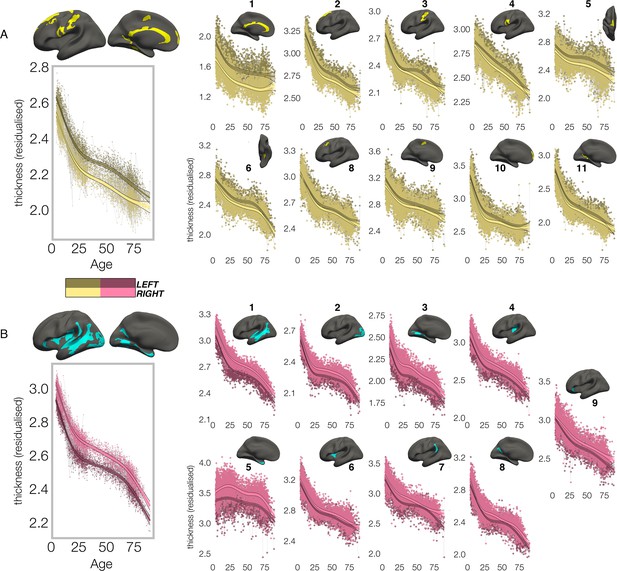
Lifespan trajectories of population-level thickness asymmetry.
Homotopic lifespan trajectories of cortical thickness in clusters exhibiting population-level (A) leftward (yellow plots; yellow clusters) and (B) rightward (pink plots; blue clusters) thickness asymmetry (mm). Larger plots on the left show the mean age trajectory across all clusters exhibiting leftward (top) and rightward (bottom) asymmetry. Dark colours correspond to LH trajectories. All age trajectories were fitted using GAMMs. Data is residualized for sex, scanner, and random subject intercepts. Clusters are numbered for reference. As outliers were removed on a region-wise basis (Methods), the number of observations underlying the plots range from 7856 to 7874 (see Supplementary file 1F).
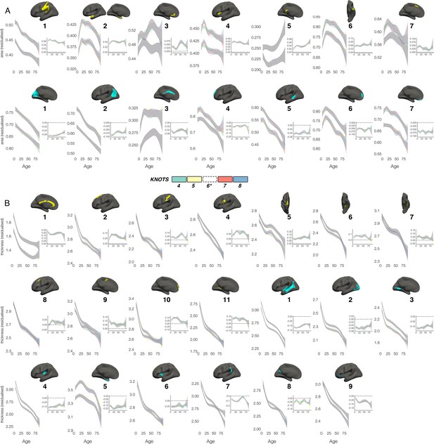
Knot comparison.
Lifespan trajectories of population-level (A) areal and (B) thickness asymmetries modelled with different smoothing parameters (number of knots 4–8, with the selected number of knots [*6] shown in black dotted outline). Grey indicates overlap. All age trajectories were fitted using GAMMs. Inset plots show absolute asymmetry trajectories (LH-RH) across life at the different smoothing parameters. As outliers were removed on a region-wise basis (Methods), the number of observations underlying the plots in A range from 7868 to 7874 (see Supplementary file 1E), and the number of observations underlying the plots in B range from 7856 to 7874 (see Supplementary file 1F).
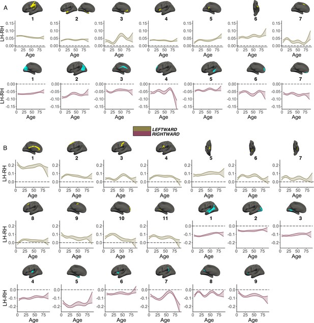
Smooth Age x Hemisphere interactions.
GAMM results for population-level (A) areal and (B) thickness asymmetries. A smooth Age × Hemisphere interaction was fitted to model asymmetry change across the lifespan. Specifically, GAMMs were used to compute the zero-centered age-trajectories of the left [s(LH-Age)] and right [s(RH-Age)] hemisphere for each cluster, and the asymmetry trajectory was computed as the difference between the two [s(LH-Age)-s(RH-Age)]. Gold and pink colours denote clusters defined by leftward or rightward asymmetry, respectively. For each cluster, the main effect of Hemisphere was added to visualize the lifespan trajectory of absolute asymmetry. Bands represent 95% confidence intervals. Note that all areal clusters show asymmetry trajectories that are significantly different from 0 (symmetry; dotted line) across the entire lifespan, and 19/20 thickness clusters were significantly asymmetric already by ~age 4. As outliers were removed on a region-wise basis (Methods), the number of observations underlying the plots in A range from 7868 to 7874 (see Supplementary file 1E), and the number of observations underlying the plots in B range from 7856 to 7874 (see Supplementary file 1F).
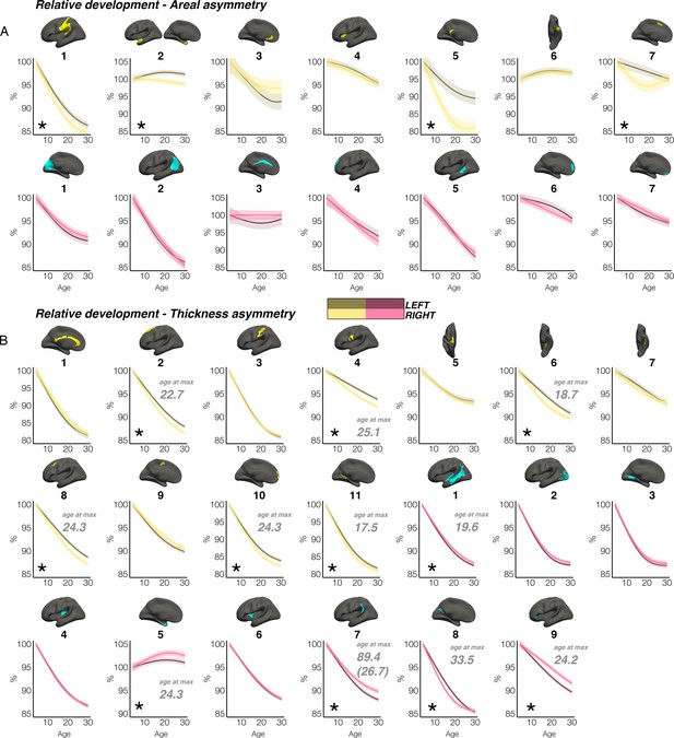
Relative developmental trajectories.
Relative developmental trajectories of homotopic cortical area and thickness in clusters exhibiting population-level (A) areal and (B) thickness asymmetry. Relative change was calculated by scaling the LH and RH fitted lifespan trajectories by the prediction at the minimum age (i.e. ~4 years). To highlight development, the x-axis covers the age-range 4–30 years, although relative change was calculated from full lifespan models (Methods). Darker trajectories indicate LH trajectories. Shaded areas indicate 95% CI. A relative difference in developmental change between hemispheres is suggested if the CI’s of relative LH and RH trajectories diverge to be non-overlapping (denoted with *). Note that for some areal asymmetries with suggestive relative hemispheric development, the data nevertheless was more indicative of stable and parallel trajectories (e.g. L1 and L2; see Figure 2), suggesting these indications of relative developmental hemispheric differences should be interpreted cautiously and in combination with the full lifespan GAMM trajectories shown in Figures 2 and 3, which contain inherent noise possibly due to the complexity of lifespan data (see Limitations). Note also that we report 10/20 relative developmental hemispheric differences for thickness asymmetry, as cluster R8 appeared to exhibit an initial faster thinning of the right hemisphere despite maintaining rightward thickness asymmetry throughout development (compare with Figure 3B). Where a relative developmental hemispheric difference was evident for thickness asymmetry, age at the point of maximum asymmetry across life is denoted in grey (calculated as the age of maximally non-overlapping CI’s). Since one cluster (R7) was estimated to exhibit maximum thickness asymmetry at age 89.4 (see Figure 3), age at maximum asymmetry for the developmental peak is also given in parentheses (Figure 3). As outliers were removed on a region-wise basis (Methods), the number of observations underlying the plots in A range from 7868 to 7874 (see Supplementary file 1E), and the number of observations underlying the plots in B range from 7856 to 7874 (see Supplementary file 1F). All lifespan age trajectories here were fitted using equivalent GAMMs as in the main paper, with the addition of a (scaled) ICV covariate (i.e. gamm(Y~s(Age, by = as.factor(hemi), k=6)+as.factor(hemi)+Sex + Scanner +ICV, data = DF, random = ~ (1 | ID))).
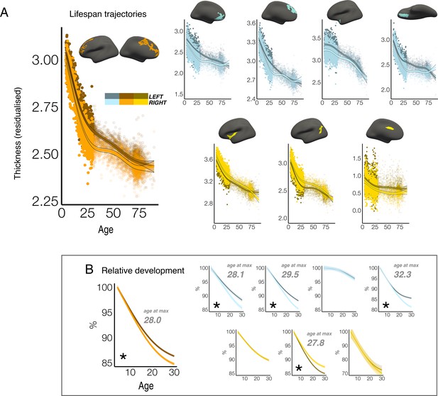
Lifespan thickness trajectories in regions exhibiting age-related change in asymmetry.
(A) Homotopic lifespan thickness trajectories in an alternative set of regions derived from a previous analysis (clusters from Roe et al., 2021; derived from vertex-wise analyses of age-related thickness asymmetry change in LCBC adult data [20–89 years]). Dark colours correspond to LH trajectories (colours correspond to clustering solutions in Roe et al., 2021). To highlight development, datapoints are semitransparent after age 30. Shaded areas indicate 95% CI. (B) Relative developmental LH and RH thinning from age 4–30. Plots correspond to the brain regions shown in A. Relative change was calculated by scaling the LH and RH fitted trajectories by the prediction at the minimum age (i.e. ~4 years). To highlight development, the x-axis covers the age-range 4–30 years, although the results are calculated from full lifespan models. Relative developmental change between hemispheres is suggested if the CI’s of relative LH and RH trajectories diverge to be non-overlapping (denoted with *). These indications of relative developmental hemispheric differences should be interpreted cautiously and in combination with the full lifespan GAMM trajectories shown in A, which contain inherent noise possibly due to the complexity of lifespan data (see Limitations). Where a relative developmental hemispheric difference was evident for thickness asymmetry, age at the point of maximum asymmetry across life is given, denoted in grey (calculated as the age of maximally non-overlapping CI’s). As outliers were removed on a region-wise basis (Methods), the number of observations underlying the plots are 7872, 7872, 7870, 7868, 7870, 7858, 7872, and 7872, respectively. All lifespan age trajectories here were fitted using equivalent GAMMs as in the main paper, with the addition of a (scaled) ICV covariate (i.e. gamm(Y~s(Age, by = as.factor(hemi), k=6)+as.factor(hemi)+Sex + Scanner +ICV, data = DF, random = ~ (1 | ID))).
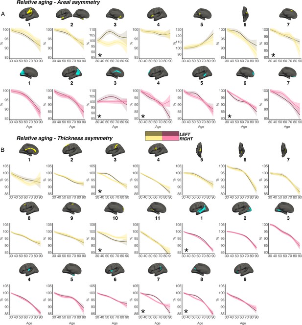
Relative aging trajectories.
Relative aging trajectories of homotopic cortical area and thickness in clusters exhibiting population-level (A) areal and (B) thickness asymmetry. Here, relative change was calculated by scaling the LH and RH fitted lifespan trajectories by the prediction at age 30 years. To highlight aging, the x-axis covers the age-range 30–89 years, although the results are calculated from full lifespan models. Darker trajectories indicate LH trajectories. Shaded areas indicate 95% CI. Relative aging-related change between hemispheres is suggested if the CI’s of relative LH and RH trajectories diverge to be non-overlapping (denoted with *). These indications of relative aging-related hemispheric differences should be interpreted cautiously and in combination with the full lifespan GAMM trajectories shown in Figures 2 and 3. As outliers were removed on a region-wise basis (Methods), the number of observations underlying the plots in A range from 7868 to 7874 (see Supplementary file 1E), and the number of observations underlying the plots in B range from 7856 to 7874 (see Supplementary file 1F). All lifespan age trajectories here were fitted using equivalent GAMMs as in the main paper, with the addition of a (scaled) ICV covariate (i.e. gamm(Y~s(Age, by = as.factor(hemi), k=6)+as.factor(hemi)+Sex + Scanner +ICV, data = DF, random = ~ (1 | ID))).
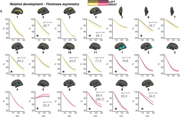
Relative developmental trajectories of homotopic cortical thickness in clusters exhibiting population-level thickness asymmetry.
To highlight development, the x-axis covers the age-range 4–30 years, although relative change was calculated from full lifespan models (Methods). Darker trajectories indicate LH trajectories. Shaded areas indicate 95% CI. A relative difference in developmental thinning rates between hemispheres is suggested if the CI’s of relative LH and RH trajectories diverge to be non-overlapping (denoted with *). These indications should be interpreted in combination with the full lifespan GAMM trajectories shown in Figure 3. Where relative hemispheric differences are indicated, age at the point of maximum thickness asymmetry across life is denoted in grey (Methods). Since one cluster (R7) was estimated to exhibit maximum thickness asymmetry at age 89.4 (see Figure 3), age at maximum asymmetry for the developmental peak is also given in parentheses (Figure 3). As outliers were removed on a region-wise basis (Methods), the number of observations underlying the plots range from 7856 to 7874 (see Supplementary file 1F).
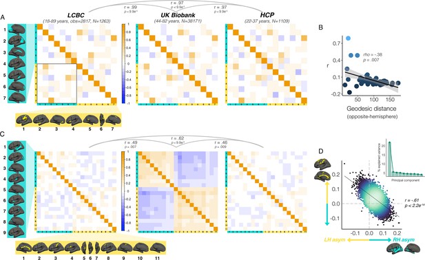
Interregional asymmetry correlations.
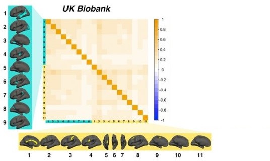
Interregional correlations between (A) areal asymmetries and (B) thickness asymmetries for each replication dataset (AI’s residualized for age, sex, scanner). Individual AI’s in rightward clusters are inversed, such that positive correlations reflect positive asymmetry-asymmetry relationships, regardless of direction of mean asymmetry in the cluster (i.e. higher asymmetry in the population-direction). Yellow and blue brain clusters/colours denote leftward and rightward asymmetries, respectively (clusters numbered for reference). A consistent covariance structure was evident both for areal (r ≥ 0.97) and thickness asymmetry (r ≥ 0.46; results above matrices). Black box in A highlights relationships between opposite-direction asymmetries (i.e. leftward vs rightward regions). (C) For areal asymmetry, asymmetry in opposite-direction cluster-pairs that were closer in cortex was more positively correlated (datapoints show cluster-pairs; geodesic distance in mm). (D) A single component explained 21.9% variance across thickness asymmetries in UKB (inset plot). Accordingly, we found a correlation of r=–0.61 (p<2.2e–16) in UKB between mean asymmetry across leftward clusters (Y-axis) vs. mean asymmetry across rightward clusters (X-axis; AI’s in rightward clusters inversed). Lines of symmetry (0) are in dotted grey (see also Figure 5—figure supplements 1–3).
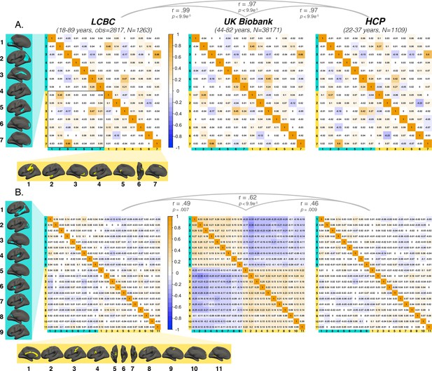
Annotated covariance matrices.
Interregional correlations between (A) areal asymmetries and (B) thickness asymmetries for each replication dataset (AI’s residualized for age, sex, scanner). Individual AI’s in rightward clusters are inversed, such that positive correlations reflect positive asymmetry-asymmetry relationships, regardless of direction of mean asymmetry in the cluster (i.e. higher asymmetry in the population-direction). Yellow and blue brain clusters/colours denote leftward and rightward asymmetries, respectively (clusters numbered for reference). A consistent covariance structure was evident both for areal (r ≥ 0.97) and thickness asymmetry (r ≥ 0.46; results above matrices). Black box in A highlights relationships between opposite-direction asymmetries (i.e. leftward vs rightward regions). Interregional correlations for thickness asymmetry in the lower left quadrant of UK Biobank matrix are visualized in Figure 5—figure supplement 2.
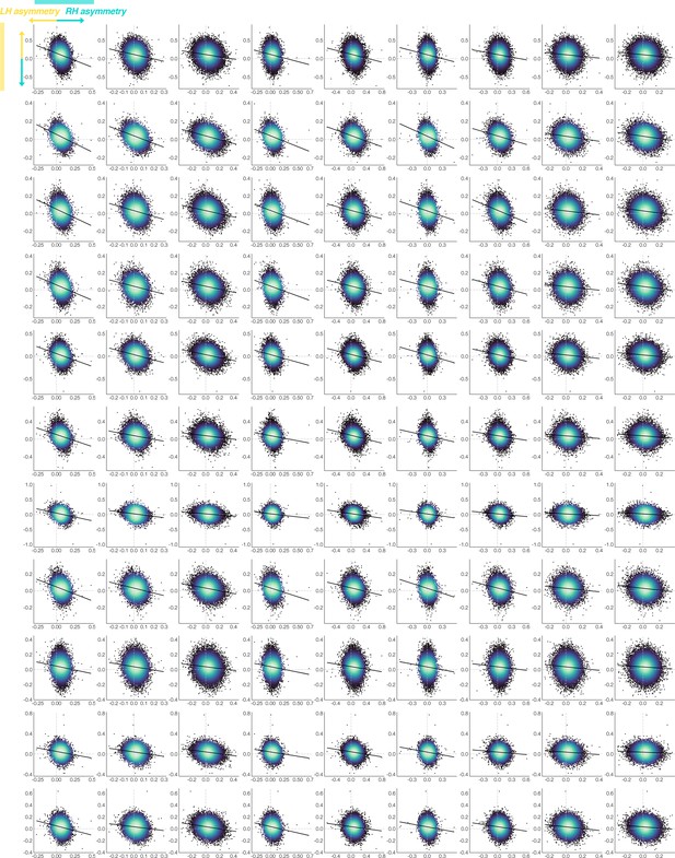
UK Biobank lower quadrant.
Thickness asymmetry interregional correlations between opposite-direction asymmetries (lower left quadrant of the UK Biobank correlation matrix in Figure 5—figure supplement 1; N=38,171) are visualized to describe whether negative asymmetry-asymmetry correlations pertained to reduced or reversed thickness asymmetry. Lines of symmetry (0) are shown in grey. X-axis and Y-show raw AI data after removing the fixed effects of age and sex. AI’s in rightward clusters are inversed, such that positive correlations would reflect positive asymmetry-asymmetry relationships regardless of direction of mean asymmetry in the cluster (i.e. higher asymmetry in the population direction). Order of cortical locations is in Figure 5—figure supplement 1.
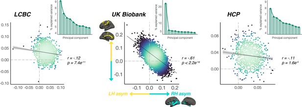
Global thickness asymmetry relationships.
Principal components analysis across AI’s in all leftward and rightward thickness asymmetry clusters revealed a single component explained 21.9% of the variance in UK Biobank, and there was evidence of a relatively stronger first component in LCBC and HCP (inset scree plots). Scatter plots show the partial correlation of the mean asymmetry across all leftward vs. all rightward clusters (means weighted by cluster size) plotted for each cohort, after AI’s were corrected for age, sex and (where applicable) scanner. Lines of symmetry (0) are shown as dotted grey. Individual AI’s in rightward clusters are inversed, such that positive correlations would reflect positive asymmetry-asymmetry relationships regardless of direction (i.e. higher asymmetry in the population direction).
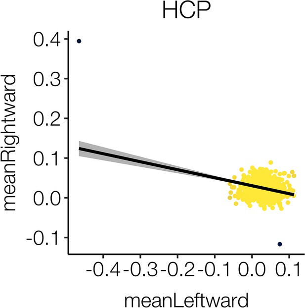
HCP outliers discarded.
Two outliers (black) were detected in the cortical thickness data of HCP and subsequently discarded for all analyses following the vertex-wise delineation of cortical asymmetry (in which their inclusion had negligible effect on the derived mean asymmetry maps). The plot shows mean thickness asymmetry across all leftward vs. mean thickness asymmetry across all rightward clusters.
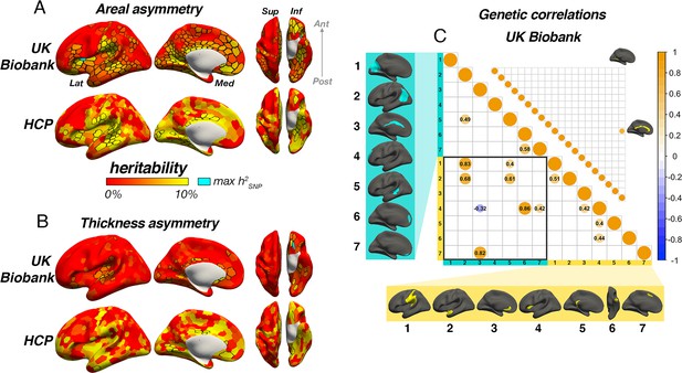
Asymmetry heritability.
Heritability of areal (A) and thickness asymmetry (B) estimated cortex-wide using SNP-based (UKB data; top rows) and twin-based methods (HCP data; bottom rows). Unthresholded effect maps are shown. Parcels in black outline show significance at p[FDR]<.05. Cyan parcels depict the point of maximum observed SNP-heritability (area h2=16.4%; thickness h2=16.6%). (C) Significant SNP-based genetic correlations (FDR-corrected) between areal (lower matrix) and thickness asymmetries (upper matrix). For area, SNP-based genetic correlations explained several phenotypic correlations (Figure 5A). For thickness, one pair survived FDR-correction (shown). See Figure 6—figure supplement 1 for comparison with genetic correlation estimates from the twin-based HCP sample. Individual AI’s in rightward clusters are inversed, such that positive genetic correlations reflect asymmetry-asymmetry genetic relationships, regardless of direction of mean asymmetry in the cluster (i.e. higher asymmetry in the population-direction). Yellow and blue brain clusters/colours denote leftward and rightward asymmetries, respectively (clusters numbered for reference).
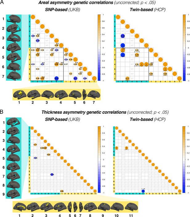
Genetic correlations exhibiting pre-corrected significance (p<0.05).
(A) SNP- and twin-based genetic correlations exhibiting pre-corrected significance (p<0.05) for areal asymmetry clusters and (B) thickness asymmetry clusters. Note that all clusters exhibiting significant SNP-based heritability (pre-corrected) were tested in both designs (78 tests for area; 55 for thickness; see Supplementary file 1H–I; NT = Not Tested). As such, some traits tested in the twin-based analysis were not found to exhibit significant twin-based heritability; hence, these results should be interpreted cautiously. Of note, a genetic correlation estimated at the boundary of parameter space (–1, 1) implies the genetic component of the phenotypes cannot be empirically distinguished. This is expected for phenotypes with a shared genetic basis, but may also reflect sampling variability of the estimator. Subscript denotes 95% CI (not estimated by GCTA; NA indicates that the optimizer could not find the confidence interval limit). ** denotes FDR-corrected significance. Individual AI’s in rightward clusters are inversed such that positive genetic correlations reflect asymmetry-asymmetry genetic relationships, regardless of direction of mean asymmetry in the cluster (i.e. higher asymmetry in the population-direction). Yellow and blue brain clusters/colours denote leftward and rightward asymmetries, respectively (clusters numbered for reference).
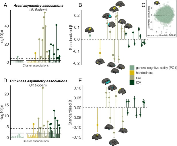
Asymmetry associations with general cognitive ability (first principal component [PC1]), handedness, sex, and intracranial volume (ICV) in UKB, in clusters exhibiting population-level areal (upper) and thickness asymmetry (lower).
(A, D) Significance of associations (negative logarithm; corrected [p<7.4e–5] and uncorrected threshold [p=0.01] shown by dotted and non-dotted line, respectively). X-axis displays the test for each cluster-association. As maximum sample size was used to test each association, effects of general cognitive ability were tested in separate models with fewer observations (N=35,198; separated association plots) than handedness, sex and ICV (N=37,569). (C) Visualization of the found association between leftward areal asymmetry in the large supramarginal cluster with general cognitive ability. The line of null association is shown for comparison (dotted) (B, E) Right plots denote effect sizes, 95% confidence intervals (error bars) and cortical location of associations surpassing Bonferroni-corrected significance. Individual AIs in rightward clusters were inversed. Right handers and females are coded 0, such that a negative effect for general cognitive ability / handedness / sex / ICV / reflects less asymmetry in higher cognition / left handers / males / larger brains. Associations with ICV are shown in Figure 7—figure supplement 2. Yellow and blue clusters denote leftward and rightward asymmetries, respectively.
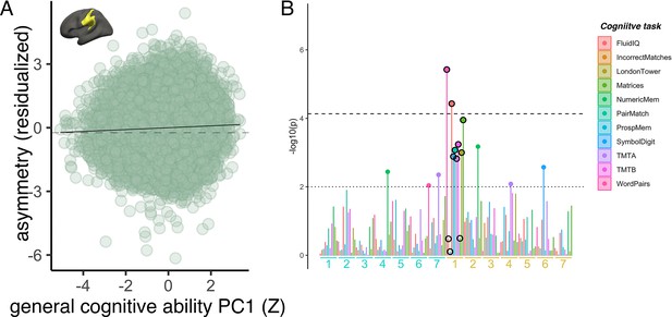
Cognitive associations.
(A) Association of reduced leftward areal asymmetry in the large supramarginal cluster upon general cognitive ability (PC1 across 11 cognitive tests). The line of null association is shown for comparison (dotted). (B) Post-hoc association tests between cognitive scores on the 11 separate tests in UKB and areal asymmetry in our 14 robust clusters (labelled under plot, leftward and rightward clusters in yellow and blue text, respectively). Black circled points highlight the association tests for the leftward cluster (visualized) wherein we find the association with general cognitive ability (i.e. PC1). Corrected (p<7.4e-5) and uncorrected threshold (p=0.01) shown by dotted and non-dotted line, respectively. As these tests are a post-hoc confirmation and not independent of the initial analysis using PC1 across tasks, the correction level is the same as in the main paper (note the association with PC1 survives regardless [p=7.4e-7]).
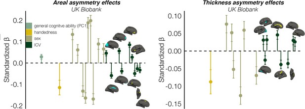
ICV effects (continuation of Figure 7).
Asymmetry effect sizes with general cognitive ability (first principal component [PC1]), handedness, sex, and intracranial volume (ICV) in UKB, in clusters exhibiting population-level areal (left) and thickness asymmetry (right). Effect sizes, 95% confidence intervals (error bars) and cortical location of associations with ICV surpassing Bonferroni-corrected significance (see Figure 7 for associated p-values). Individual AIs in rightward clusters were inversed. Right handers and females are coded 0, such that a negative effect size for handedness / sex / ICV / cognition reflects less asymmetry in left handers / males / larger brains / higher cognition. Blue and yellow clusters denote leftward and rightward asymmetry, respectively.
Additional files
-
Supplementary file 1
Supplementary tables A-M.
(A) Demographics of the samples used for each analysis. The number of unique participants (N unique), total observations (N obs), and number of scans constituting longitudinal observations (N longitudinal) is shown. Note that only the LCBC sample included longitudinal data (70% longitudinal coverage). * See Supplementary file 1C for further details of the HCP extended twin design used for heritability analysis. ** For analyses of SNP-heritability and *** associations with individual differences, to maximize power to detect effects subsets based on maximum data availability were taken from the N=38,171 UK Biobank base sample described here (i.e., all individuals with genotype data surpassing quality control; all individuals with available cognitive/handedness data; see Methods).
(B) MRI acquisition parameters by sample. TR = Repetition time; TE = Echo time; TI = Inversion time; FA = Flip angle; FOV = Field of view; 3D MPRAGE = three-dimensional magnetization prepared rapid gradient echo. * see available IXI imaging parameters here. **See UK Biobank brain imaging documentation here. (-) Not available/ found.
(C) Kinships of the extended twin design used for heritability analysis (HCP data). The number of observations of each pedigree type is given as well as the overall number of subjects per pedigree-type (N; Total N=1037). As no pedigree-type contained more than a single twin-pair, the number of monozygotic (MZ) and dizygotic (DZ) twin-pairs is reported per type. As all twins were same-sex, the ratio of female/male twin pairs is given per type.
(D) Linear regression results of the main effect of Cluster Type (i.e. Desikan-Killiany [DK] parcels v robust asymmetry clusters) upon the average correlation across vertex-mean correlations within parcels/clusters, controlling for cluster size (nVertices) and the Cluster Type × nVertices interaction. Average vertex-mean correlations were significantly higher for robust asymmetry clusters for areal asymmetry, and were significant or at trend-level for thickness asymmetry across each replication dataset.
(E) GAMM lifespan results for age-related change in areal asymmetry in robust asymmetry clusters (population-level areal asymmetries). A smooth Age × Hemisphere interaction [s(LH-Age)-s(RH-Age)] was modelled to determine whether asymmetry exhibited significant change across the lifespan. Significance of the smooth interaction (Bonferroni corrected; α<.05/14=.0036) is in bold. Effect size is denoted by Ω2. Hemisphere, Sex and Scanner (not shown) were additionally modelled as fixed effects covariates. Model fit is provided (r2 adjusted). The number of observations is given (including both hemispheres) after removing outliers on a cluster-wise basis (defined as observations >6 SD from the fitted trajectory of either hemisphere). Edf = estimated degrees of freedom (index of curve complexity).
(F) GAMM lifespan results for age-related change in thickness asymmetry in robust asymmetry clusters (population-level thickness asymmetries). A smooth Age × Hemisphere interaction [s(LH-Age)-s(RH-Age)] was modelled to determine whether asymmetry exhibited significant change across the lifespan. Significance of the smooth interaction (Bonferroni corrected; α<.05/20=.0025) is in bold. Effect size is denoted by Ω2. Hemisphere, Sex and Scanner (not shown) were additionally modelled as fixed effects covariates. Model fit is provided (r2 adjusted). The number of observations is given (including both hemispheres) after removing outliers on a cluster-wise basis (defined as observations >6 SD from the fitted trajectory of either hemisphere). Edf = estimates degrees of freedom (index of curve complexity).
(G) Heritability of global brain measures. Significant twin-based (HCP data) and SNP-based (UK Biobank data; N=31,433) heritability (h2) estimates are shown in bold, Bonferroni-corrected (P<8.3e-3 [.05/6]) separately for twin- and SNP-based estimates. Significant and high heritability estimates were observed for global brain measures of each hemisphere separately. For global asymmetry, twin-based heritability estimates were significant for both area and thickness, whereas only global areal asymmetry showed significant SNP-heritability in UK Biobank. e2=unique environmental effects + error; –2LL = minus 2 log likelihood index of model fit for AE (full model) and E (model without genetic parameter). Note that the correlations for DZ twins or sibling-pairs (rDZsibPairs) do not include data from third +siblings (sibs). Instead, we computed the correlation after concatenating data across all DZ twin-pairs, across twin1 (whether MZ or DZ) and sib1, or across sib1 and sib2 (where families had only siblings and no twins), all of which share 50% genetics on average. As there was always only one twin-pair in a family, the correlation for MZ twins (rMZ) is computed across all MZ twin-pair observations.
(H) Heritability of areal asymmetry in robust asymmetry clusters (population-level areal asymmetries). Significant twin-based (HCP data) and SNP-based (UK Biobank data; N=31,433) heritability (h2) estimates are shown in bold, Bonferroni-corrected (P<3.6e-3 [.05/14]) separately for twin- and SNP-based estimates. (van Kesteren and Kievit, 2021) Note the highest SNP-heritability was observed for areal asymmetry of the anterior insula (h2SNP = 18.6%). Note also that because the p-value was lower than the minimum in GCTA (P=0) we report P<1.78e-15 in the main text, which was the lowest numeric p-value in cortex-wide analyses. e2=unique environmental effects + error; –2LL = minus 2 log likelihood index of model fit for AE (full model) and E (model without genetic parameter). Note that the correlations for DZ twins or sibling-pairs (rDZsibPairs) do not include data from third +siblings. Instead, we computed the correlation after concatenating data across all DZ twin-pairs, across twin1 (whether MZ or DZ) and sib1, or across sib1 and sib2 (where families had only siblings and no twins), all of which share 50% genetics on average. As there was always only one twin-pair in a family, the correlation for MZ twins (rMZ) is computed across all MZ twin-pair observations.
(I) Heritability of thickness asymmetry in robust asymmetry clusters (population-level thickness asymmetries). Significant twin-based (HCP) and SNP-based (UK Biobank; N=31,433) heritability (h2) estimates are shown in bold, Bonferroni-corrected (P<2.5e-3 [.05/20]) separately for twin- and SNP-based estimates. e2=unique environmental effects + error; –2LL = minus 2 log likelihood index of model fit for AE (full model) and E (model without genetic parameter). Note that the correlations for DZ twins or sibling-pairs (rDZsibPairs) do not include data from third +siblings (sibs). Instead, we computed the correlation after concatenating data across all DZ twin-pairs, across twin1 (whether MZ or DZ) and sib1, or across sib1 and sib2 (where families had only siblings and no twins), all of which share 50% genetics on average. As there was always only one twin-pair in a family, the correlation for MZ twins (rMZ) is computed across all MZ twin-pair observations.
(J) Areal asymmetry associations. Results of linear regressions modelling the effects of individual differences (General Cognitive Ability, Handedness, Sex, and ICV) on asymmetry in population-level areal asymmetries in the full UK Biobank imaging sample with available cognitive data (imputed for no missing cognitive variables; N=35,198) or available handedness data (Handedness, Sex, ICV effects; N=37,569; Methods). Bold indicates Bonferroni-corrected significance (P<7.4e–5 [.01/136]). Right table shows significance of associations after controlling for additional brain-size related covariates following recent recommendations (Williams et al., 2022).
(K) Thickness asymmetry associations. Results of linear regressions modelling the effects of individual differences (General Cognitive Ability, Handedness, Sex, and ICV) on asymmetry in population-level thickness asymmetries in the full UK Biobank imaging sample with available cognitive data (imputed for no missing cognitive variables; N=35,198) or available handedness data (Handedness, Sex, ICV effects; N=37,569; Methods). Bold indicates Bonferroni-corrected significance (P<7.4e–5 [.01/136]). Right table shows significance of associations after controlling for additional brain-size related covariates following recent recommendations (Williams et al., 2022).
(L) Weightings of principal components across the 11 core cognitive variables in UK Biobank used here and cumulative variance explained.
(M) Dataset access information.
- https://cdn.elifesciences.org/articles/84685/elife-84685-supp1-v2.xlsx
-
Supplementary file 2
Cortical asymmetry and heritability maps (zipped folder).
- https://cdn.elifesciences.org/articles/84685/elife-84685-supp2-v2.zip
-
MDAR checklist
- https://cdn.elifesciences.org/articles/84685/elife-84685-mdarchecklist1-v2.docx


