Reconstructing the transport cycle in the sugar porter superfamily using coevolution-powered machine learning
- Department of Applied Physics, Science for Life Laboratory, KTH Royal Institute of Technology, Sweden
- Department of Biochemistry and Biophysics, Science for Life Laboratory, Stockholm University, Sweden
Figures
Figure 1
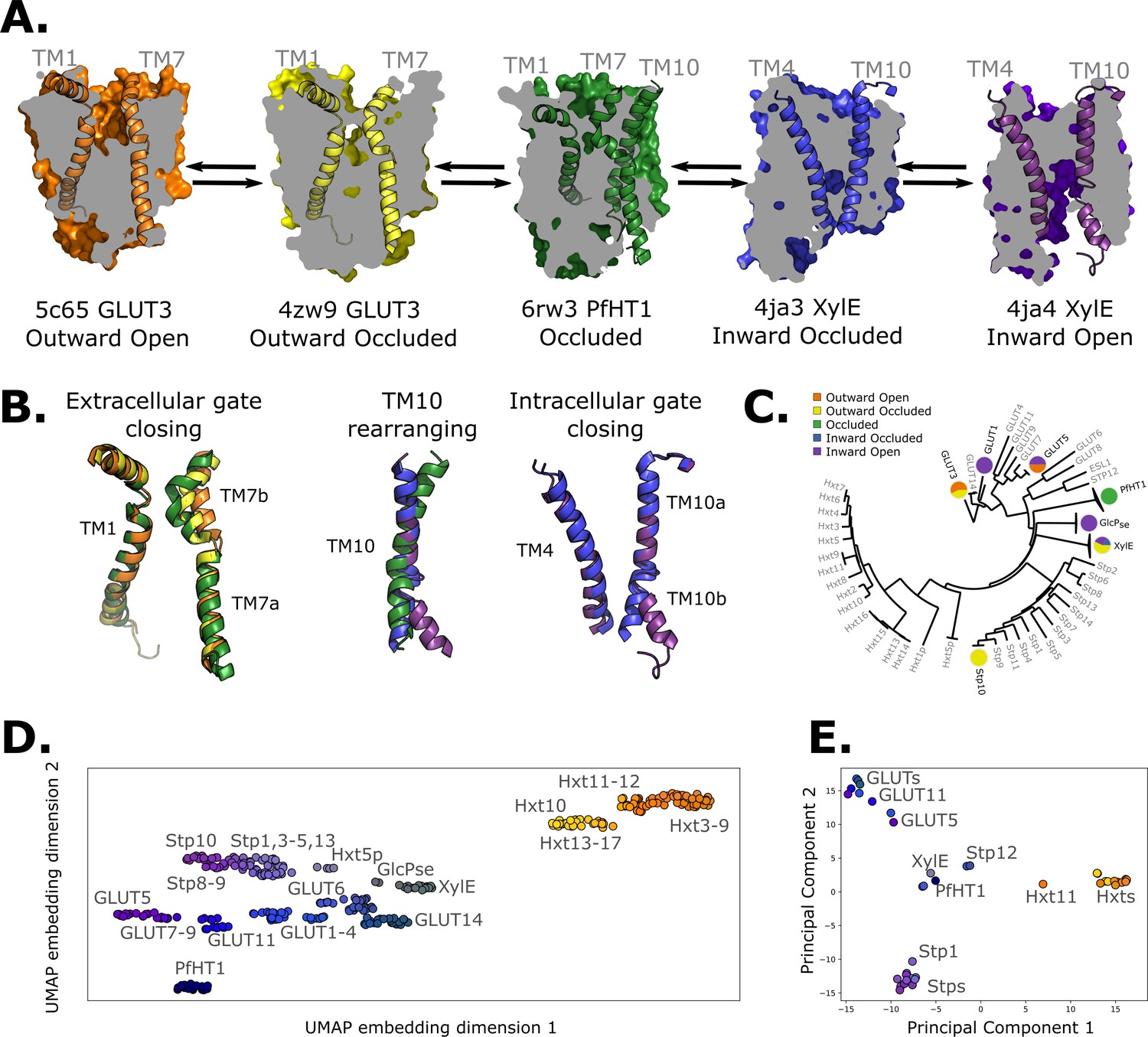
Available structural and evolutionary information.
(A) Clipped surfaces of representative structures of each functional state arranged according to the conformational cycle of sugar transporters (SPs). Note the alternating access to the intra- and extracellular solvents throughout the cycle. The gating helices TM7 and TM10 are shown in their cartoon representations, as well as their partners TM1 and TM4. (B) Cartoon representations of the primarily changing molecular features over the conformational cycle. First, the TM7b bends, then breaks when transition from the outward open to the occluded state through the outward-occluded state. In the rocker-switch motion, the TM10 helix rearranges to accommodate the rocking motion, after which the intracellular gate opens to form the inward open state. (C) The phylogenetic tree of the SP family, based on a multiple sequence alignment calculated by the MUSCLE algorithm. Tree generated using iTOL. The available experimental structures for each branch are highlighted as colored circles in the proportions that they appear in. The subfamilies represented in this tree are the mammalian sugar transporters (GLUTs), the bacterial and parasitic outliers (PfHT1, XylE, and GlcPse), the plant SPs, and the fungal hexose transporters (HXTs). Sequences were retrieved from UniProtKB. (D) A 2D embedding of the SP family in sequence space, using as similarity measure scores from the BLOSUM62-derived distance matrix. The embedding displays the phylogenetic distance between different branches of the sugar transporter family and are labeled as dots, colored according to their phylogenetic proximity. (E) Principal component analysis (PCA) projection of the available AlphaFold2 models in the SP family using as features residue–residue distances. SPs cluster according to phylogenetic proximity rather than conformational state.
Figure 2
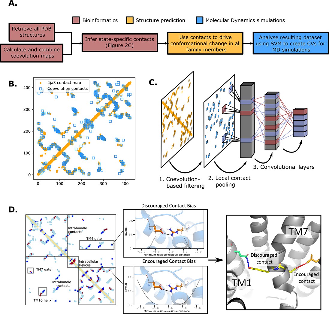
The state-specific structure prediction method.
(A) Summarized pipeline for obtaining a description of the conformational change in sugar transporters, colored by which technique is predominantly used. (B) An overlay of the top 200 coevolving residue pairs (blue) and the experimental contact map of the bacterial XylE structure 4ja3 in an inward-occluded state (orange). The secondary structure contacts from the coevolutionary analysis were omitted. (C) The architecture of the neural network used to train to predict conformational states from contacts between residue pairs. The first step consists in filtering out the low-coevolving contacts by the coevolution-based filtering, after which a restricted convolutional layer works to pool together close contacts in 4 × 4 grids, to account for the fact that contacts between adjacent positions often serve similar functions. Then, two unrestrained convolutions connect the aforementioned layer to the hidden layer and to the five-dimensional output layer, each node representing a single conformational state. (D) The bias application. The highly encouraged and discouraged contacts are translated into Ambiguous Constraint and Multi Constraint type biases in the RosettaMP fastrelax module, with the functional forms displayed in the middle panel. Using as input AlphaFold2 models of each member in the family, the biases are applied and the energy is minimized in a Monte-Carlo fashion, repeated to generate 100 models. The final structure is chosen as the model with the lowest energy score value.
Figure 3
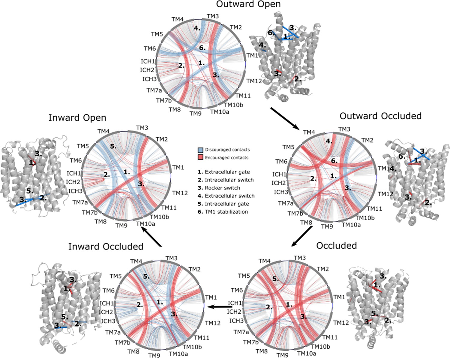
Network representations of the state-specific contact maps from the layer-wise relevance backpropagation (LRP) analysis of the trained neural network.
Nodes are labeled by the helix they are a part of, and the edges are colored by their sign in the LRP – blue represents discouraged contacts, and red represents encouraged contacts. Consensus contact maps of all states are shown in light gray in the background. Residue bundles that are encouraged or discouraged in a concerted manner (as revealed by their high importance in the pooling hidden layer of the neural network, Table 2) are highlighted with thick lines.
Figure 4
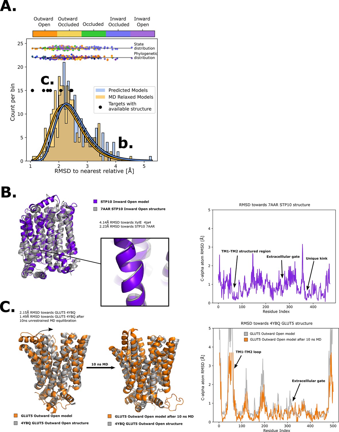
Quality of structure prediction of state-specific models of SPs.
(A) Histogram of root mean squared deviation (RMSD) of the structural models (Rosetta, blue and molecular dynamics [MD] relaxed, orange) from their closest relative in the same conformational state. The distributions of the MD-relaxed structures colored according to state and phylogeny (see color definition in Figure 1C) are shown above the histogram. Additionally, the targets with available experimental structures are indicated with black dots. (B) Alignment between STP10 inward open model and the newly solved 7AAR STP10 structure in the same conformational state. A helical kink not present in any experimentally determined structure so far is shown as an example of a transporter-specific feature that is captured by our structure prediction protocol. The residue-wise RMSD between our model and the experimentally determined structures is shown to the right, where the TM1–TM2 loop, extracellular gate and the aforementioned unique kink are highlighted. (C) (left) Alignment between the GLUT5 outward-open model and an experimental structure of the same isoform in the same state (PDB ID 4YBQ). (right) Alignment between the MD-relaxed GLUT5 outward-open model and PDB 4YBQ. The residue-wise RMSD between the MD models and the experimental structure is shown to the right, where the regions improved after 10 ns MD simulations are highlighted and labeled.
Figure 5 with 7 supplements
The entire conformational cycle is captured by accelerated weight histogram simulations.
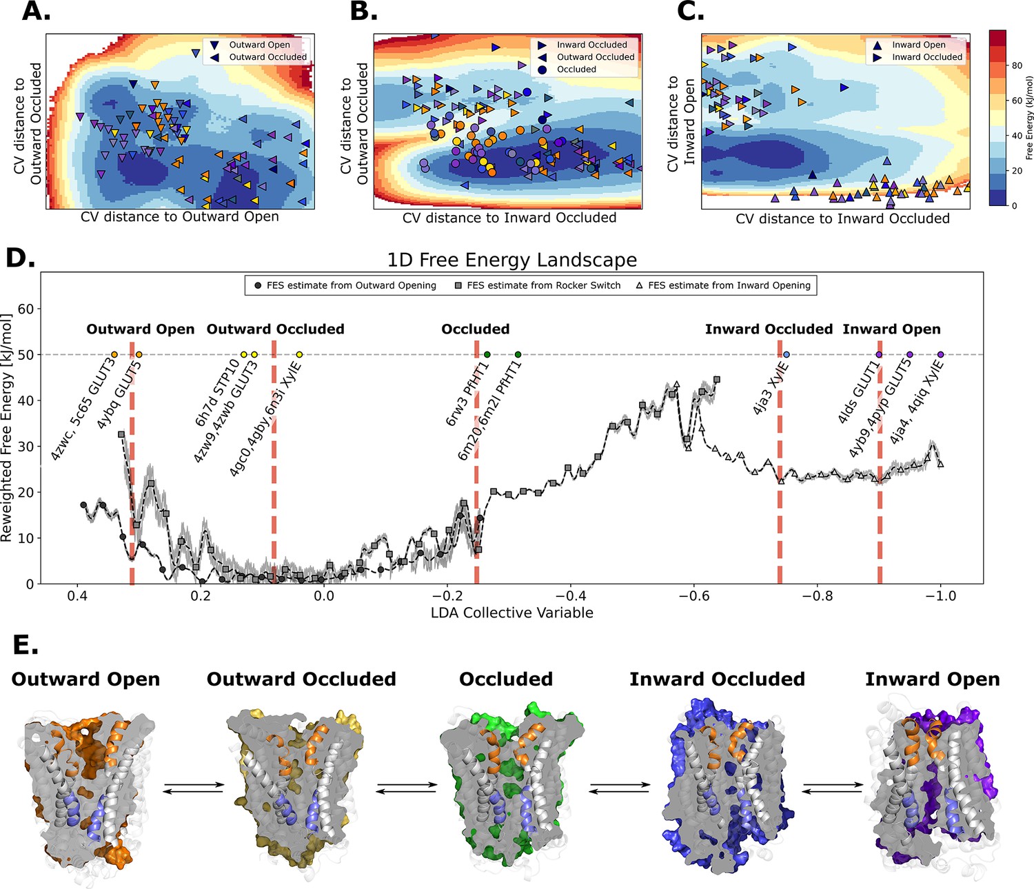
(A) Free-energy landscape of the outward opening process. The most populated free-energy basins are labeled according to annotation based on visual inspection and root mean squared deviation (RMSD) calculations of snapshots from the basins to the available experimentally determined structures. Projections of models of the outward-open and outward-occluded models of the various SPs are shown as symbols colored according to Figure 1D. Note that many outward-occluded models fall in the basin representing the occluded state, most likely because of the small structural difference between a bent and broken TM7b helix. (B) Free-energy landscape of the rocker-switch process. Representation as in A. Note that although not trained on the occluded models, models mostly either fall in the barrier region or in the GLUT5 occluded basin. (C) Free-energy landscape of the inward opening process. Representation as in A. (D) 1D free-energy landscape of the full conformational change, determined by reweighting the local free-energy estimates of panels A–C (labeled with different shapes) on a globally trained discriminative collective variable (see methods). The estimated point-wise error of the free-energy estimate is shown in gray. The experimentally solved structures were projected on the collective variable, and the lowest energy basin closest to the mean of each conformational state was extracted and analyzed and shown in panel E. (E) Representative structural models extracted from each of the most populated basins for each labeled state in panel D.
Figure 5—figure supplement 1
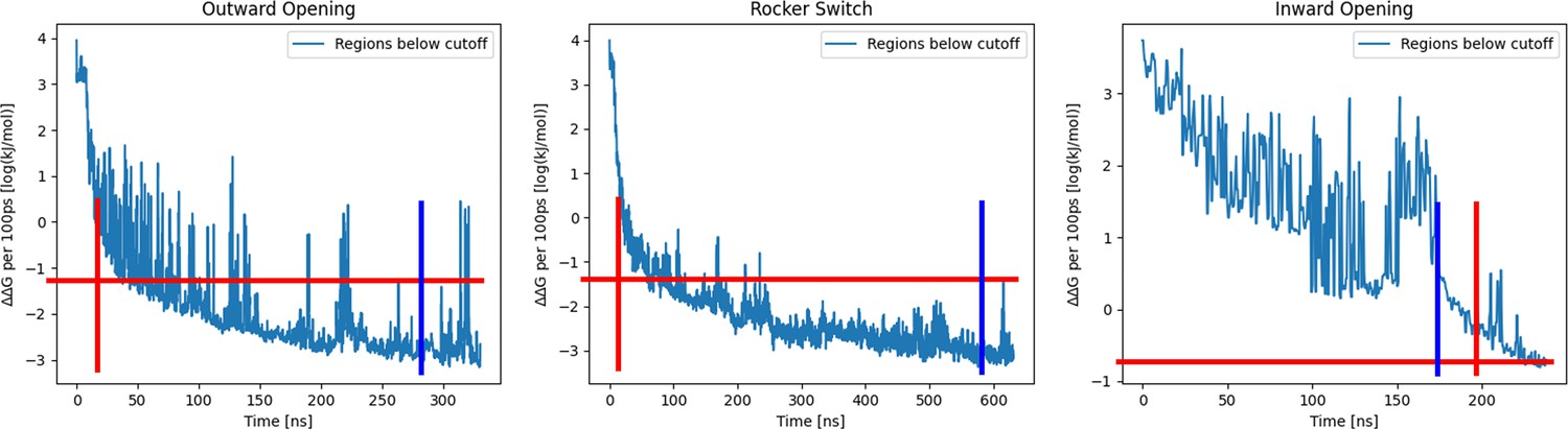
Convergence of accelerated weighted histogram (AWH) calculations.
Convergence was asserted by meeting two conditions: (1) Exiting the initial phase from AWH (vertical and horizontal crossing of red lines), and (2) Coordinate distribution at any point was not sampled more or less than twice as much as the mean coordinate distribution (vertical blue line). This was asserted separately on all processes. (left) Convergence plot of the outward opening process, showing the log10(ΔΔG) of the free-energy estimate over time. (middle) Convergence plot of the rocker-switch process, showing the log10(ΔΔG) of the free-energy estimate over time. (right) Convergence plot of the inward opening process, showing the log10(ΔΔG) of the free-energy estimate over time.
Figure 5—figure supplement 2
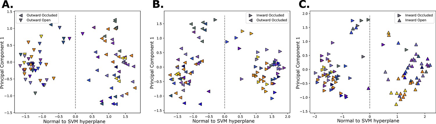
Collective variable learning.
Projected structures on the support vector machine (SVM)-derived vector (x-axis), and the first principal component from a principal component analysis (PCA) performed on models from adjacent states (y-axis). The classification border is at 0 along the SVM vector. The label of each structure is conveyed by the shapes, and the colors are according to Figure 1C. The processes considered are the outward opening (A), the rocker switch (B), and inward opening (C).
Figure 5—figure supplement 3
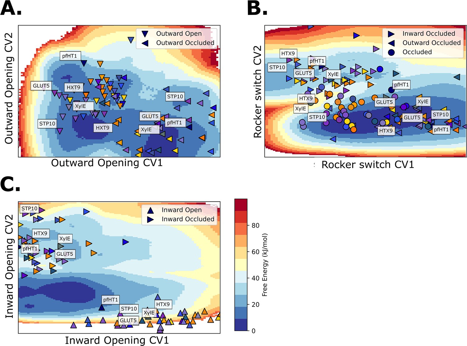
GLUT5, STP10, PfHT1, XylE, and HXT9 models projected on free-energy surfaces.
(A) Projection on the free-energy surface of the outward opening process. (B) Projection on the free-energy surface of the rocker-switch process. Note the different distributions of the occluded state structures (circles), which divide into two classes: GLUTs and pfHT1, and the rest of the sugar transporter family. Note also that the pfHT1 model falls on the barrier region of the GLUT5 transport cycle, similarly as in McComas et al., 2022. (C) Projection on the free-energy surface of the inward opening process.
Figure 5—figure supplement 4
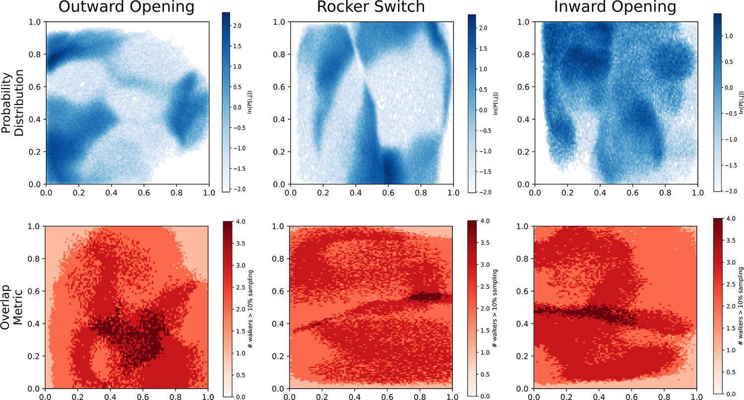
Overlap and probability distributions.
Top: Biased probability distribution of each accelerated weighted histogram (AWH) simulation, aggregated from all walkers. Bottom: Overlap between walkers. Instead of calculating how many walkers ever visit each bin, we only summed walkers that had a probability of over 10% of visiting said bin. The color signifies this overlap metric.
Figure 5—figure supplement 5
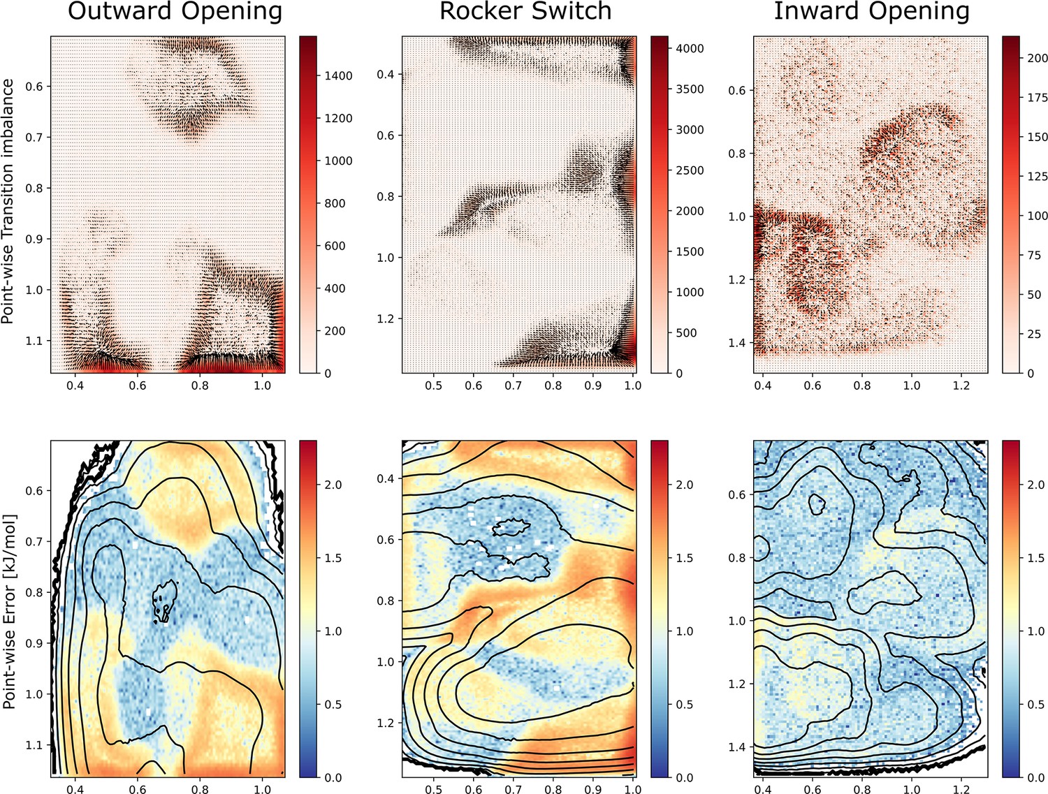
Transition imbalances and error estimation.
Top: Transition imbalances represented as vectors and colored by the transition matrix determinant (i.e., the ‘size’ of the imbalance which tightly correlates with the error) for each simulated process. The units are raw counts. Bottom: The estimated error calculated by dividing transition rates between neighboring bins, from which we obtained a measure of the probability imbalance which in turn was converted in the free-energy difference in kJ/mol. The error gives a local estimate of how far each point is estimated to be from a flat probability distribution. The black isocurves show the free-energy surfaces of Figure 5A–C.
Figure 5—figure supplement 6
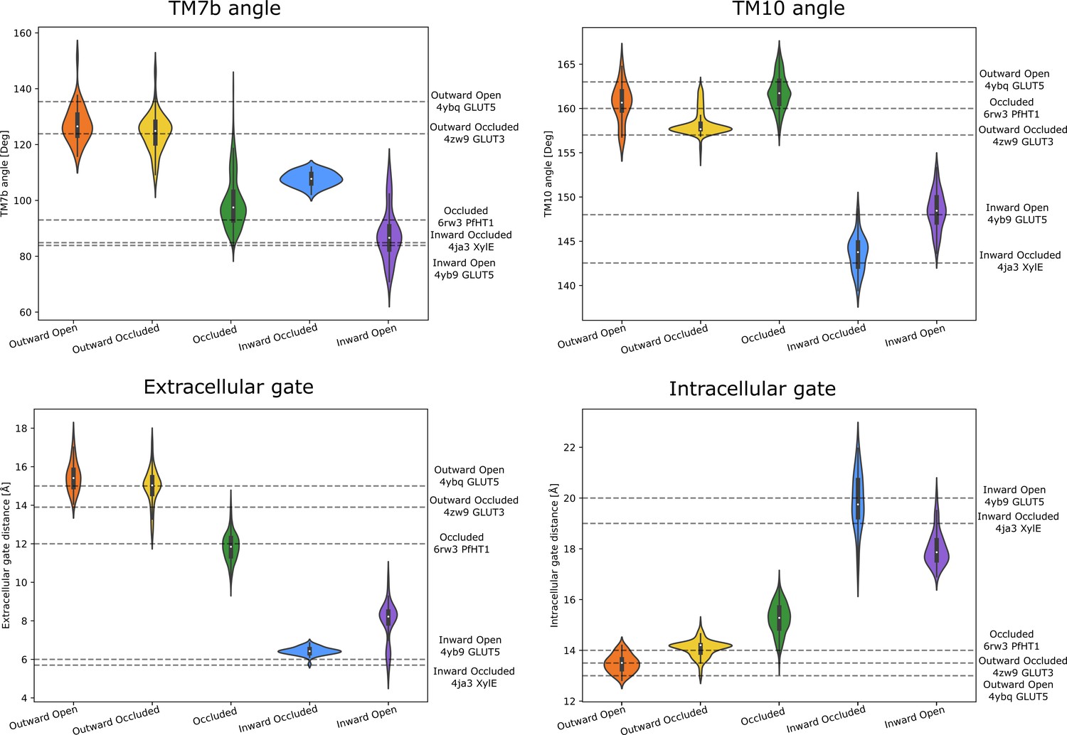
Observable distributions.
Measured distributions of the significantly populated wells. The horizontal lines are labeled according to the measured quantities in experimental reference structures of each state. The snapshots for the distributions were taken from the wells of Figure 5A–C that also overlapped well with the experimentally determined structures (Figure 5D). The scripts to measure and generate these quantities are found in the Zenodo repository.
Figure 5—figure supplement 7

Predicted structure stability analysis.
(A) Heavy-atom root mean squared deviation (RMSD) measured over time for each of the computationally predicted conformational states of GLUT5 used for accelerated weighted histogram (AWH) simulations. In the regions where the models deviate from the mean value, we measured the RMSD toward neighboring states to determine whether there had been conformational change. (B) Time evolution of the linear discriminant analysis (LDA) collective variable (CV) used for reweighting the free-energy landscapes along one coordinate. The distributions of the molecular dynamics (MD) simulations show increasing overlaps toward the end of the simulation, suggesting over 500 ns the structures relax into the main energy basins on either side of the large energetic barrier at around −0.5.
Figure 6 with 1 supplement
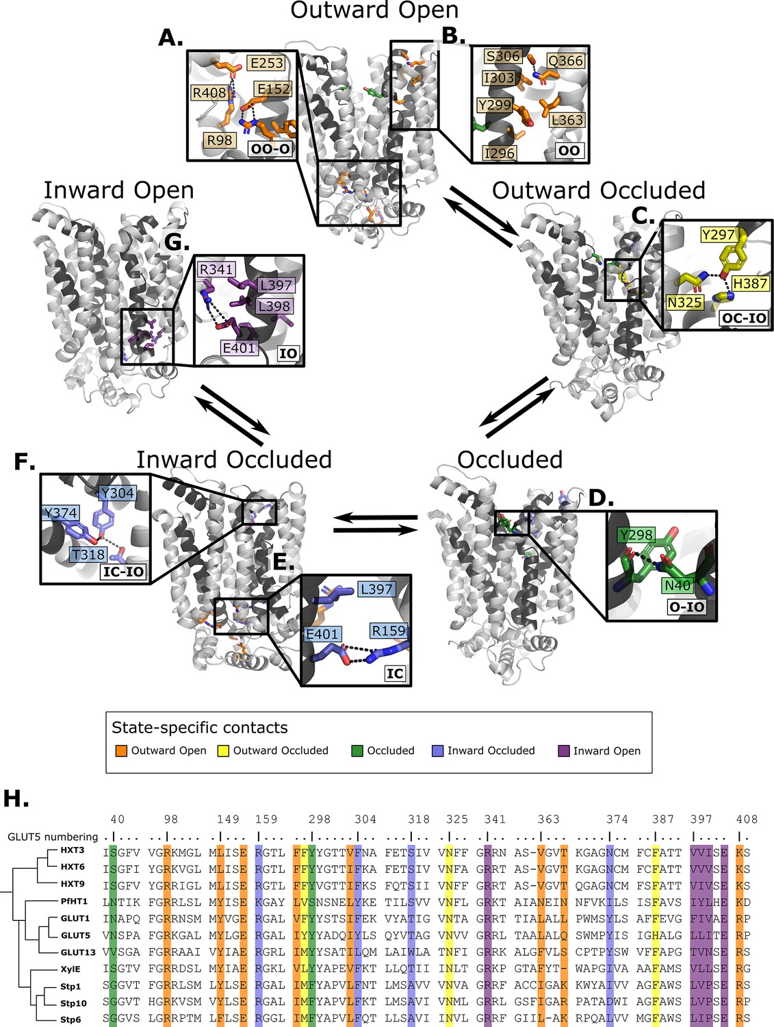
Summary of the structural determinants responsible for the cycling between adjacent conformational states.
Contacts are characteristic of the first conformation they appear in, but they can be maintained more or less throughout the cycle depending on the family members. The snapshots are of the GLUT5 models used as a representative member. The bottom right of every panel contains information about which states the contacts are present in (outward open/occluded [OO/OC], occluded [O], or inward open/occluded [IO/IC]). (A) Salt-bridge network at the intracellular side. This network is intact in all outward-facing states, but breaks during the rocker-switch motion (except for the E401/R159 contact, see panel E). (B) TM7b–TM9 interface responsible for stabilizing the outward-open conformation of TM7b, of which the hydrophobic contacts are only present in the outward-open state. (C) TM7b contact network responsible for promoting both the bent and broken conformation of TM7b. The position of N325 and H387 necessitates the rotation of TM7b which occludes the extracellular gate. (D) Backbone contact formed between TM7b and TM1, which is only possible when TM7b is completely broken. (E) TM10b–TM4 interactions that are the last occluding contacts to break before the intracellular gate opens. (F) TM10a–TM8 contacts responsible for stabilizing the new interbundle angle present in the inward-facing states. (G) Salt bridge and hydrophobic nexus responsible for stabilizing the inward-open conformation of TM10b, which fully unblocks the binding site from the intracellular side. (H) Multiple sequence alignment (MSA) of some representative members at positions shown throughout panels A–G. Since model training was performed on all predicted models using highly coevolving residue pairs as features, the type of interaction present in different subfamilies can be tracked in this MSA.
Figure 6—figure supplement 1
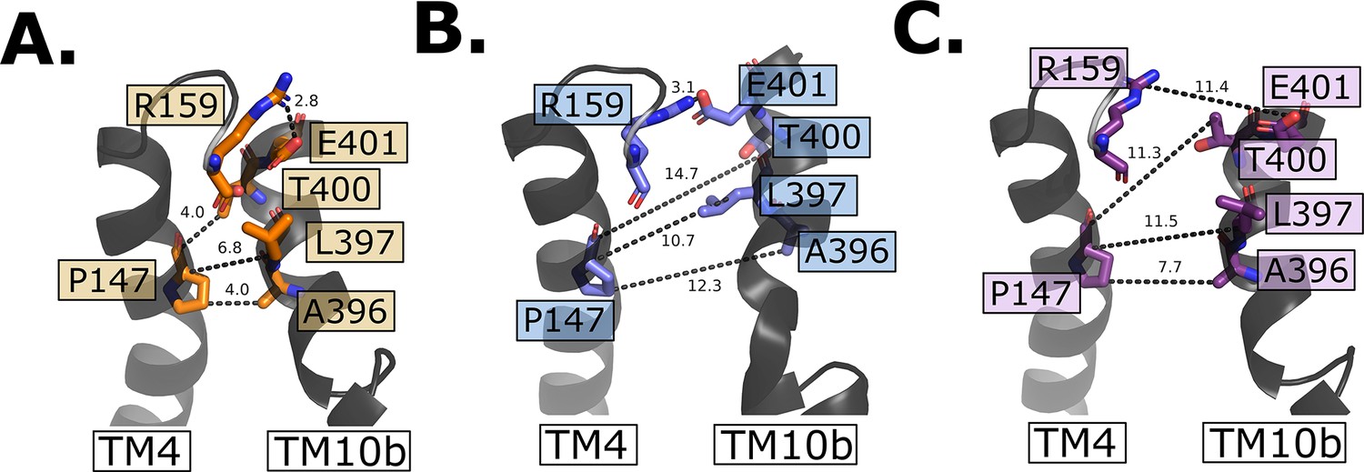
Intracellular gate evolution.
(A) Intracellular gate residues in the outward-open state. (B) Intracellular gate residues in the inward-occluded state. Note the intact salt bridge large opening between residue P147 and L396–A396. (C) Intracellular gate residues in the inward open state. Note the open gate and that now all interactions are broken between TM4 and TM10b.
Figure 7 with 1 supplement
Structural and evolutionary basis for proton coupling in the sugar transporter (SP) family.
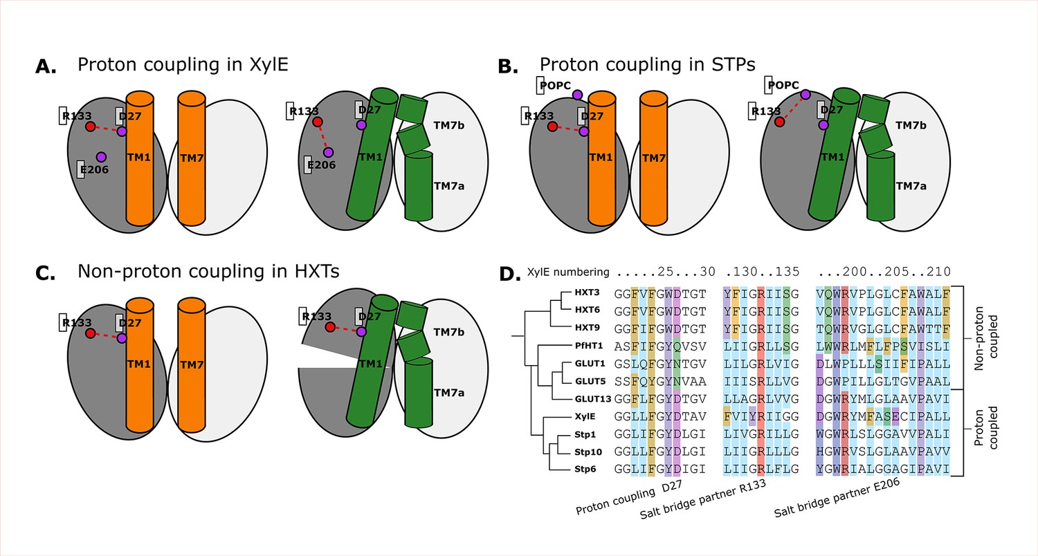
(A) Proposed cartoon model for proton coupling in XylE, showing the highlighted salt-bridge network rearrangements between the outward-open (orange) and occluded (green) conformational states. Note how these rearrangements facilitate the closure of the extracellular gate. (B) Proposed cartoon model for proton coupling in the SPs, showing the highlighted salt-bridge network rearrangements between the outward-open (orange) and occluded (green) conformational states. Note how these rearrangements facilitate the closure of the extracellular gate, and how R133 interacts with another latent salt-bridge partner than in XylE. (C) Proposed cartoon model explaining why HXTs generally lack proton coupling, showing the highlighted salt-bridge network rearrangements between the outward-open (orange) and occluded (green) conformational states. Note how the crucial R133–D27 contact can stay formed even in the occluded state due to a tilt of the entire helical bundle. (D) Multiple sequence alignment (MSA) of a selected subset of proton- and non-proton-coupled SPs, with residues labeled according to the XylE numbering.
Figure 7—figure supplement 1

Structural and evolutionary basis for proton coupling in the sugar transporter family with an atomic resolution.
(A) Comparison of the outward-open and occluded models of XylE. The proposed proton-coupling R133, D27, and E206 residues are highlighted. Note the salt-bridge rearrangement between states. (B) Comparison of the outward-open and occluded models of STP10. The analogous R133 and D27 (XylE numbering) residues are highlighted. (C) Comparison of the outward-open and occluded models of HXT9. The analogous R133 and D27 (XylE numbering) residues are highlighted. Although non-proton-coupled HXT9 carries the proton-coupling residues, but clearly, the interaction can still be formed in both states. (D) Comparison of the outward-open and occluded models of GLUT2. The analogous R133 and D27 (XylE numbering) residues are highlighted. Although non-proton-coupled GLUT2 does carry the proton-coupling residues, the coordination remains the same over the outward occlusion process, suggesting that TM7b undergoes larger conformational change in this isoform.
Tables
Table 1
Fraction of encouraged and discouraged contacts for each predicted state shown in Figure 3.
The fractions were calculated within the helical bundles (intrabundles 1 and 2), defined as spanning TM1–TM6 and TM7–TM12, respectively. Additionally, interbundle contacts between these two bundles were defined, along with the intracellular helix contacts (ICH1–5). The plus and minus signs denote the encouraged and discouraged contacts, respectively. The percentages concern the fraction of these contacts over all observed contacts in all members of the training set (all experimentally resolved structures).
| Intrabundle 1 | Intrabundle 2 | Interbundle | ICH | |||||
|---|---|---|---|---|---|---|---|---|
| + | − | + | − | + | − | + | − | |
| Out Open | 3.6% | 0.58% | 3.34% | 0.58% | 0.19% | 0.17% | 0.09% | 0.12% |
| Out Occ | 3.6% | 0.24% | 3.67% | 0.25% | 0.12% | 0.18% | 0.09% | 0.12% |
| Occ | 3.88% | 0.03% | 3.57% | 0.46% | 1.0% | 0.18% | 0.09% | 0.12% |
| In Occ | 3.64% | 0.31% | 3.40% | 0.77% | 0.2% | 0.16% | 0.09% | 2.9% |
| In Open | 3.52% | 0.27% | 3.64% | 0.33% | 0.09% | 0.20% | 1.12% | 3.0% |
Table 2
The most important residue contacts as identified by the neural network of Figure 3.
The residue numbering is relative to GLUT5. The contact bundles identified in Figure 3 were extracted from the first pooling layer, such that 5 × 5 connected residue interaction matrices were tracked. Here, the top contacts of these matrices are listed according to their raw layer-wise relevance backpropagation (LRP) value for each state. A negative sign on the LRP coefficients signifies a contact that is absent in a certain state.
| Outward open | |||
|---|---|---|---|
| Contact | Helices involved | Contact bundle | LRP |
| Y297-N40 | TM7b–TM1 | 1 | −3.21 |
| Y298-V39 | TM7b–TM1 | 1 | −2.34 |
| F430-L70 | TM2–TM11 (top) | 3 | −2.31 |
| W71-F432 | TM2–TM11 (top) | 3 | −2.24 |
| P193-P112 | TM6–TM3 | 4 | −2.01 |
| A177-A38 | TM5–TM1 | 6 | −1.7 |
| F412-L87 | TM2–TM11 (bottom) | 3 | 2.20 |
| N157-E337 | TM5–TM8 | 2 | 2.48 |
| A167-V336 | TM5–TM8 | 2 | 2.76 |
| Outward occluded | |||
| Contact | Helices involved | Contact bundle | LRP |
| F430-L70 | TM2–TM11 (top) | 3 | −3.09 |
| W71-F432 | TM2–TM11 (top) | 3 | −2.97 |
| Y298-V39 | TM7b–TM1 | 1 | −1.31 |
| Y297-N40 | TM7b–TM1 | 1 | 1.21 |
| F412-L87 | TM2–TM11 (bottom) | 3 | 2.12 |
| A177-A38 | TM5–TM1 | 6 | 2.48 |
| P193-P112 | TM6–TM3 | 4 | 2.58 |
| N157-E337 | TM5–TM8 | 2 | 2.94 |
| A167-V336 | TM5–TM8 | 2 | 2.97 |
| Occluded | |||
| Contact | Helices involved | Contact bundle | LRP |
| P147-L397 | TM4–TM10b | 5 | 1.13 |
| A396-P147 | TM4–TM10b | 5 | 1.19 |
| T400-P147 | TM4–TM10b | 5 | 1.43 |
| R159-E401 | TM4–TM10b | 5 | 2.19 |
| F412-L87 | TM2–TM11 (bottom) | 3 | 2.25 |
| F430-L70 | TM2–TM11 (top) | 3 | 2.46 |
| W71-F432 | TM2–TM11 (top) | 3 | 2.50 |
| N157-E337 | TM5–TM8 | 2 | 2.94 |
| A167-V336 | TM5–TM8 | 2 | 2.97 |
| Y298-V39 | TM7b–TM1 | 1 | 3.06 |
| Y297-N40 | TM7b–TM1 | 1 | 3.98 |
| Inward occluded | |||
| Contact | Helices involved | Contact bundle | LRP |
| P147-L397 | TM4–TM10b | 5 | −2.38 |
| A396-P147 | TM4–TM10b | 5 | −2.17 |
| T400-P147 | TM4–TM10b | 5 | −2.16 |
| F412-L87 | TM2–TM11 (bottom) | 3 | −1.96 |
| N157-E337 | TM5–TM8 | 2 | 1.23 |
| A167-V336 | TM5–TM8 | 2 | 1.48 |
| F430-L70 | TM2–TM11 (top) | 3 | 2.97 |
| W71-F432 | TM2–TM11 (top) | 3 | 2.98 |
| R159-E401 | TM4–TM10b | 5 | 3.15 |
| Y298-V39 | TM7b–TM1 | 1 | 3.25 |
| Y297-N40 | TM7b–TM1 | 1 | 3.27 |
| Inward open | |||
| Contact | Helices involved | Contact bundle | LRP |
| P147-L397 | TM4–TM10b | 5 | −3.12 |
| R159-E401 | TM4–TM10b | 5 | −3.01 |
| F412-L87 | TM2–TM11 (bottom) | 3 | −2.36 |
| N157-E337 | TM5–TM8 | 2 | −2.30 |
| A167-V336 | TM5–TM8 | 2 | −2.15 |
| A396-P147 | TM4–TM10b | 5 | −1.30 |
| T400-P147 | TM4–TM10b | 5 | −1.05 |
| F430-L70 | TM2–TM11 (top) | 3 | 2.34 |
| W71-F432 | TM2–TM11 (top) | 3 | 2.38 |
| Y298-V39 | TM7b–TM1 | 1 | 2.85 |
| Y297-N40 | TM7b–TM1 | 1 | 2.92 |
Table 3
Input parameters used for the accelerated weighted histogram (AWH) simulations.
The force constant determines the resolution of the free-energy surface and the bias toward the reference coordinate. The cover diameter determines the radius in collective variable (CV) space that has to be covered before a walker shares the bias at that point. The free-energy cutoff determined at which level sampling is deemed uninteresting. The convergence time is the simulation time per walker that was needed to achieve convergence according to the stated criteria.
| Diffusion constant (nm2/ps) | Force constant (kJ/mol/ nm2) | Cover diameter (nm) | Free-energy cutoff (kJ/mol) | Convergence time (ns/walker) | ||||
|---|---|---|---|---|---|---|---|---|
| CV1 | CV2 | CV1 | CV2 | CV1 | CV2 | |||
| Outward opening | 0.0005 | 0.001 | 10,000 | 50,000 | 0.4 | 0.4 | 60 | 374 |
| Rocker switch | 0.001 | 0.001 | 50,000 | 50,000 | 0.4 | 0.4 | 60 | 653 |
| Inward opening | 0.0005 | 0.0005 | 30,000 | 30,000 | 0.4 | 0.4 | 40 | 235 |
Additional files
Download links
A two-part list of links to download the article, or parts of the article, in various formats.
Downloads (link to download the article as PDF)
Open citations (links to open the citations from this article in various online reference manager services)
Cite this article (links to download the citations from this article in formats compatible with various reference manager tools)
Reconstructing the transport cycle in the sugar porter superfamily using coevolution-powered machine learning
eLife 12:e84805.
https://doi.org/10.7554/eLife.84805


