RatInABox, a toolkit for modelling locomotion and neuronal activity in continuous environments
- Sainsbury Wellcome Centre, University College London, United Kingdom
- Department of Cell and Developmental Biology, University College London, United Kingdom
- Department of Bioengineering, Imperial College London, United Kingdom
- Google DeepMind, United Kingdom
- Columbia University, United States
Figures
Figure 1
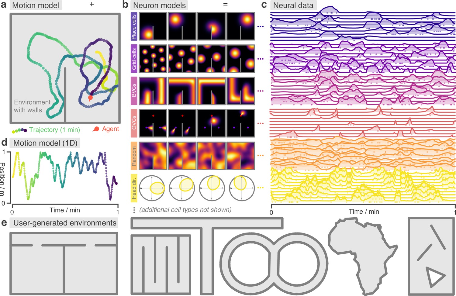
RatInABox is a flexible toolkit for simulating locomotion and neural data in complex continuous environments.
(a) One minute of motion in a 2D Environment with a wall. By default the Agent follows a physically realistic random motion model fitted to experimental data. (b) Premade neuron models include the most commonly observed position/velocity selective cells types (6 of which are displayed here). Users can also build more complex cell classes based on these primitives. Receptive fields interact appropriately with walls and boundary conditions. (c) As the Agent explores the Environment, Neurons generate neural data. This can be extracted for downstream analysis or visualised using in-built plotting functions. Solid lines show firing rates, and dots show sampled spikes. (d) One minute of random motion in a 1D environment with solid boundary conditions. (e) Users can easily construct complex Environments by defining boundaries and placing walls, holes and objects. Six example Environments, some chosen to replicate classic experimental set-ups, are shown here.
Figure 2
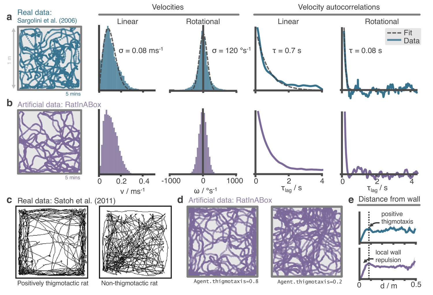
The RatInABox random motion model closely matches features of real rat locomotion.
(a) An example 5-min trajectory from the Sargolini et al., 2006. dataset. Linear velocity (Rayleigh fit) and rotational velocity (Gaussian fit) histograms and the temporal autocorrelations (exponential fit) of their time series’. (b) A sampled 5-min trajectory from the RatInABox motion model with parameters matched to the Sargolini data. (c) Figure reproduced from Figure 8D in Satoh et al., 2011 showing 10 min of open-field exploration. ‘Thigmotaxis’ is the tendency of rodents to over-explore near boundaries/walls and has been linked to anxiety. (d) RatInABox replicates the tendency of agents to over-explore walls and corners, flexibly controlled with a ‘thigmotaxis’ parameter. (e) Histogram of the area-normalised time spent in annuli at increasing distances, , from the wall. RatInABox and real data are closely matched in their tendency to over-explore locations near walls without getting too close.
Figure 3
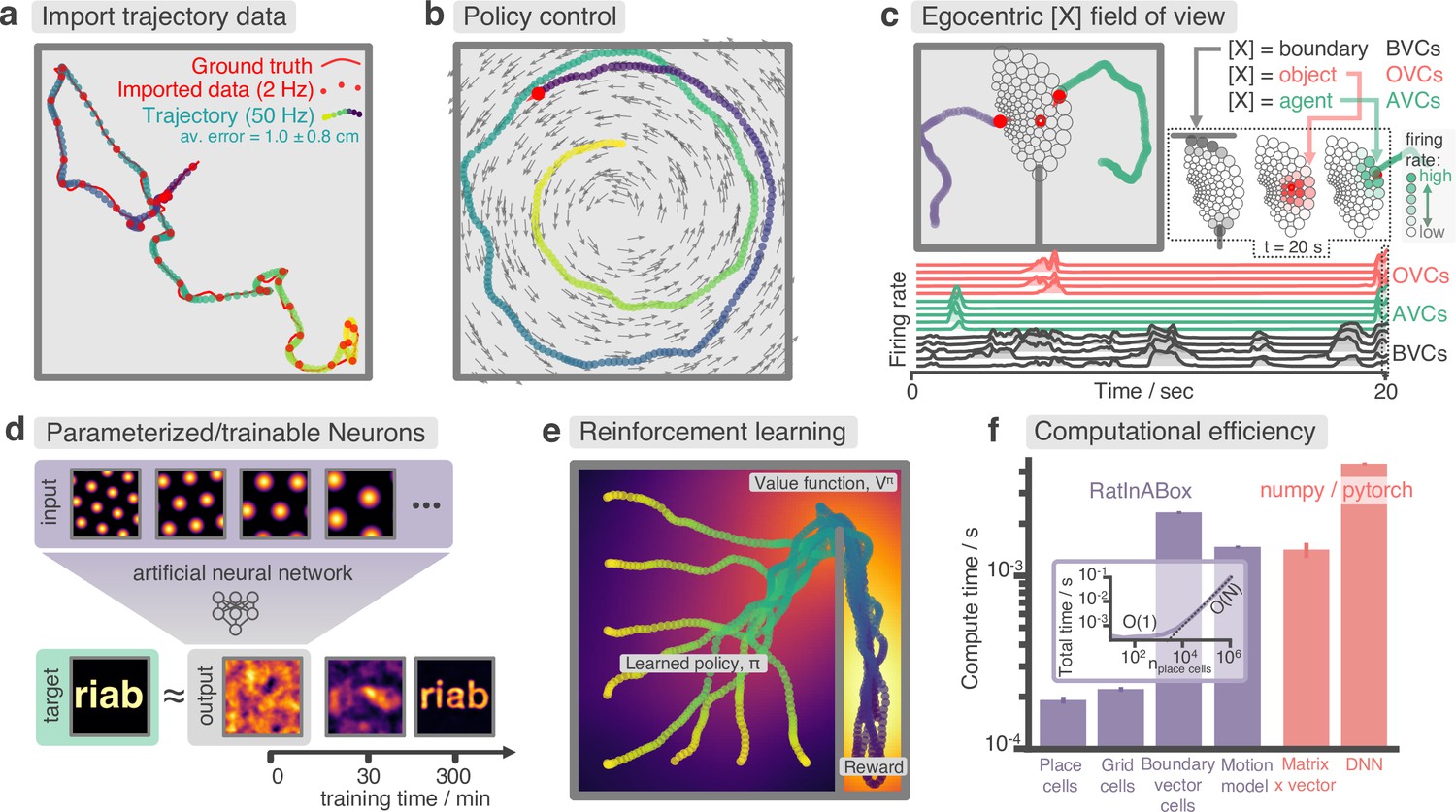
Advanced features and computational efficiency analysis.
(a) Low temporal-resolution trajectory data (2 Hz) imported into RatInABox is upsampled (‘augmented’) using cubic spline interpolation. The resulting trajectory is a close match to the ground truth trajectory (Sargolini et al., 2006) from which the low resolution data was sampled. (b) Movement can be controlled by a user-provided ‘drift velocity’ enabling arbitrarily complex motion trajectories to be generated. Here, we demonstrate how circular motion can be achieved by setting a drift velocity (grey arrows) which is tangential to the vector from the centre of the Environment to the Agent’s position. (c) Egocentric VectorCells can be arranged to tile the Agent’s field of view, providing an efficient encoding of what an Agent can ‘see’. Here, two Agents explore an Environment containing walls and an object. Agent-1 (purple) is endowed with three populations of Boundary- (grey), Object- (red), and Agent- (green) selective field of view VectorCells. Each circle represents a cell, its position (in the head-centred reference frame of the Agent) corresponds to its angular and distance preferences and its shading denotes its current firing rate. The lower panel shows the firing rate of five example cells from each population over time. (d) A Neurons class containing a feed forward neural network learns, from data collect online over a period of 300 min, to approximate a complex target receptive field from a set of grid cell inputs. This demonstrates how learning processes can be incorporated and modelled into RatInABox. (e) RatInABox used in a simple reinforcement learning example. A policy iteration technique converges onto an optimal value function (heatmap) and policy (trajectories) for an Environment where a reward is hidden behind a wall. State encoding, policy control and the Environment are handled naturally by RatInABox. (f) Compute times for common RatInABox (purple) and non-RatInABox (red) operations on a consumer grade CPU. Updating the random motion model and calculating boundary vector cell firing rates is slower than place or grid cells (note log-scale) but comparable, or faster than, size-matched non-RatInABox operations. Inset shows how the total update time (random motion model and place cell update) scales with the number of place cells.
Appendix 1—figure 1
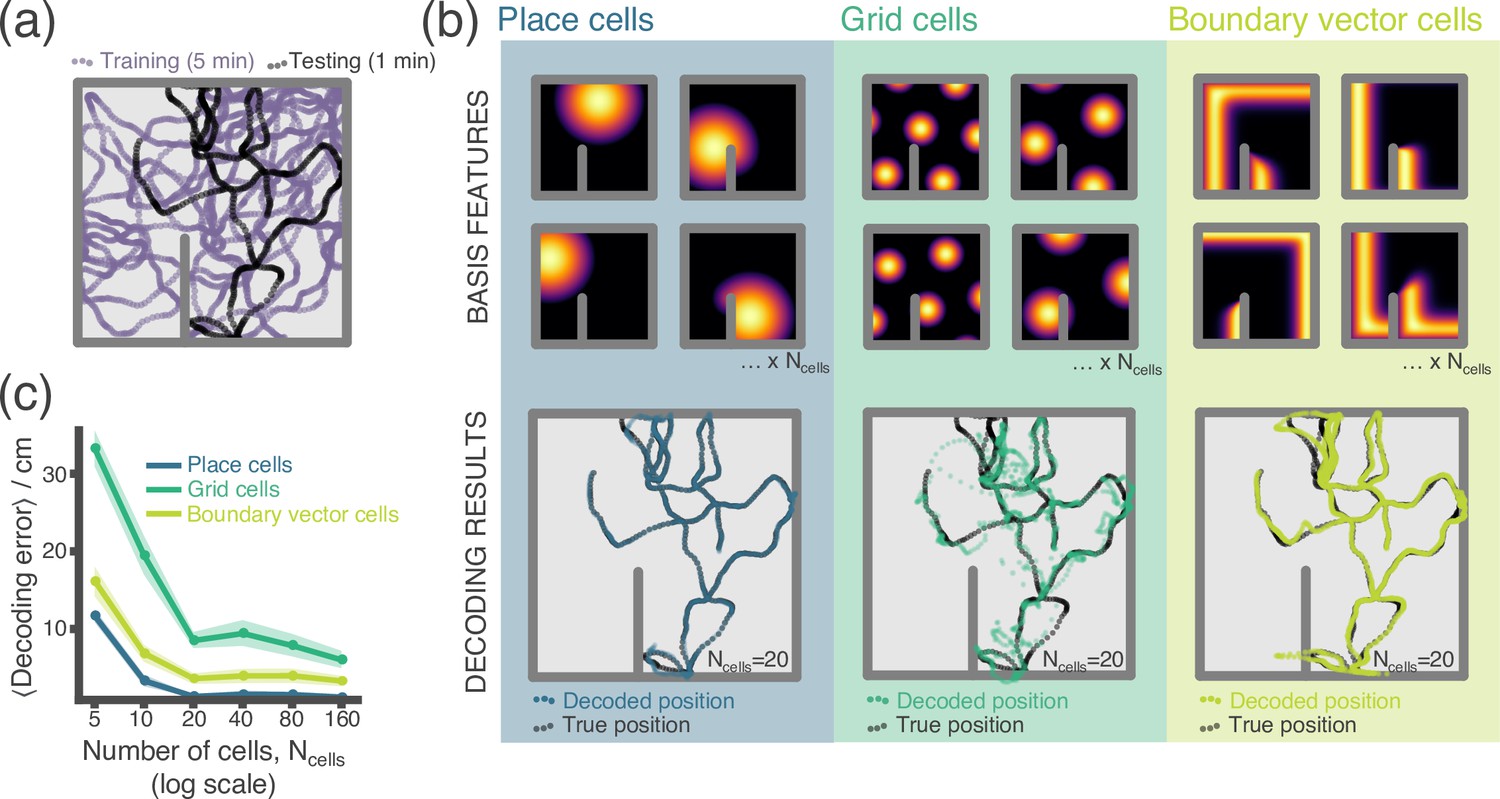
RatInABox used for a simple neural decoding experiment.
(a) Training (5 min) and testing (1 min) trajectories are sampled in a 1 m square environment containing a small barrier. (b) The firing rates of a population of cells, taken over the training trajectory, are used to fit a Gaussian Process regressor model estimating position. This decoder is then used to decode position from firing rates on the the unseen testing dataset. Top row shows receptive field for 4 of the 20 cells, bottom row shows decoding estimate (coloured dots) against ground truth (black dots). The process is carried out independently for populations of place cells (left), grid cells (middle) and boundary vector cells (right). (c) Average decoding error against number of cells, note log scale. Error region shows the standard error in the mean over 15 random seeds. A jupyter script demonstrating this experiment is given in the codebase GitHub repository.
Appendix 1—figure 2
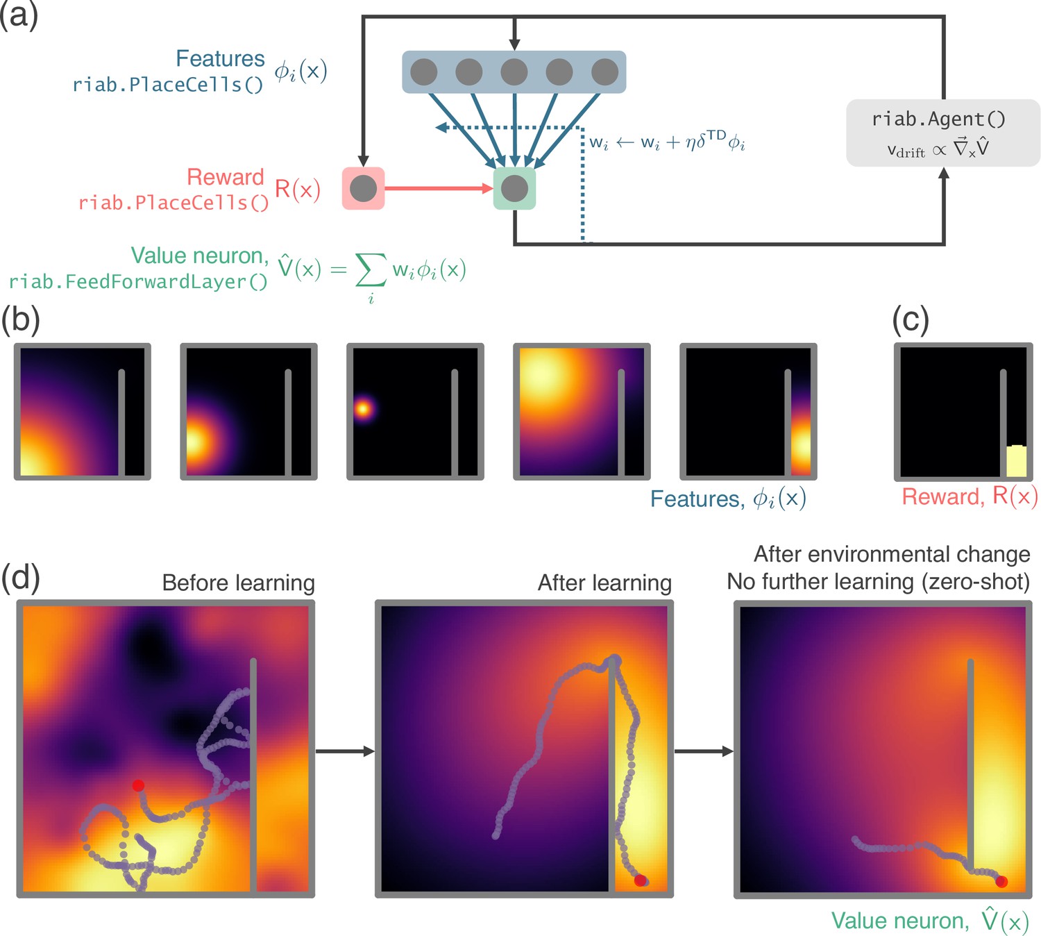
RatInABox used in a simple reinforcement learning project.
(a) A schematic of the 1 layer linear network. Using a simple model-free policy iteration algorithm the Agent, initially moving under a random motion policy, learns to approach an optimal policy for finding a reward behind a wall. The policy iteration algorithm alternates between (left) calculating the value function using temporally continuous TD learning and (right) using this to define an improved policy by setting the drift velocity of the Agent to be proportional to the gradient of the value function (a roughly continuous analog for the -greedy algorithm). (b) 1000 PlaceCells act as a continuous feature basis for learning the value function. (c) The reward is also a (top-hat) PlaceCell, hidden behind the obstructing wall. (d) A ValueNeuron (a bespoke Neurons subclass defined for this demonstration) estimates the policy value function as a linear combination of the basis features (heatmap) and improves this using TD learning. After learning the Agent is able to accurately navigate around the wall towards the reward (middle). Because PlaceCells in RatInABox are continuous and interact adaptively with the Environment when a small gap is opened in the wall place fields corresponding to place cells near this gap automatically bleed through it, and therefore so does the value function. This allows the Agent to find a shortcut to the reward with zero additional training. A jupyter script replicating this project is given in the demos folder GitHub repository.
Author response image 1

Tables
Table 1
Default values, keys and allowed ranges for RatInABox parameters.
* This parameter is passed as a kwarg to Agent.update() function, not in the input dictionary. ** This parameter is passed as a kwarg to FeedForwardLayer.add_input() when an input layer is being attached, not in the input dictionary.
| Parameter | Key | Description (unit) | Default | Acceptable range |
|---|---|---|---|---|
| Environment() | ||||
| dimensionality | Dimensionality of Environment. | "2D" | ["1D","2D"] | |
| Boundary conditions | boundary_conditions | Determines behaviour of Agent and PlaceCells at the room boundaries. | "solid" | ["solid", "periodic"] |
| Scale, | scale | Size of the environment (m). | 1.0 | |
| Aspect ratio, | aspect | Aspect ratio for rectangular 2D Environments; width = , height = . | 1.0 | |
| dx | Discretisation length used for plotting rate maps (m). | 0.01 | ||
| Walls | walls | A list of internal walls (not the perimeter walls) which will be added inside the Environment. More typically, walls will instead be added with the Env.add_wall() API (m). | [] | -array/list |
| Boundary | boundary | Initialise non-rectangular Environments by passing in this list of coordinates bounding the outer perimeter (m). | None | -array/list |
| Holes | holes | Add multiple holes into the Environment by passing in a list of lists, each internal list contains coordinates (min 3) bounding the hole (m). | None | -array/list |
| Objects | walls | A list of objects inside the Environment. More typically, objects will instead be added with the Env.add_object() API (m). | [] | -array/list |
| Agent() | ||||
| dt | dt | Time discretisation step size (s). | 0.01 | |
| speed_coherence_time | Timescale over which speed (1D or 2D) decoheres under random motion (s). | 0.7 | ||
| (2D) (1D) | speed_mean | 2D: Scale Rayleigh distribution scale parameter for random motion in 2D. 1D: Normal distribution mean for random motion in 1D (ms-1). | 0.08 | 2D: 1D: |
| speed_std | Normal distribution standard deviation for random motion in 1D (ms-1). | 0.08 | ||
| rotational_velocity_coherence_time | Rotational velocity decoherence timescale under random motion (s). | 0.08 | ||
| rotational_velocity_std | Rotational velocity Normal distribution standard deviation (rad s-1). | |||
| thigmotaxis | Thigmotaxis parameter. | 0.5 | ||
| wall_repel_distance | Wall range of influence (m). | 0.1 | ||
| s | walls_repel_strength | How strongth walls repel the Agent. 0=no wall repulsion. | 1.0 | |
| drift_to_random_ strength_ratio* | How much motion is dominated by the drift velocity (if present) relative to random motion. | 1.0 | ||
| Neurons() | ||||
| n | Number of neurons. | 10 | ||
| max_fr | Maximum firing rate, see code for applicable cell types (Hz). | 1.0 | ||
| min_fr | Minimum firing rate, see code for applicable cell types (Hz). | 0.0 | ||
| noise_std | Standard deviation of OU noise added to firing rates (Hz). | 0.0 | ||
| noise_coherence_time | Timescale of OU noise added to firing rates (s). | 0.5 | ||
| Name | name | A name which can be used to identify a Neurons class. | "Neurons" | Any string |
| PlaceCells() | ||||
| Type | description | Place cell firing function. | "gaussian" | ["gaussian", "gaussian_threshold", "diff_of_gaussians", "top_hat", "one_hot"] |
| widths | Place cell width parameter; can be specified by a single number (all cells have same width), or an array (each cell has different width) (m). | 0.2 | ||
| place_cell_centres | Place cell locations. If None, place cells are randomly scattered (m). | None | None or array of positions (length ) | |
| Wall geometry | wall_geometry | How place cells interact with walls. | "geodesic" | ["geodesic", "line_of_sight", "euclidean"] |
| GridCells() | ||||
| gridscale | Grid scales (m), or parameters for grid scale sampling distribution. | (0.5,1) | array-like or tuple | |
| -dist | gridscale_distribution | The distribution from which grid scales are sampled, if they aren’t manually provided as an array/list. | "uniform" | see utils.distribution_sampler() for list |
| orientation | Orientations (rad), or parameters for orientation sampling distribution. | (0,2π) | array-like or tuple | |
| -dist | orientation_distribution | The distribution from which orientations are sampled, if they aren’t manually provided as an array/list. | "uniform" | see utils.distribution_sampler() for list |
| phase_offset | Phase offsets (rad), or parameters for phase offset sampling distribution. | (0,2π) | array-like or tuple | |
| -dist | phase_offset_distribution | The distribution from which phase offsets are sampled, if they aren’t manually provided as an array/list. | "uniform" | see utils.distribution_sampler() for list |
| Type | description | Grid cell firing function. | "three_rectified_cosines" | ["three_rectified_cosines", "three_shifted_cosines"] |
| VectorCells() | ||||
| Reference frame | reference_frame | Whether receptive fields are defined in allo- or egocentric coordinate frames | "allocentric" | ["allocentric", "egocentric"] |
| Arrangement protocol | cell_arrangement | How receptive fields are arranged in the environment. | "random" | ["random", "uniform_manifold", "diverging_manifold", function()] |
| tuning_distance | Tuning distances (m), or parameters for tuning distance sampling distribution. | (0.0,0.3) | array-like or tuple | |
| -dist | tuning_distance_distribution | The distribution from which tuning distances are sampled, if they aren’t manually provided as an array/list. | "uniform" | see utils.distribution _sampler() for list |
| sigma_distance | Distance tuning widths (m), or parameters for distance tuning widths distribution. (By default these give and ) | (0.08,12) | array-like or tuple | |
| -dist | sigma_distance_distribution | The distribution from which distance tuning widths are sampled, if they aren’t manually provided as an array/list. "diverging" is an exception where distance tuning widths are an increasing linear function of tuning distance. | "diverging" | see utils.distribution _sampler() for list |
| tuning_angle | Tuning angles (), or parameters for tuning angle sampling distribution (degrees). | (0.0,360.0) | array-like or tuple | |
| -dist | tuning_angle_distribution | The distribution from which tuning angles are sampled, if they aren’t manually provided as an array/list. | "uniform" | see utils.distribution_sampler() for list |
| sigma_angle | Angular tuning widths (), or parameters for angular tuning widths distribution (degrees). | (10,30) | array-like or tuple | |
| -dist | sigma_angle_distribution | The distribution from which angular tuning widths are sampled, if they aren’t manually provided as an array/list. | "uniform" | see utils.distribution_sampler() for list |
| BoundaryVectorCells() | ||||
| dtheta | Size of angular integration step (°). | 2.0 | ||
| ObjectVectorCells() | ||||
| object_tuning_type | Tuning type for object vectors, if "random" each OVC has preference for a random object type present in the environment | "random" | "random" or any-int or arrray-like | |
| wall-behaviour | walls_occlude | Whether walls occlude objects behind them. | True | bool |
| AgentVectorCells() | ||||
| Other agent, | Other_Agent | The ratinabox.Agent which these cells are selective for. | None | ratinabox.Agent |
| wall-behaviour | walls_occlude | Whether walls occlude Agents behind them. | True | bool |
| FieldOfView[X]s() for [X] [BVC,OVC,AVC] | ||||
| distance_range | Radial extent of the field-of-view (m). | [0.02,0.4] | List of two distances | |
| angle_range | Angular range of the field-of-view (°). | [0,75] | List of two angles | |
| spatial_resolution | Resolution of the inner-most row of vector cells (m) | 0.02 | ||
| beta | Inverse gradient for how quickly receptie fields increase with distance (for "diverging_manifold" only) | 5 | ||
| Arrangement protocol | cell_arrangement | How the field-of-view receptive fields are constructed | "diverging_manifold" | ["diverging_manifold", "uniform_manifold"] |
| FeedForwardLayer() | ||||
| input_layers | A list of Neurons classes which are upstream inputs to this layer. | [] | -list of Neurons for | |
| Activation function | activation_function | Either a dictionary containing parameters of premade activation functions in utils.activate() or a user-define python function for bespoke activation function. | {"activation": "linear"} | See utils.activate() for full list |
| w_init_scale** | Scale of random weight initialisation. | 1.0 | ||
| biases | Biases, one per neuron (optional). | [0,....,0] | ||
| NeuralNetworkNeurons() | ||||
| input_layers | A list of Neurons classes which are upstream inputs to this layer. | [] | A list of Neurons | |
| NeuralNetworkModule | The internal neural network function which maps inputs to outputs. If None a default ReLU networ kwith two-hidden layers of size 20 will be used. | None | Any torch.nn.module | |
| RandomSpatialNeurons() | ||||
| lengthscale | Lengthscale of the Gaussian process kernel (m). | 0.1 | ||
| Wall geometry | wall_geometry | How distances are calculated and therefore how these cells interact with walls. | "geodesic" | ["geodesic", "line_of_sight", "euclidean"] |
| PhasePrecessingPlaceCells() | ||||
| theta_freq | The theta frequency (Hz). | 10.0 | ||
| kappa | The phase precession breadth parameter. | 1.0 | ||
| beta | The phase precession fraction. | 0.5 | ||
Additional files
Download links
A two-part list of links to download the article, or parts of the article, in various formats.
Downloads (link to download the article as PDF)
Open citations (links to open the citations from this article in various online reference manager services)
Cite this article (links to download the citations from this article in formats compatible with various reference manager tools)
RatInABox, a toolkit for modelling locomotion and neuronal activity in continuous environments
eLife 13:e85274.
https://doi.org/10.7554/eLife.85274


