A hierarchical model for external electrical control of an insect, accounting for inter-individual variation of muscle force properties
Figures
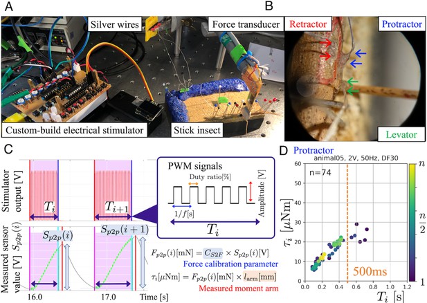
Experimental setup and joint torque calculation (A) The insect was fixed dorsal side up on a balsa wood platform.
Two small insect pins attached to the tip of the force transducer held the middle part of the femur segment of the middle leg. (B) Electrodes (arrows) implanted into the three leg muscles protractor, retractor, and levator, in the right middle leg. (C) We systematically analyzed how joint torques depended on the three PWM burst parameters amplitude [V], frequency [Hz], and duty ratio [%], and identified the combinations that most effectively and repeatedly produced torque. The upper graph shows the profile of an electrical stimulation signal for each muscle. The lower graph shows the profile of the sensor value measured with the force transducer. (D). The panel shows the calculated ThC-joint torque profile versus the burst duration during the protractor stimulations (animal05, ). In this experiment, the burst duration was varied at random, and the torque was calculated from force measurements with calibrated conversion factor and moment arm (see (C)). The voltage, frequency, and duty ratio of the PWM signals were 2.0 V, 50 Hz, and 30%, respectively. The color of the dots represents the number of stimulations (blue–yellow: 1–74). The orange dotted vertical line indicates at 500ms.
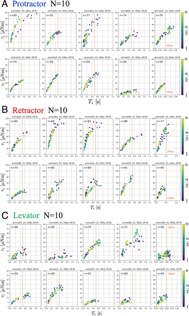
Joint torques as a function of burst duration.
Data from 10 animals with three muscles, each: (A) protractor, (B) retractor, and (C) levator muscle stimulation. The PWM burst parameters were 2.0 V. 50 Hz, and 30% duty ratio. gives the number of stimulations for each animal. Electrical stimulations were performed manually and randomly; therefore, the total number of stimuli was different for each animal. The color of the symbols indicates the order of the stimulations: blue (1) to yellow (). The positive values of joint torque represent intended (A) forward, (B) backward and (C) upward rotation of the coxa relative to the thorax. Source code and data are available on Dryad (Figure2.zip, https://doi.org/10.5061/dryad.wpzgmsbsw).
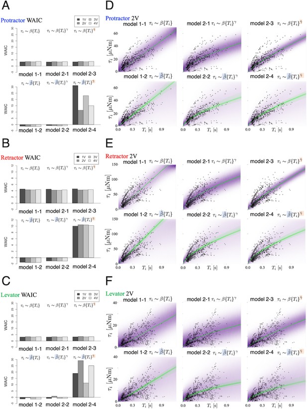
Model comparison underscores significance of inter-individual variation of slope.
We compared the six models that were explained in the ‘Model’ subsection. (A), (B), and (C) show plots of the WAIC (Watanabe, 2018) values for the protractor, retractor, and levator stimulations, respectively ( animals per muscle). The parameters with tilde, and , indicate that the parameters include inter-individual variation. PWM parameters were set as follows: (1.0 V, 2.0 V, 3.0 V, and 4.0 V), at 50 Hz and 30% duty ratio. Negative values were obtained for models 1–2 and 2–2 for all voltages and all muscles. The lowest WAIC indicates the best prediction model, as explained in the "WAIC" subsection. Right panels show Bayesian predictive estimation for the protractor (D), retractor (E), and levator (F) stimulation experiments with PWM parameters 2.0 V, 50 Hz, and 30% duty ratio. The differences in the point styles indicate individual animals. In each panel, the violet shading indicates the probability density of the distribution predictive. The green lines represent twenty samples from the posterior distribution in decreasing order of probability density. Source code and data are available on Dryad (Figure3-5.zip, https://doi.org/10.5061/dryad.wpzgmsbsw).

Predictive distributions from the linear hierarchical model (1-2) for each individual: The protractor (A), retractor (B), and levator (C) stimulation experiments with PWM parameters, 2.0 V, 50 Hz, and 30% duty ratio.
gives the number of stimulations for each animal. The color legend indicates the order of the stimulations: blue (1) to yellow (). In each panel, the violet shading indicates the probability density of the predictive distribution. The green lines represent twenty samples from the posterior distribution in decreasing order of probability density. The results demonstrate that the linear hierarchical model had an accurate predictive distribution in the range up to 500ms. Source code and data are available on Dryad (Figure3-5.zip, https://doi.org/10.5061/dryad.wpzgmsbsw).
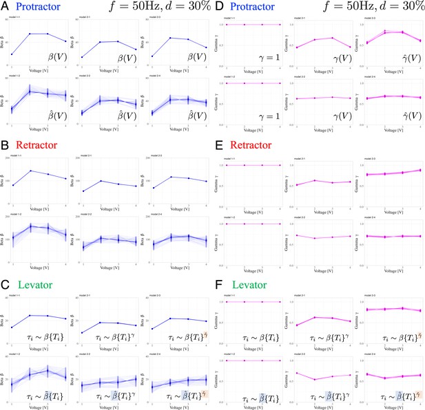
Dependence of muscle property parameters on the applied voltage and individual animals in the six models: The left graphs (A), (B), and (C) represent the estimation for for the applied voltage varied from 1.0 to 4.0 V for the six models.
(A) and (D), (B) and (E), and (C) and (F) illustrate the protractor, retractor, and levator stimulations, respectively. In (A) to (C), the upper and lower panels show non-hierarchical (1-1, 2-1, 2-3) and hierarchical (1-2, 2-2, 2-4) models for , respectively. The right graphs (D), (E), and (F) represent the estimation for in applied voltage changes. In (D) to (F), the left panel shows linear models (, 1–1, 1–2); the middle and right panels illustrate non-hierarchical (2-1, 2-2), and hierarchical (2-3, 2-4) models for , respectively. For hierarchical models (1-2, 2-2, 2-3, 2-4), the plot includes thirty samples from the posterior distribution in decreasing order of probability density, showing inter-individual variation. Source code and data are available on Dryad (Figure3-5.zip, https://doi.org/10.5061/dryad.wpzgmsbsw).

Dependence of muscle property parameters on the applied frequency of the PWM signals (2.0 V and 30% duty ratio) for the six models.
The left graphs (A), (B), and (C) present the value of estimated for an applied frequency ranging from 50 to 110 Hz for the six models. (A) and (D), (B) and (E), and (C) and (F) illustrate the protractor, retractor, and levator stimulations, respectively. In (A) to (C), the upper and lower panels refer to the non-hierarchical (1-1, 2-1, 2-3) and hierarchical (1-2, 2-2, 2-4) models for, respectively. The right graphs (D), (E), and (F) present the value of estimated for the applied voltage changes. In (D) to (F), the left panel refers to the linear models (, 1–1, 1–2), and the middle and right panels refer to the non-hierarchical models (2-1, 2-2) and hierarchical (2-3, 2-4) models for, respectively. Source code and data are available on Dryad (Figure6-7.zip, https://doi.org/10.5061/dryad.wpzgmsbsw).

Dependence of muscle property parameters on the applied duty ratio of the PWM signals (2.0 V and 50 Hz) in the six models.
The left graphs (A), (B), and (C) present the estimation for with the applied duty ratio varied from 10 to 30% for the six models. (A) and (D), (B) and (E), and (C) and (F) illustrate the protractor, retractor, and levator stimulations, respectively. In (A) to (C), the upper and lower panels present the non-hierarchical (1-1, 2-1, 2-3) and hierarchical (1-2, 2-2, 2-4) models for , respectively. The right graphs (D), (E), and (F) present the estimation for under the applied voltage changes. In (D) to (F), the left panel shows linear models (, 1–1, 1–2), and the middle and right panels illustrate the non-hierarchical (2-1, 2-2) and hierarchical (2-3, 2-4) models for , respectively. Source code and data are available on Dryad (Figure6-7.zip, https://doi.org/10.5061/dryad.wpzgmsbsw).
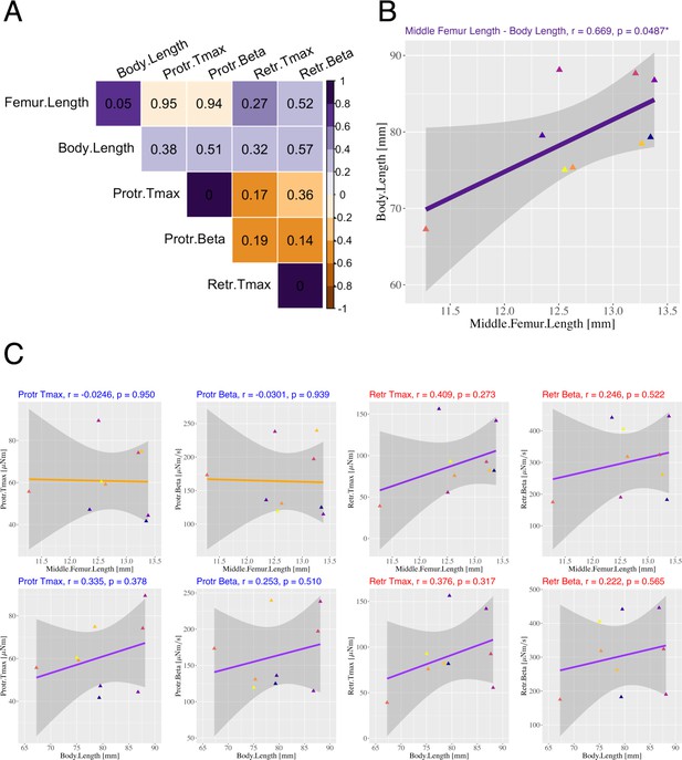
Relationship between generated joint torque and body morphology.
(A) Correlation coefficients (color: purple = 1 to orange=-1) and -values (numbers in the panel) between middle femur length, body length, Tmax, and the averaged for protractor and retractor muscles. (B) Linear regression between middle femur length and body length. The purple line represents the linear regression line. (C) Linear regression between middle femur length (upper)/body length (lower) and and for protractor (left) and retractor (right) muscles, respectively. For (B) and (C), color differences in plot points indicate individual differences (), and the gray area represents the 95% confidence interval. The correlation coefficient and -value are indicated in each panel. These data are for future follow-up studies and cannot be disclosed.
Tables
List of Stick insects used in the stimulation experiments for each muscle.
Animal ** denotes the identification number of the stick insects. We analyzed 20 animal data from ‘Animal 01’ to ‘Animal 22’ except for ‘12’ and ‘16’. Due to experimental failures and time limitations, we could not obtain stimulation data for all three muscles from the same animal on the same day. Therefore, we conducted experiments to collect data for ten animals () for each muscle through experiments using 20 animals.
| Date | Protractor | 1,2,3,4 V | Retractor | 1,2,3,4 V | Levator | 1,2,3,4 V |
|---|---|---|---|---|---|---|
| 2018.8.21. | Animal 01 | 50,49,60,50 | Animal 01 | 60,65,55,72 | ||
| 2018.8.22. | Animal 02 | 49,55,51,40 | Animal 02 | 55,68,58,65 | Animal 02 | 37,68,67,70 |
| 2018.8.27. | Animal 03 | 60,77,91,72 | Animal 03 | 94,81,63,75 | ||
| 2018.8.28. | Animal 04 | 74,69,80,77 | ||||
| 2018.8.30. | Animal 05 | 67,74,79,79 | ||||
| 2018.8.31. | Animal 06 | 75,86,76,76 | ||||
| 2018.9.03. | Animal 07 | 81,79,74,78 | Animal 07 | 82,77,81,75 | Animal 07 | 75,75,75,75 |
| 2018.9.04. | Animal 08 | 75,75,79,75 | Animal 08 | 75,71,77,84 | ||
| 2018.9.05. | Animal 10 | 74,74,74,75 | Animal 09 | 75,95,75,75 | ||
| 2018.9.19. | Animal 13 | 62,60,70,69 | Animal 11 | 50,50,50,50 | ||
| 2018.9.20. | Animal 14 | 59,59,60,59 | Animal 14 | 60,60,60,60 | ||
| 2018.9.21. | Animal 15 | 59,59,59,59 | Animal 15 | 61,60,60,51 | ||
| 2018.9.23. | Animal 17 | 59,59,60,69 | Animal 17 | 59,61,60,61 | ||
| 2018.9.24. | Animal 19 | 61,61,61,60 | Animal 18 | 60,60,59,66 | ||
| 2018.9.25. | Animal 20 | 62,60,70,60 | ||||
| 2018.9.26. | Animal 21 | 59,59,60,59 | Animal 22 | 60,60,60,60 | ||
| Total | N=10 | N=10 | N=10 |


