Collaborative hunting in artificial agents with deep reinforcement learning
- Graduate School of Informatics, Nagoya University, Japan
- Institute for Advanced Research, Nagoya University, Japan
- Graduate School of Science, Nagoya University, Japan
- Institute of Innovation for Future Society, Nagoya University, Japan
- RIKEN Center for Advanced Intelligence Project, Japan
- PRESTO, Japan Science and Technology Agency, Japan
Figures
Figure 1 with 2 supplements

Agent architecture and examples of movement trajectories.
(a) An agent’s policy is represented by a deep neural network (see Methods). A state of the environment is given as input to the network. An action is sampled from the network’s output, and the agent receives a reward and a subsequent state. The agent learns to select actions that maximize cumulative future rewards. In this study, each agent learned its policy network independently, that is, each agent treats the other agents as part of the environment. This illustration shows a case with three predators. (b) The movement trajectories are examples of interactions between predator(s) (dark blue, blue, and light blue) and prey (red) that overlay 10 episodes in each experimental condition. The experimental conditions were set as the number of predators (one, two, or three), relative mobility (fast, equal, or slow), and reward sharing (individual or shared), based on ecological findings.
Figure 1—figure supplement 1

Network architecture.
The neural network is composed of four layers. The input to the neural network was the state and the output was each possible action, namely, a total of 13 action of the ‘acceleration’ in 12 directions every 30 degrees in the relative coordinate system and ‘do nothing.’ After the first two hidden layers of the MLP with 64 units, the network branches off into two streams. Each branch has one MLP layer with 32 hidden units. Rectified linear unit (ReLU) was used as the activation function for each layer. In the visualization of the agents’ internal representations, the 32-dimensional hidden vector (parts filled in gray) was embedded in two dimensions, using t-distributed stochastic neighbor embedding (t-SNE).
Figure 1—figure supplement 2
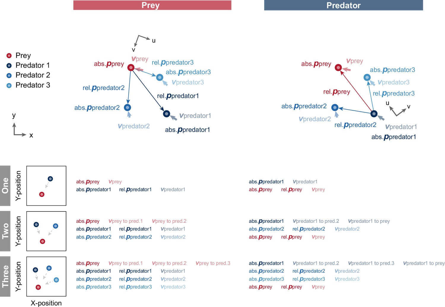
Diagram of model input.
We used position and velocity information as the state (model input) for each agent. Assuming subjective observation, each variable, except absolute position, was converted to a relative coordinate system to the opponent; namely, prey for predators and nearest predator for prey, and inputted to the model. Moreover, for the prey input in the three-predator condition, the predator indices were sorted according to the distance between the prey and each predator. Specifically, we considered predator 1, predator 2, and predator 3 descending order in terms of distance. Similarly, in the predator input in the three-predator condition, we set itself as predator 1, the closer predator to itself as predator 2, and the farther predator as predator 3. In the figure, abs., rel.,bold p, and bold v denote an absolute, relative, position, and velocity, respectively.
Figure 2 with 4 supplements
Emergence of collaborations among predators.
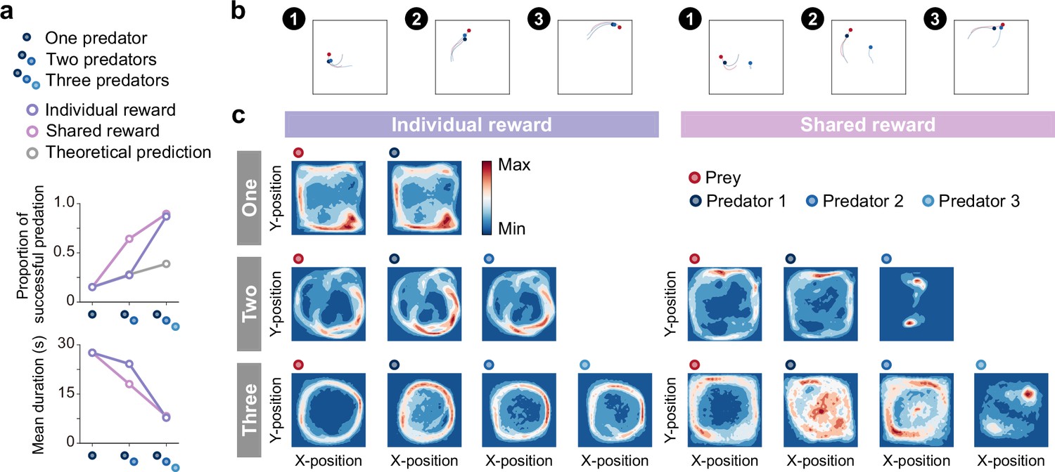
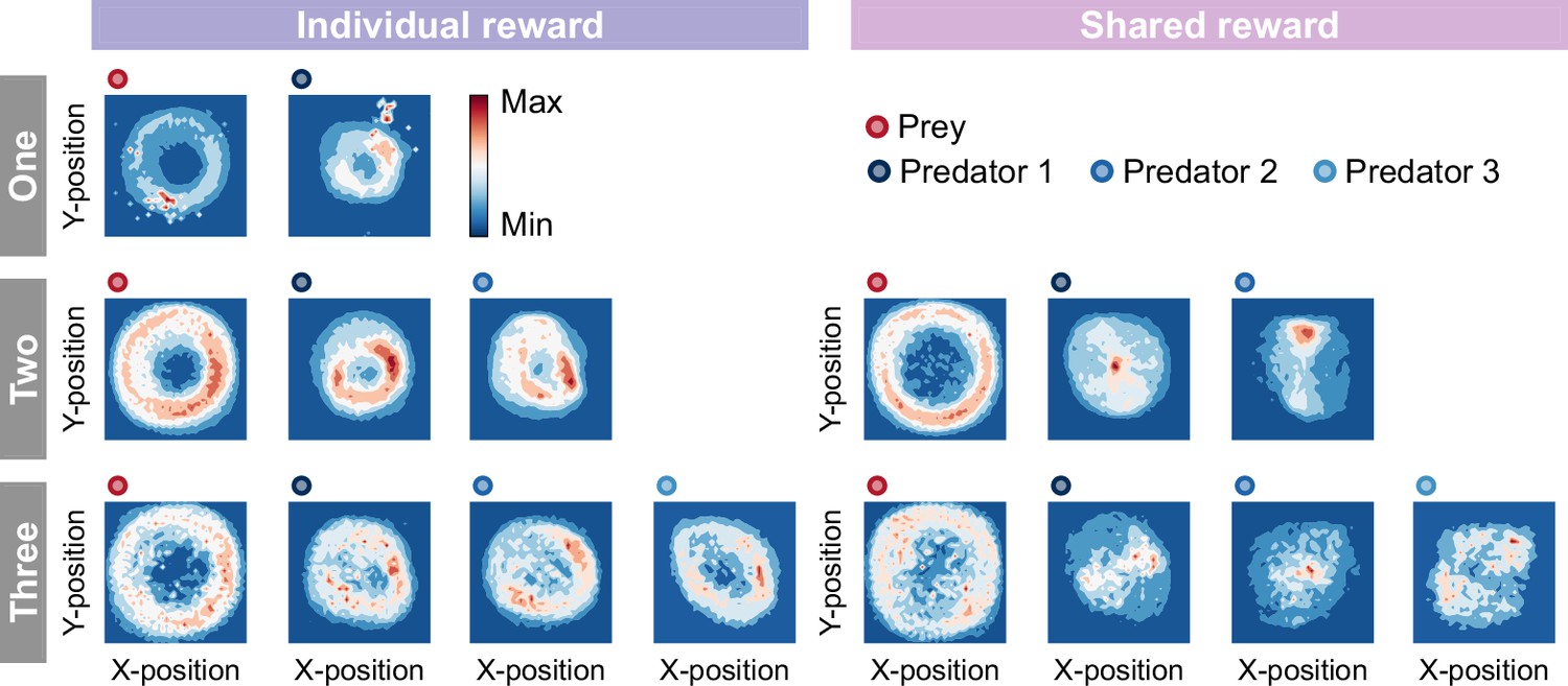
(a) Proportion of predations that were successful (top) and mean episode duration (bottom). For both panels, quantitative data denote the mean of 100 episodes ± SEM across 10 random seeds. The error bars are barely visible because the variation is negligible. The theoretical prediction values were calculated based on the proportion of solitary hunts (see Methods). The proportion of predations that were successful increased as the number of predators increased ( = 1346.67, <0.001; = 0.87; one vs. two: = 20.38, <0.001; two vs. three: = 38.27, <0.001). The mean duration decreased with increasing number of predators ( = 1564.01, <0.001; = 0.94; one vs. two: = 15.98, <0.001; two vs. three: = 40.65, <0.001). (b) Typical example of different predator routes between the individual (left) and shared (right) conditions, in the two-predator condition. The numbers (1–3) show a series of state transitions (every second) starting from the same initial position. Each panel shows the agent positions and the trajectories leading up to that state. In these instances, the predators ultimately failed to capture the prey within the time limit (30 s) under the individual condition, whereas the predators successfully captured the prey in only 3 s under the shared condition. (c) Comparison of heat maps between individual (left) and shared (right) reward conditions. The heat maps of each agent were constructed based on the frequency of stay in each position, which was cumulative for 1000 episodes (100 episodes × 10 random seeds). In the individual condition, there were relatively high correlations between the heat maps of the prey and each predator, regardless of the number of predators (One:=0.95,<0.001, Two:=0.83,<0.001 in predator 1,=0.78,<0.001 in predator 2, Three:=0.41,<0.001 in predator 1,=0.56,<0.001 in predator 2,=0.45,<0.001 in predator 3). In contrast, in the shared condition, only one predator had a relatively high correlation, whereas the others had low correlations (Two:=0.65,<0.001 in predator 1,=0.01,=0.80 in predator 2, Three:=0.17,<0.001 in predator 1,=0.54,<0.001 in predator 2,=0.03,=0.23 in predator 3).
Figure 2—figure supplement 1
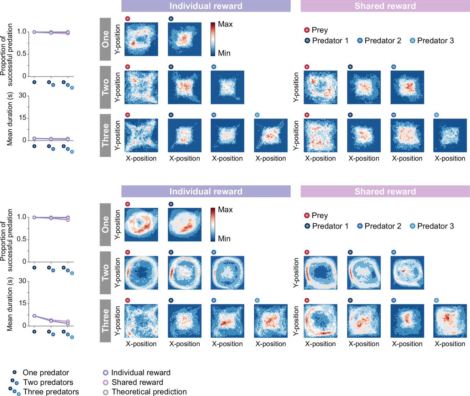
Proportion of predations that were successful, mean episode duration, and heat maps for each condition.
For both panels, quantitative data denote the mean of 100 episodes ± SEM across 10 random seeds.The theoretical prediction values were calculated based on the proportion of solitary hunts (see Methods). The heatmap of each agent was constructed based on the frequency of stay in each position, which was cumulative for 1,000episodes (100 episodes × 10 random seeds).
Figure 2—figure supplement 2
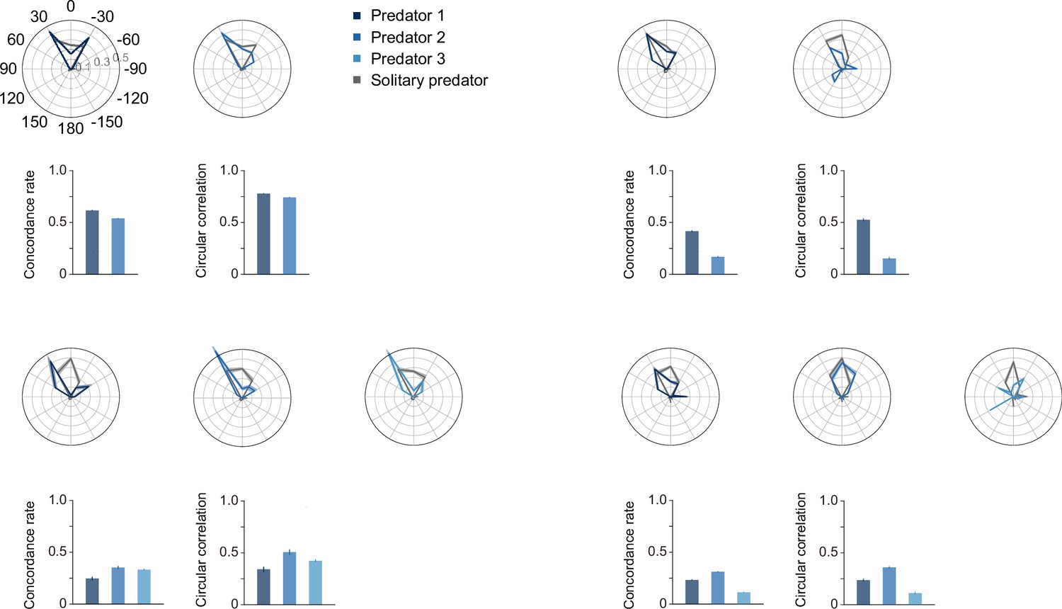
Circular histogram, concordance rate, and circular correlation.
To visualize theassociation between each predator in the two- and three-predator conditions and the baseline, which is the predatorin the one-predator condition, we produced overlays of the frequency of selection for each action. We calculated concordance rates and circular correlations to quantitatively evaluate these associations of action selection. The concordance rate has the advantage of being able to compare all 13 actions, whereas the circular correlation has theadvantage of being able to consider the proximity among each action, although it can only evaluate 12 actions,excluding ‘do nothing.’ As shown in this figure, the two indices showed similar trends. The predators whose heat maps were similar to that of their prey tended to have higher values on these indices. For all panels, quantitative datadenote the mean of 100 episodes ± SEM across 10 random seeds.
Figure 2—figure supplement 3

Scaled distance among predators and proportion of prey capture.
Scaled distance is ameasure of how far a predator moves to capture its prey compared with the other predators during a hunt. Although simplified, this distribution reflects the role each predator played in a hunt. Specifically, if there is a large difference in the scaled distance among predators, individuals with a larger scaled distance (greater than 1) could play the role of ‘chaser’ (or ‘driver’), while individuals with a smaller scaled distance (less than 1) could play the role of ‘blocker’ (or ‘ambusher’). Moreover, if these distances do not differ among predators (concentrated near 1), it is likely that each predator pursued prey in the same manner, suggesting that there was no role division during the hunt. Furthermore, these distributions can be used to capture the flexibility of role division among predators. That is, if the distributions are separate and do not overlap, there is a division of roles among predators, and these roles are fixed inany hunt. On the other hand, if the distributions are separate but some of them overlap, the roles may have switched across hunts. Our results show that the distribution in the individual condition was concentrated around 1, whereas in the shared condition it was divided among individuals. This means that there was rarely role division among predators in the individual condition, while there was role division in the shared condition. These characteristics were more pronounced in the two-predator condition than in the three-predator condition. Perhaps this depends on the episode duration; the duration tends to be longer in the two-predator condition, and the difference in distance is likely to be clearer. Note that even under the two-predator condition, there was some overlap in the distribution inthe shared condition. This indicates that the basic roles were fixed among individuals, but interchanged according to the situation (or episode) in the condition. Additionally, because these role divisions are often discussed in the context of cooperation and cheating, we calculated the proportion of prey capture for each predator. The results did not indicate which role was more likely to catch the prey. That is, in the shared × two conditions, the chaser tended to catch more prey, but, on the other hand, in the shared × three conditions, the blocker tended to catch more prey. For all panels, quantitative data denote the mean of 100 episodes ± SEM across 10 random seeds.
Figure 2—figure supplement 4

Typical example of coordinated hunting behavior in the three × individual condition.
The numbers (1 to 3) show a series of state transitions (every 0.6 s). Each panel shows the agent positions and the trajectories leading up to that state.
Figure 3 with 11 supplements

Embedding of internal representations underlying collaborative hunting.
(a) Two-dimensional t-distributed stochastic neighbor embedding (t-SNE) embedding of the representations in the last hidden layers of the state-value stream (top) and action-value stream (bottom) in the shared reward condition. The representation is assigned by the policy network of each agent to states experienced during predator-prey interactions. The points are colored according to the state values and standard deviation of the action values, respectively, predicted by the policy network (ranging from dark red (high) to dark blue (low)). (b) Corresponding states for each number in each embedding. The number (1–5) in each embedding corresponds to a selected series of state transitions. The series of agent positions in the state transitions (every second) and, for ease of visibility, the trajectories leading up to that state are shown. (c) Embedding colored according to the distances between predators and prey in the individual (left) and shared (right) reward conditions. Distances 1 and 2 denote the distances between predator 1 and prey and predator 2 and prey, respectively. If both distances are short, the point is colored blue; if both are long, it is colored white.
Figure 3—figure supplement 1

Two-dimensional t-distributed stochastic neighbor embedding (t-SNE) embedding of the representations in the last hidden layers of the state-value stream (top) and action-value stream (bottom) in the individual reward condition, in the slow × two conditions.
The representation is assigned by the policy network of each agent to states experienced during predator-prey interactions. The points are colored according to the state values and standard deviation of the actionvalues, respectively, predicted by the policy network (ranging from dark red (high) to dark blue (low)).
Figure 3—figure supplement 2
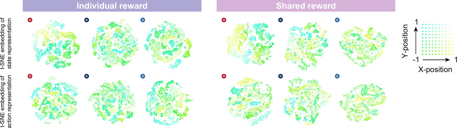
Two-dimensional t-distributed stochastic neighbor embedding (t-SNE) embedding colored according to the absolute coordinates of itself in the individual (left) and shared (right) reward conditions, in the slow × two conditions.
The absolute coordinates (i.e. x and y positions) are directly associated with the reward, as are the distances between prey and predators, because each agent receives a negative reward (-1) for leaving the play area. We, therefore, colored the internal representation of the agent according to its position. The upper left corner of the play area corresponds to cyan, the lower left to green, the upper right to white, and the lower right to yellow. The embedding of state representations in the prey seems to be roughly clustered according to absolute position, compared to those of the predators. These indicate that prey might estimate the state and action values and make decisions associated with absolute position-dependent representations compared to predators.
Figure 3—figure supplement 3
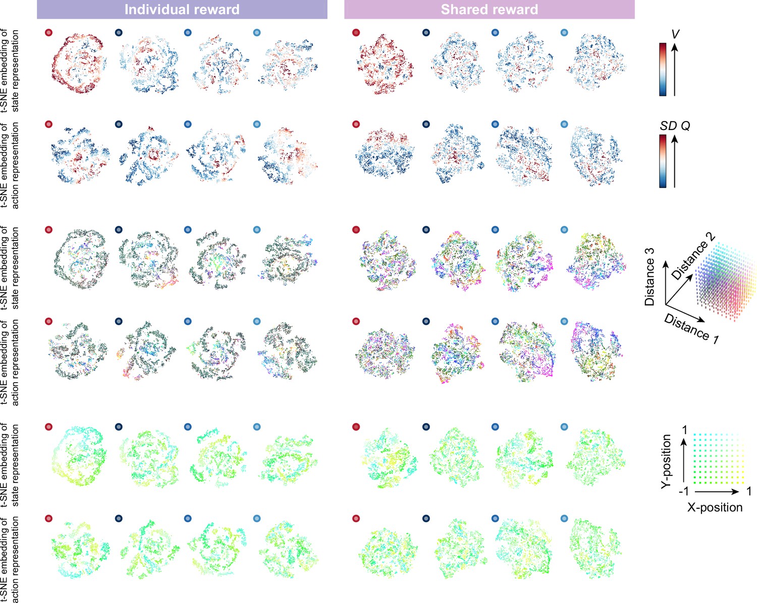
Two-dimensional t-distributed stochastic neighbor embedding (t-SNE) embedding of the representations in the last hidden layers ofstate-value stream and action-value stream, in the slow × three conditions.
The points are colored according to the state values and standard deviation of the action values predicted by the policy network (top), the distances between prey and predators (middle), and absolute coordinates of itself, respectively.
Figure 3—figure supplement 4

Corresponding state-action values (Q-values) for each state.
We show the value for eachaction of each agent in a selected series of state transitions (scenes 1 to 5). The panels on the left side of the figure are the same as the plot in Figure 3. For both predator and prey, each action is defined in terms of a relative coordinate system to the opponent. In other words, action 1 denotes movement toward the opponent (for the prey, the nearest predator) and action 7 denotes movement in the opposite direction of the opponent. Thus, in the estimated action values of the prey, actions 5 to 9 tend to show relatively high values, and in those of predators, actions 1, 2, 3, 11, and 12 tend to show relatively high values. These results suggest that proximity to rewards plays a major role in estimating state-action values.
Figure 3—figure supplement 5
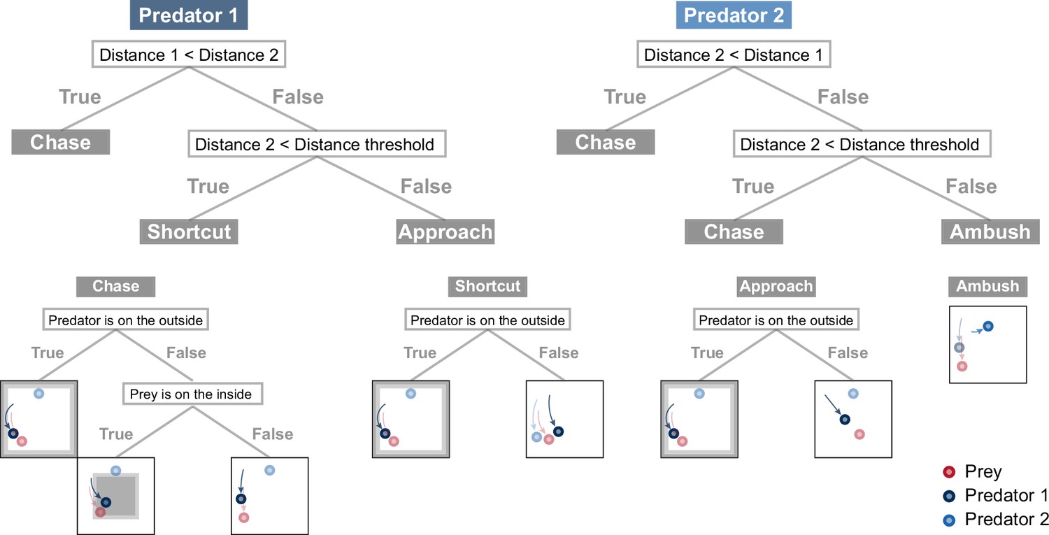
Rule-based predator agent architectures.
For consistency with the deep reinforcement learning agents, the input to the rule-based agents used to make decisions is limited to the current information (e.g. position and velocity), and the output is provided in a relative coordinate system to the prey. The predator first determines whether it, or another predator, is closer to the prey, and then, if the other predator is closer, it determines whether the distance 2 is less than the specified distance threshold. The decision rule for each predator is selected by this branching, with predator 1 adopting the three rules ‘chase,’ ‘shortcut,’ and ‘approach,’ and predator 2 adopting the two rules ‘chase’ and ‘ambush’ (see Methods for details). In the chase, the predator first determines whether it is near the outer edge of the play area and, if so, selects actions that will prevent it from leaving the play area. If the predator is not on the outside of the play area, then it determines whether the prey is on the inside of the play area,and, if so, selects actions that will drive them to the outside. In other situations, it selects actions so that the direction of movement is aligned with that of their prey. In the shortcut, the predator determines whether it is near the outeredge of the play area, and if so, selects the actions described above, otherwise selects actions that will produce shorter paths to the prey. In the approach, the predator determines whether it is near the outer edge of the play area and, if so, selects the actions described above, otherwise it selects actions that move it toward the prey. In the ambush, the predator selects actions that move toward the top center or bottom center of the play area and remain there until the situation changes.
Figure 3—figure supplement 6
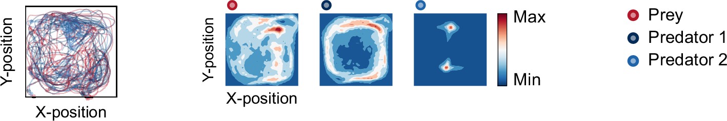
Movement trajectories (left) and heat maps (right) of the rule-based predator agents.
The movement trajectories are examples of predator(s) (dark blue and blue) and prey (red) interactions that overlay 10 episodes. The proportion of successful predation and mean episode duration were 74.4 ± 0.54 and 12.9 ± 0.12 (mean of 100 episodes ± SEM across 10 random seeds), respectively. The heat map of each agent was constructed based on the frequency of stay in each position, which is cumulative for 1,000 episodes (100 episodes × 10 random seeds). One predator had a relatively high correlation between the heat maps, whereas the others had a lowcorrelation (r = 0.60, p<0.001 in predator 1, r = 0.20, p<0.001 in predator 2). This trend in results is similar to that in the deep reinforcement learning predator agents (compare Figure 2c). Note that, in the rule-based agentsimulation, the prey’s decision was made by a policy network in the two × shared condition (i.e. predatorrule-based agent vs. prey deep reinforcement learning agent).
Figure 3—figure supplement 7

Two-dimensional t-distributed stochastic neighbor embedding (t-SNE) embedding of the representations in the last hidden layers ofthe linear network (top) and the nonlinear network (bottom) in behavioral cloning.
The embedding is colored according to the distances between predators and prey. Distances 1 and 2 denote the distance between predator 1 and prey and predator 2 and prey, respectively. If both distances are short, the point is colored blue; if both are long, it is colored white. Note that the accuracy in behavioral cloning from the top 1 to the top 5 was, in ascending order, 0.47, 0.61, 0.71, 0.78, 0.80 for predator 1 and 0.44, 0.55, 0.60, 0.66, and 0.70 for predator 2 for the linear network, and 0.65, 0.77, 0.82, 0.88, and 0.95 for predator 1 and 0.68, 0.78, 0.82, 0.85, and 0.90 for predator 2 for the nonlinear network.
Figure 3—figure supplement 8
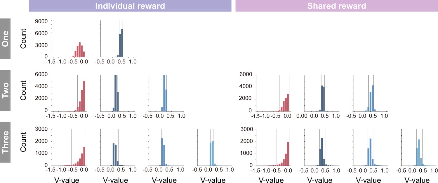
Histogram of the state value (V-value) in the individual (left) and shared (right) conditions.
In coloring the embedding, the lower and upper limits of coloring were set to the fifth percentile and 95th percentile (gray lines), respectively, to prevent visibility from being compromised by extreme values that rarely occur.
Figure 3—figure supplement 9
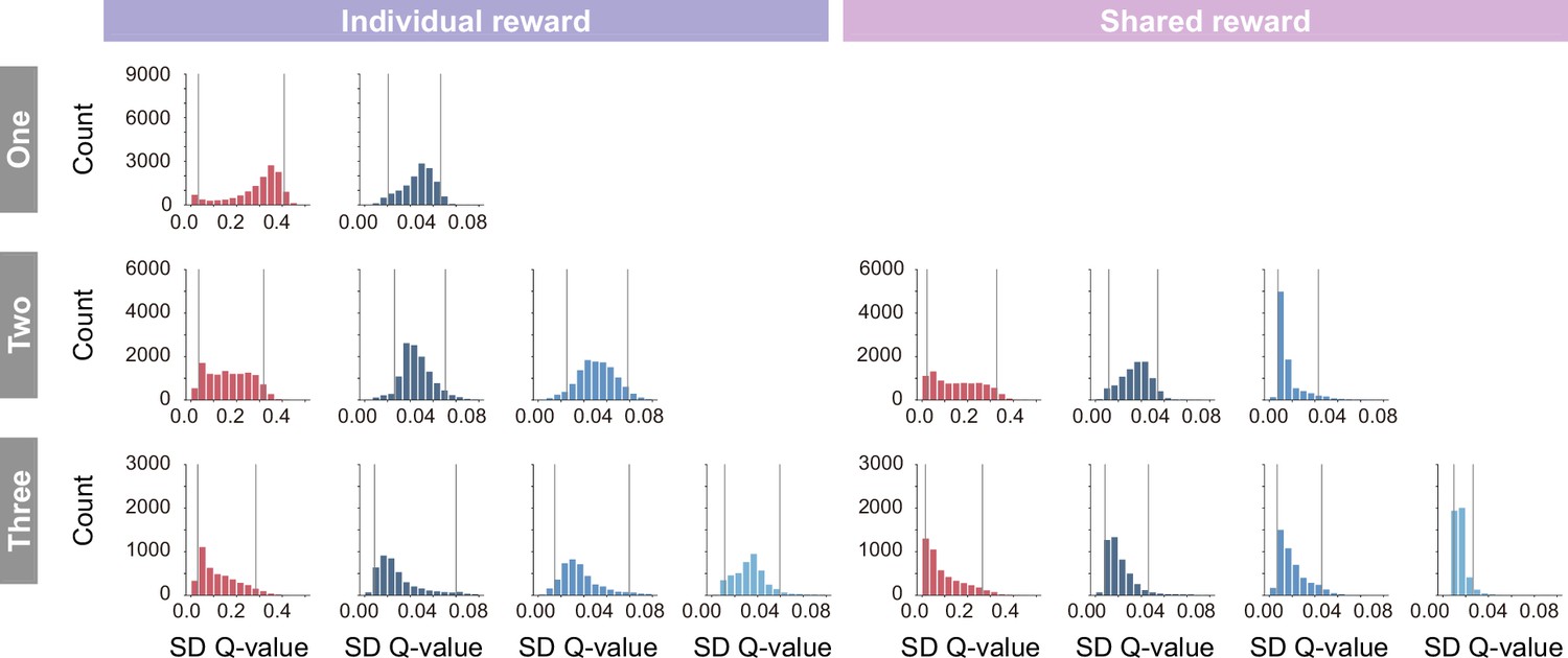
Histogram of the standard deviation of state-action values (Q-values) in individual (left) and shared (right) conditions.
In coloring the embedding, the lower and upper limits of coloring were set to the fifth percentile and 95th percentile (gray lines), respectively, to prevent visibility from being compromised by extreme values that rarely occur.
Figure 3—figure supplement 10
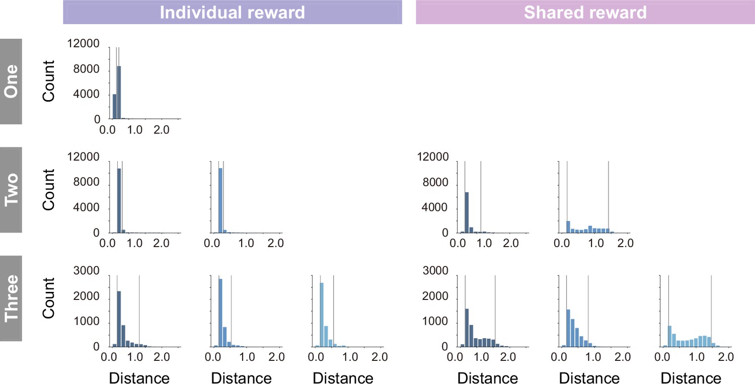
Histogram of the distance between the prey and each predator in individual (left) and shared (right) conditions.
In coloring the embedding, the lower and upper limits of coloring were set to the fifth percentile and 95th percentile (gray lines), respectively, to prevent visibility from being compromised by extreme values that rarely occur.
Figure 3—figure supplement 11
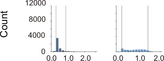
Histogram of the distance between the prey and each predator in the simulations, using rule-based predator agents.
In coloring the embedding in behavioral cloning, the lower and upper limits of coloring were set to the fifth percentile and 95th percentile (gray lines), respectively, to prevent visibility from being compromised by extreme values that rarely occur.
Figure 4 with 2 supplements

Superior performance of predator agents for prey controlled by humans and comparison of internal representations.
(a) Proportion of predations that were successful (top) and mean episode duration (bottom). For both panels, the thin line denotes the performance of each participant, and the thick line denotes the mean. The theoretical prediction values were calculated based on the mean of proportion of solitary hunts. The proportion of predations that were successful increased as the number of predators increased ( = 276.20, <0.001; = 0.90; one vs. two: = 13.80, <0.001; two vs. three: = 5.9402, <0.001). The mean duration decreased with an increasing number of predators ( = 23.77, <0.001; = 0.49; one vs. two: = 2.60, =0.029; two vs. three: = 5.44, <0.001). (b) Comparison of two-dimensional t-distributed stochastic neighbor embedding (t-SNE) embedding of the representations in the last hidden layers of state-value stream between self-play (predator agents vs. prey agent) and joint play (predator agents vs. prey human).
Figure 4—figure supplement 1

Comparison of two-dimensional t-distributed stochastic neighbor embedding (t-SNE) embedding of the internal representations.
To visualize the associations of states experienced by predator agents versus agents (self-play) and versus humans (jointplay), we show colored two-dimensional t-SNE embedding of the representations in the last hidden layer of the action-value stream. Similar to those of the state stream (Figure 4b), the experienced states were quite distinct,especially in the one- and two-predator conditions.
Figure 4—figure supplement 2
Comparison of heat maps between individual (left) and shared (right) reward conditions in joint play.
The heat map of each agent was made based on the frequency of stay in each position which iscumulative for 500 episodes (50 episodes × 10 participants). Our results showed a similar trend between self-play (predator agents vs. prey agent) and joint play (predator agents vs. prey human) in terms of role division among predators. For example, in the individual condition, the heat maps between/among predators were similar, indicating that there was no clear division of roles. On the other hand, in the shared condition, the heat maps between/among predators differed and it indicates that the roles were divided among them. In addition, one of the differences fromself-play was the instability of the predator agent’s behavior in the one-predator condition. As shown in the figure, under certain conditions, the predator agent stopped moving from its location (the upper right corner of the area).
Videos
Video 1
Example videos in the one-predator conditions.
Video 2
Example videos in the two-predator conditions.
Video 3
Example videos in the three-predator conditions.
Additional files
Download links
A two-part list of links to download the article, or parts of the article, in various formats.
Downloads (link to download the article as PDF)
Open citations (links to open the citations from this article in various online reference manager services)
Cite this article (links to download the citations from this article in formats compatible with various reference manager tools)
Collaborative hunting in artificial agents with deep reinforcement learning
eLife 13:e85694.
https://doi.org/10.7554/eLife.85694


