Figures and data in Quantitative modeling of the emergence of macroscopic grid-like representations

Figures
Tables
Additional files

6 figures, 1 table and 1 additional file

Figures

Figure 1 with 4 supplements

Download asset Open asset

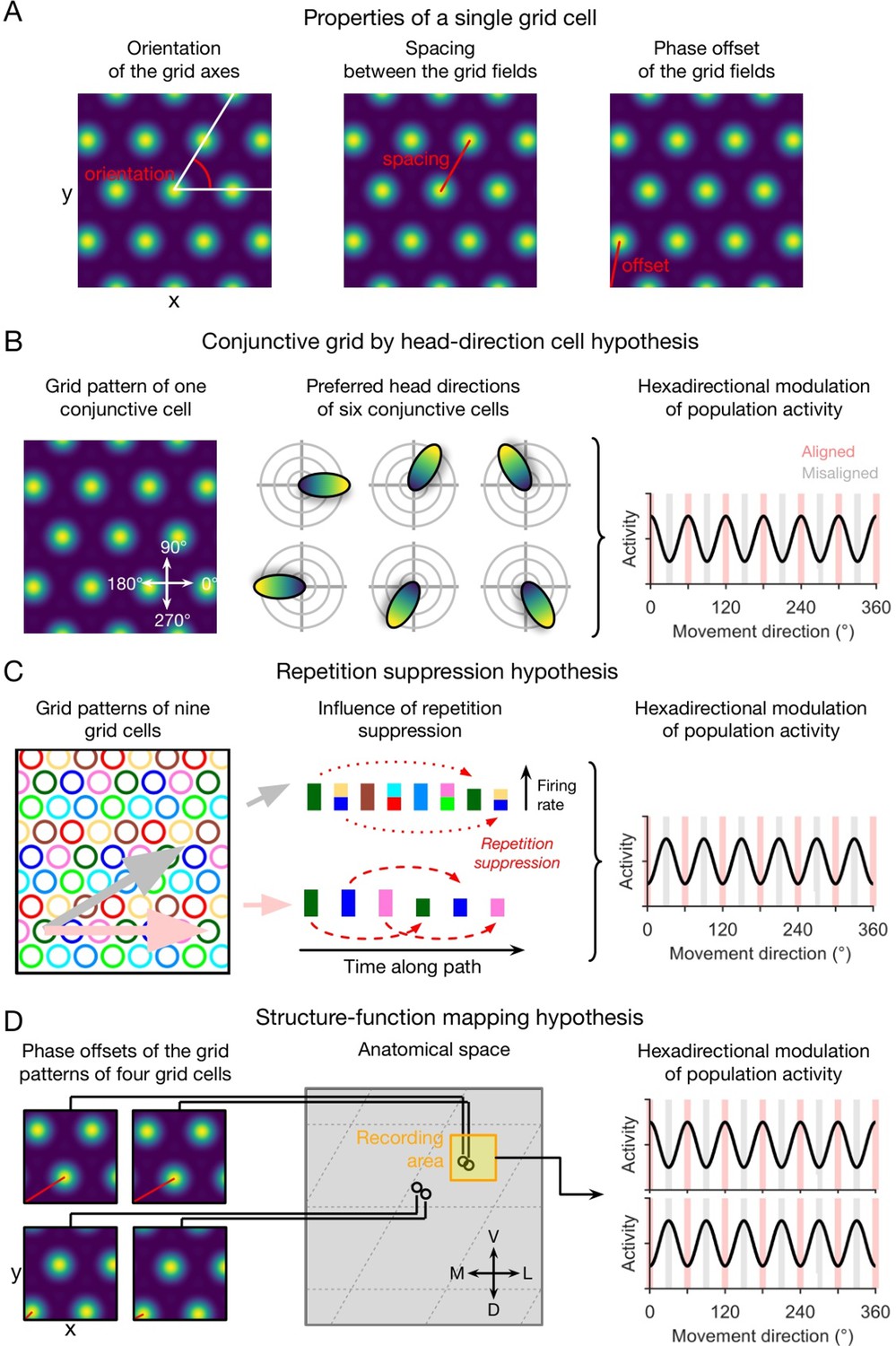
Qualitative hypotheses on the emergence of macroscopic grid-like representations in the human entorhinal cortex.

(A) Grid-cell properties comprise grid orientation, grid spacing, and grid phase offset. (B) Conjunctive grid by head-direction cell hypothesis. Macroscopic grid-like representations (right) may emerge from the firing of conjunctive grid by head-direction cells (left and middle) that exhibit increased firing when the subject moves aligned as compared to misaligned with the grid axes (right) (Doeller et al., 2010). (C) Repetition suppression hypothesis. In a grid cell population with similar grid orientations and grid spacings but with distributed phases (left; colored circles represent firing fields of different grid cells), aligned movements (horizontal pink arrow) lead to more frequent activation (shorter distance between firing fields) of a smaller number of different grid cells, whereas misaligned movements (diagonal gray arrow) lead to less frequent activation (larger distance between firing fields) of a higher number of different grid cells (Doeller et al., 2010). Thus, aligned movements may lead to more pronounced repetition suppression as compared to misaligned movements (middle), resulting in a hexadirectional modulation of population spiking activity and thus in the emergence of grid-like representations (right). (D) Structure-function mapping hypothesis. Because anatomically adjacent grid cells exhibit similar grid phase offsets (in addition to similar grid orientations and grid spacings) (Gu et al., 2018), recordings from a limited number of grid cells with a non-random distribution of phase offsets may lead to macroscopic grid-like representations. The left panel shows the grid phase offset of four different grid cells, whose anatomical locations are illustrated in the middle panel. Depending on the subject’s starting location relative to the phase offset of the grid fields, movements aligned or misaligned with the grid axes lead to higher sum grid cell activity as compared to misaligned or aligned movements (right panel). Furthermore, the orientation of hexadirectional modulation may shift when recording from neighboring voxels in anatomical space due to a shift in the clustered phase offsets. D, dorsal; L, lateral; M, medial; V, ventral. Figure 1 has been adapted from Figure 3 from Kunz et al., 2019.

Figure 1—figure supplement 1

Download asset Open asset

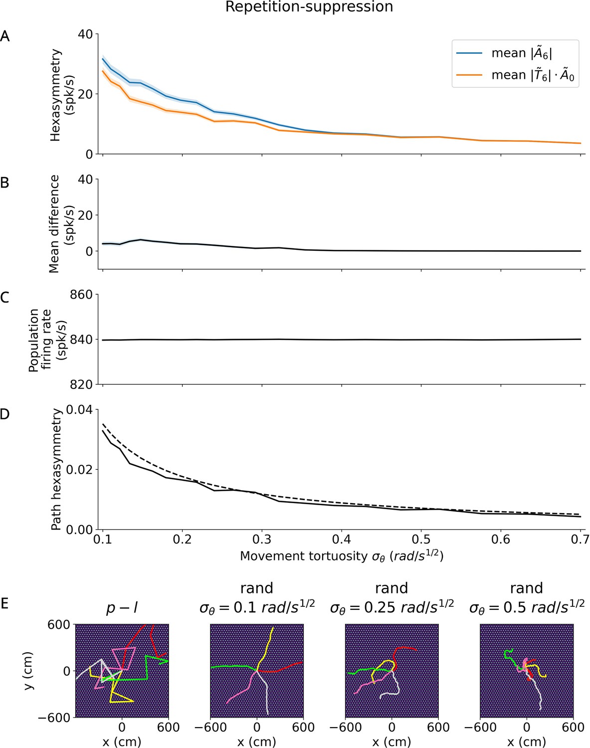
Effect of tortuosity on the hexasymmetry for the repetition suppression hypothesis with random walks ( $Δ t = 0.01 s$ s, $T = 9000 s$ , $τ_{r} = 3 s$ , $w_{r} = 1$ ).

(A) The hexasymmetry $| {\tilde{A}}_{6} |$ (blue) and the scaled path hexasymmetry $| {\tilde{T}}_{6} | \cdot {\tilde{A}}_{0}$ (orange) as a function of the movement tortuosity $σ_{θ}$ of a random walk. The shaded areas represent the standard error when averaging over 100 realizations of the trajectory, each with an initial direction sampled from a random uniform distribution on the interval $[0, 2 π)$ . (B) The mean difference between $| {\tilde{A}}_{6} |$ and $| {\tilde{T}}_{6} | \cdot {\tilde{A}}_{0}$ as a function of the movement tortuosity $σ_{θ}$ . Note that $| {\tilde{A}}_{6} | \geq | {\tilde{T}}_{6} | \cdot {\tilde{A}}_{0}$ for $σ_{θ} \leq 0.4$ . For $σ_{θ} > 0.4$ the two curves begin to overlap: repetition suppression ceases to have a significant effect and the hexasymmetry $| {\tilde{A}}_{6} |$ is primarily dictated by the path hexasymmetry. The dip in the mean difference near $σ_{θ} \sim 0.1$ is thought to be due to numerical noise. (C) The mean firing rate $\tilde{A_{0}}$ does not depend on movement tortuosity $σ_{θ}$ , indicating that any effect of repetition suppression on the population firing rate is small. (D) Path hexasymmetry $| {\tilde{T}}_{6} |$ as a function of the movement tortuosity $σ_{θ}$ . The solid line depicts the mean path hexasymmetry averaged over 100 realizations of a trajectory, while the dashed line plots the analytical result in Equation 65. (E) Leftmost panel: Five examples (colored line segments) of a piecewise linear (‘p-l’) trajectory; each linear path segment has a length of 300 cm. Three rightmost panels: Five example random-walk (‘rand’) trajectories (colored curves) for three different values of the movement tortuosity $σ_{θ}$ with total simulation time $T = 60$ s and a total path length of 600 cm. For illustration purposes, the initial directions of example random-walk trajectories were chosen such that they are regularly distributed on the interval $[0, 2 π)$ . When viewed on a scale within the range of ±600 cm, increasing the tortuosity from 0.1 to 0.5 results in increasingly more curved trajectories. The bright dots in all panels of (E) show the grid fields with grid spacing 30 cm, which is small when viewed on this scale. In the simulations for Figures 2—5, the random-walk trajectories have total lengths of 90,000 cm or longer and use a movement tortuosity of $σ_{θ} = 0.5 {rad/s}^{1 / 2}$ .

Figure 1—figure supplement 2

Download asset Open asset

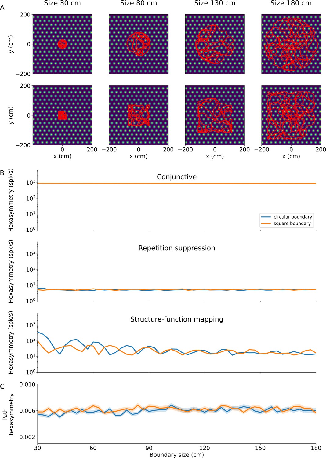
Effect of size and shape of finite environments on hexasymmetry.

(A) Examples of bounded random-walk trajectories ( $Δ t = 0.01$ s, $T = 9000$ s, $v = 10$ cm/s, $σ_{θ} = 0.5$ rad/s^1/2; see Section ‘Environments with boundaries’ for details on the generation of bounded trajectories) within square boundaries (bottom) or circular boundaries (top) of varying sizes increasing from left to right (numbers at top labeled by ‘size’ indicate ‘half of side length’ for square boundaries or ‘radius’ for circular boundaries). Trajectories are overlaid on the firing field of an example grid cell. The lengths of the depicted trajectories are modified for illustration purposes, and do not reflect the full extent of trajectories used to calculate hexasymmetries. (B) Hexasymmetry for the three hypotheses for different sizes of the boundaries; blue, circular boundary; orange, square boundary. For all three hypotheses, the ‘ideal’ parameter sets were used; for values of the parameters, see Table 1. For the conjunctive grid by head-direction hypothesis and the repetition suppression hypothesis, the obtained values of the hexasymmetry have a weak (if any) dependence on boundary shape and size (apart from fluctuations due to noise in different realizations), and the obtained values are similar in magnitude to those obtained in infinite environments: Figure 2F for ‘conjunctive’, Figure 3E for ‘repetition suppression’. In the case of the structure-function mapping hypothesis, the strong clustering of grid phase offsets combined with the tendency of the simulated agent to move along the walls of the boundary results in a dependence of the hexasymmetry on the environment size. This effect is largest for smaller environment sizes. As the size of the environment is increased, the agent more uniformly samples the space, and the hexasymmetry approaches the magnitude of that obtained in infinite environments (Figure 4C). (C) Path hexasymmetry for different sizes of the boundaries. In (B) and (C), lines represent the mean and shaded areas represent the standard error as obtained from 50 trajectories.

Figure 1—figure supplement 3

Download asset Open asset

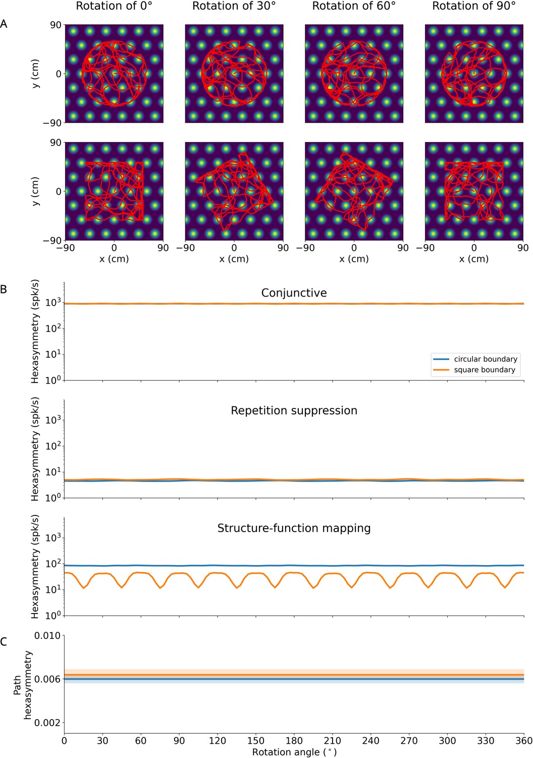
Effect of rotation of finite environments on hexasymmetry.

(A) Examples of bounded random-walk trajectories ( $Δ t = 0.01$ s, $T = 9000$ s, $v = 10$ cm/s, $σ_{θ} = 0.5$ rad/s^1/2; see Section ‘Environments with boundaries’ for details on the generation of bounded trajectories) within circular (top) or square (bottom) boundaries for different rotation angles (numbers at top) relative to the grid orientation. Trajectories are overlaid on the firing field of an example grid cell. The lengths of the depicted trajectories are modified for illustration purposes, and do not reflect the full extent of trajectories used to calculate hexasymmetries. (B) Hexasymmetry for the three hypotheses for different rotation angles of the trajectory; blue: circular boundary; orange: square boundary. For the conjunctive grid by head-direction hypothesis and the repetition suppression hypothesis, the obtained values of the hexasymmetry have a weak (if any) dependence on boundary shape and orientation (apart from fluctuations due to noise in different realizations), and the obtained values are similar in magnitude to those obtained in infinite environments: Figure 2F for ‘conjunctive’, Figure 3E for ‘repetition suppression’. In the case of the structure-function mapping hypothesis, the strong clustering of grid phase offsets combined with the tendency of the simulated agent to move along the walls of the boundary results in a periodic dependence on the boundary orientation in square environments when the sides of the square align with the strongly clustered grid firing fields. For all three hypotheses, the ‘ideal’ parameter sets were used; for values of the parameters, see Table 1. (C) Path hexasymmetry does not depend on the rotation angle of the trajectory. In (B) and (C), lines represent the mean and shaded areas represent the standard error as obtained from 50 random-walk trajectories with the same parameters as in Table 1.

Figure 1—figure supplement 4

Download asset Open asset

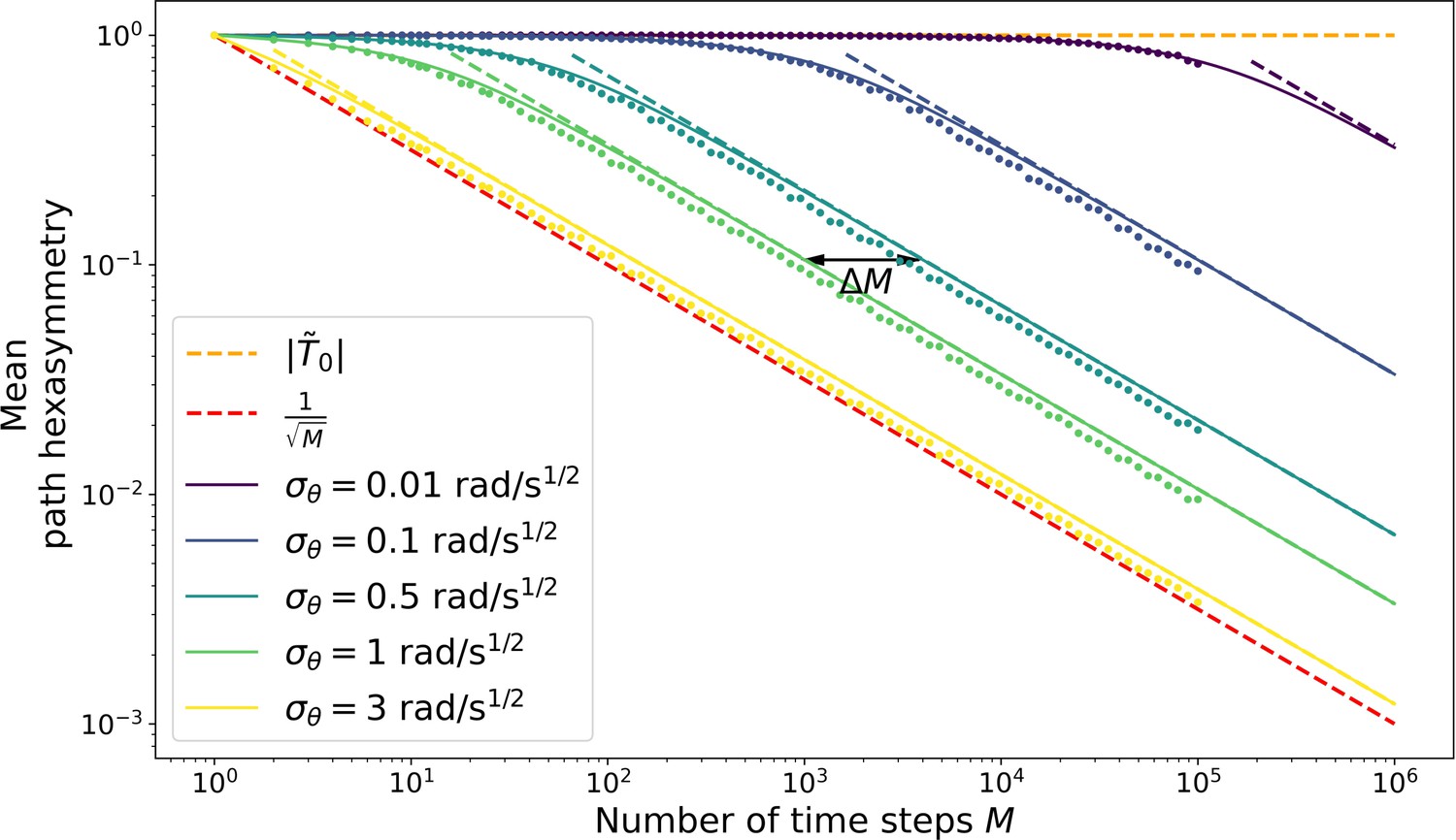
Hexasymmetry of random-walk trajectories.

The (horizontal) orange dashed line shows the offset (or maximum) of the path hexasymmetry, ${\tilde{T}}_{0} \equiv 1$ . The (diagonal) red dashed line shows the average path hexasymmetry $| {\tilde{T}}_{6} | = 1 / \sqrt{M}$ associated with randomly sampling a movement direction at each time step from a uniform distribution on the interval $[0, 2 π)$ . Solid colored curves show an upper bound for the mean path hexasymmetry of a random walk as a function of the number of time steps (square root of Equation 57) for five different movement tortuosities $σ_{θ}$ and a simulation time step size $Δ t = 10$ ms. The corresponding five colored dashed lines show an approximation ( $| {\tilde{T}}_{6} | \propto 1 / \sqrt{M}$ , Equation 65) to the solid curves; the approximation is excellent if the number $M$ of time steps is large enough. Colored dots show the respective mean path hexasymmetries obtained from numerical simulations (Equation 1). The black arrow shows the multiplicatory shift in the number of time steps that is necessary to obtain the same hexasymmetry for a trajectory with $σ_{θ} = 0.5 {rad/s}^{1 / 2}$ as for a trajectory with $σ_{θ} = 1 {rad/s}^{1 / 2}$ , as derived in Equation 70.

Figure 2 with 2 supplements

Download asset Open asset

Conjunctive grid by head-direction (HD) cell hypothesis.

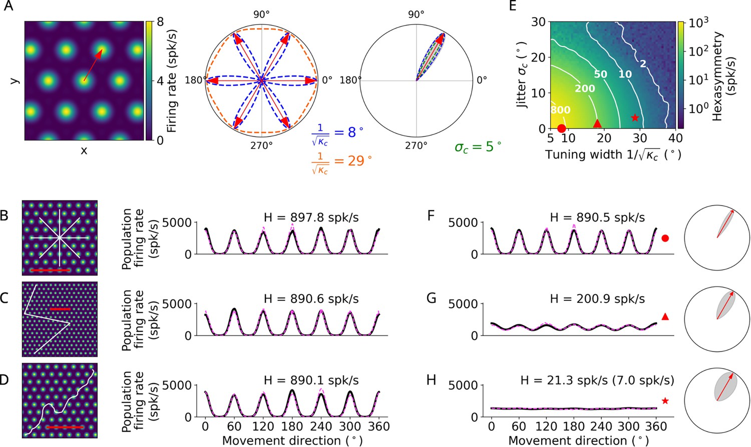
(A) Left: The preferred head direction (red arrow) of a single conjunctive cell is aligned to one of the grid axes (Doeller et al., 2010). Two factors add noise to this relation: the HD tuning has a certain width ( $1 / \sqrt{κ_{c}}$ ) and the alignment of grid orientation to HD tuning angle is jittered ( $σ_{c}$ ). Middle: Distribution of the tuning width $1 / \sqrt{κ_{c}}$ around all possible grid axes for two example values. Right: Convolution (gray) between the distributions of the jitter $σ_{c} = 5^{\circ}$ and tuning width $1 / \sqrt{κ_{c}} \approx {8.1}^{\circ}$ ( $κ_{c} = 50 {rad}^{- 2}$ ) to obtain the effective HD tuning of a single conjunctive cell around one grid axis. (**B–D**) Simulation of the conjunctive hypothesis using ‘ideal’ parameters of $κ_{c} = 50 {rad}^{- 2}$ and $σ_{c} = 0^{\circ}$ . The scale bars (red) represent a distance of 120 cm. (B) Left: Illustration of a star-like walk (path segments are cut for illustration purposes), overlaid onto the firing pattern of a single grid cell. Right: Population firing rate as a function of the subject’s movement direction (which is identical with heading direction in our simulations) for star-like runs with mean firing rate ${\tilde{A}}_{0} = 1279.7$ spk/s (for 1024 cells) and path hexasymmetry $| {\tilde{T}}_{6} | < 10^{- 10}$ ; see Methods for definitions of ${\tilde{A}}_{0}$ and ${\tilde{T}}_{6}$ . (C) Left: Illustration of a piecewise linear walk (cut for illustration purposes), overlaid onto the firing pattern of a single grid cell. Right: Population firing rate as a function of movement direction for piecewise linear walks with ${\tilde{A}}_{0} = 1279.3$ spk/s and $| {\tilde{T}}_{6} | < 10^{- 10}$ . (D) Left: Illustration of a random walk (cut for illustration purposes), overlaid onto the firing pattern of a single grid cell. Right: Population firing rate as a function of movement direction for random walks with ${\tilde{A}}_{0} = 1281.0$ spk/s and $| {\tilde{T}}_{6} | = 6.7 \cdot 10^{- 3}$ . (E) Hexasymmetry (color coded) as a function of HD tuning width and alignment jitter for star-like walk trajectories at an offset of $(0, 0)$ . Higher hexasymmetry values are achieved for stronger HD tuning and tighter alignment of the preferred head directions to the grid axes. The red symbols correspond to the three parameter combinations used in subplots (**B–D**) and (**F–H**) for further illustration. Large tuning widths ( $κ_{c} \to 0$ ) correspond to cosine tuning for which the hexasymmetry approaches 0. (F) Population firing rate as a function of movement direction for a random-walk trajectory with jitter $σ_{c} = 0$ and concentration parameter $κ_{c} = 50 {rad}^{- 2}$ (tuning width $\approx {8.1}^{\circ}$ ). (G) Population firing rate as a function of movement direction for a random walk with jitter $σ_{c} = {1.5}^{\circ}$ and concentration parameter $κ_{c} = 10 {rad}^{- 2}$ (tuning width $\approx {18.1}^{\circ}$ ). (H) Population firing rate as a function of movement direction for a random walk with jitter $σ_{c} = 3^{\circ}$ and concentration parameter $κ_{c} = 4 {rad}^{- 2}$ (tuning width $\approx {28.6}^{\circ}$ ). The hexasymmetry for the case of $p_{c} = 33$ % is stated in brackets. All other simulations presented in this figure use $p_{c} = 100$ % conjunctive ( $N = 1024$ ) cells, which is higher than in empirical studies (Sargolini et al., 2006; Boccara et al., 2010). In subplots (**B–D**) and (**F–H**), the black solid lines and magenta dashed lines represent the results from the numerical simulations of Equation 8 and the analytical derivation in Equation 40, respectively. The radial subplots in (**F–H**), right, illustrate the effective HD tuning width around a single grid axis analogous to A, right. H, neural hexasymmetry; spk/s, spikes per second.

Figure 2—figure supplement 1

Download asset Open asset

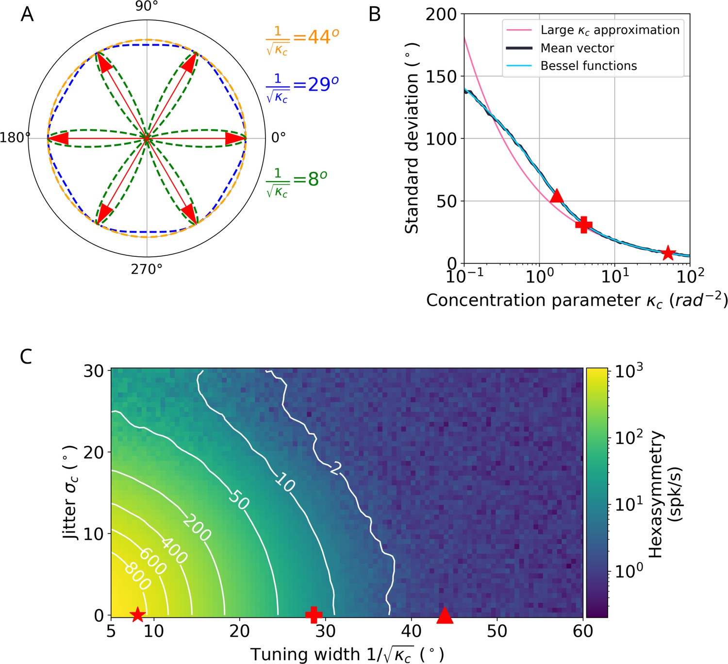
Comparison between the ‘ideal’ tuning width and ‘realistic’ tuning widths found in existing literature for the conjunctive grid by head-direction (HD) cell hypothesis.

(A) Illustration of tuning curves for different tuning widths parameterized using the large- $κ_{c}$ approximation. (B) Comparison between tuning widths using the large- $κ_{c}$ approximation (magenta line) and the tuning widths from Sargolini et al., 2006, which use the mean vector approach (numerical: black line, analytical: blue line). The star corresponds to an angular standard deviation of ${8.1}^{\circ} (κ_{c} = 50)$ , which is the tuning width we use for the ‘ideal’ case in the text. The plus denotes an angular standard deviation of $29^{\circ} (κ_{c} = 4)$ , which is the tuning width we use for the ‘realistic’ case in the text. The triangle marks an angular standard deviation of $55^{\circ} (κ_{c} = 1.7)$ , which is in the range of tuning widths reported by Sargolini et al., 2006 (the large- $κ_{c}$ approximation does not hold in this case, and $55^{\circ}$ angular standard deviation would erroneously correspond to $κ_{c} = 1.1$ ). ‘Mean vector’ in the legend indicates the angular standard deviation calculated using the vector summation of the mean firing rate over angular bins of $6^{\circ}$ . ‘Bessel functions’ denote the angular standard deviation calculated by using a ratio of Bessel functions instead of the resultant vector. See section ‘Tuning widths and the large- $κ$ approximation’ for details on the calculation of the angular standard deviation. (C) Median hexasymmetry (color coded) as a function of HD tuning width (using the large- $κ_{c}$ approximation) and alignment jitter for star-like walk trajectories at an offset of $(0, 0)$ . Higher hexasymmetry values are achieved for stronger HD tuning and tighter alignment of the preferred head directions to the grid axes. The star corresponds to a tuning width of ${8.1}^{\circ} (κ_{c} = 50)$ . The plus represents a tuning width of $29^{\circ} (κ_{c} = 4)$ . The triangle marks a Sargolini-like tuning width of $44^{\circ} (κ_{c} = 1.7)$ , which corresponds to the triangle in panel B. To transform the tuning width from $55^{\circ}$ when using the mean vector method to a tuning width of $44^{\circ}$ when using the large- $κ_{c}$ approximation, the value of $κ_{c}$ for a tuning width of $55^{\circ}$ was found numerically using the ‘mean vector’ curve in panel B. This value of $κ_{c}$ was then used in the expression $1 / \sqrt{κ_{c}}$ to calculate the tuning width in the large- $κ_{c}$ approximation. The units of $1 / \sqrt{κ_{c}}$ have been transformed from radians to degrees by multiplication with a factor $180 / π$ . The hexasymmetry was taken as a median over four trials.

Figure 2—figure supplement 2

Download asset Open asset

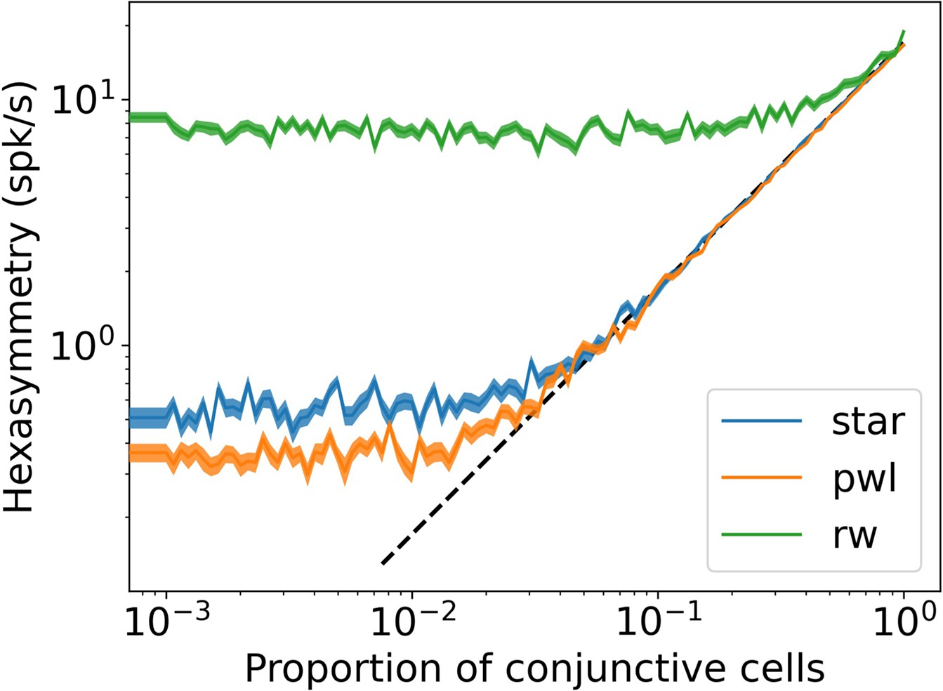
Dependence of the hexasymmetry on the proportion of conjunctive grid by head-direction cells.

The hexasymmetry exhibits a linear dependence on the proportion of conjunctive cells above a noise floor. A black dashed line proportional to $c p_{c}$ is plotted for comparison, where $c = 17$ is an offset parameter chosen to illustrate the linear dependence of the hexasymmetry on the proportion of conjunctive cells for $p_{c} > 0.1$ . In random walks, the noise floor is the contribution of the path hexasymmetry to the neural hexasymmetry. For star-like walks and piecewise linear walks, the noise floor is due to sampling a finite number of grid phase offsets from a uniform distribution on the unit rhombus. The ‘realistic’ parameters were used for each trajectory ( $p_{c} = 0.33$ , $κ_{c} = 4 {rad}^{- 2}$ , $σ_{c} = 3^{\circ}$ ). The shaded area represents the standard error of the hexasymmetry.

Figure 3

Download asset Open asset

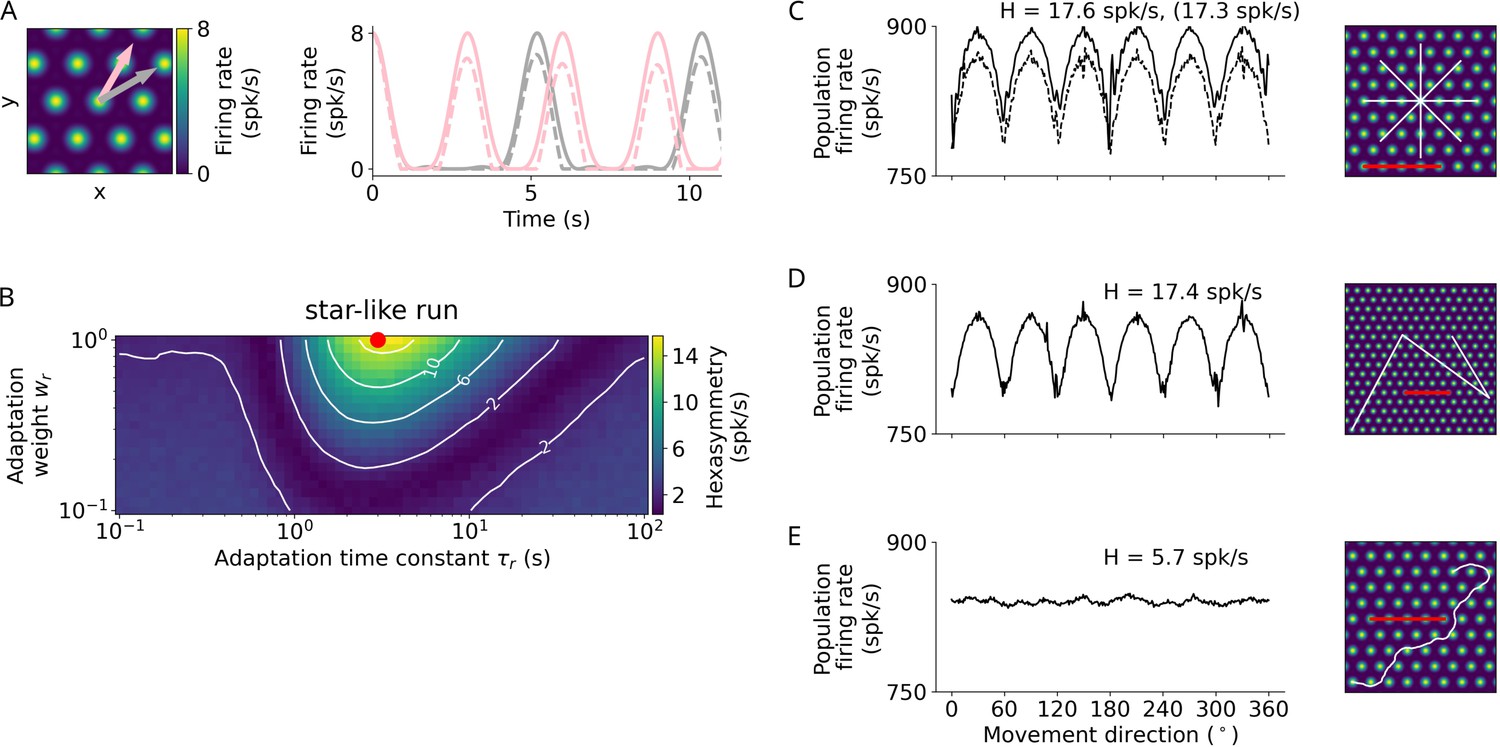
Repetition suppression hypothesis.

(A) Left: Tuning of an example grid cell with aligned (pink arrow) and misaligned (gray arrow) movement directions. Right: Examples of firing-rate adaptation (dashed lines, adaptation weight $w_{r} = 1$ and time constant $τ_{r} = 3$ s) for an aligned run (pink) and a misaligned run (gray). More firing-rate adaptation (i.e. stronger repetition suppression) occurs along the aligned run compared to the misaligned run (attenuation of peaks: 24% and 18% respectively). For both runs, firing rates are reduced compared to the case without adaptation (solid lines). (B) Simulations of hexasymmetry as a function of the weight ( $w_{r}$ ) and time constant ( $τ_{r}$ ) of adaptation for star-like runs. The red dot marks the optimal parameters ( $w_{r} = 1$ and $τ_{r} = 3$ s) used in panels A and C–E. (C) Population firing rate as a function of the subject’s movement direction for a star-like run at an offset of $(0, 0)$ . The solid line represents firing rates for single runs where adaptation does not carry over when sampling different movement directions, i.e., the ‘teleportation’ between path segments resets the repetition suppression effects, and movement directions are sampled consecutively from $0^{\circ}$ to $359^{\circ}$ in steps of $1^{\circ}$ (mean firing rate ${\tilde{A}}_{0} = 866.4$ spk/s, path hexasymmetry $| {\tilde{T}}_{6} | < 10^{- 10}$ ). The dashed line represents firing rates for single runs with adaptation carry-over and randomly sampled movement directions without replacement ( ${\tilde{A}}_{0} = 839.8$ spk/s, path hexasymmetry $| {\tilde{T}}_{6} | < 10^{- 10}$ , the corresponding hexasymmetry is shown in brackets). (D) Population firing rate as a function of movement direction for a piecewise linear walk ( ${\tilde{A}}_{0} = 839.0$ spk/s, $| {\tilde{T}}_{6} | < 10^{- 10}$ ). (E) Population firing rate as a function of movement direction for a random walk ( ${\tilde{A}}_{0} = 839.7$ spk/s, $| {\tilde{T}}_{6} | = 6.7 \cdot 10^{- 3}$ ). spk/s, spikes per second. For all repetition suppression simulations, the grid phase offsets of 1024 grid cells were sampled randomly from a uniform distribution across the unit rhombus, and the hexasymmetries were averaged over 20 realizations. The scale bars (red) in panels C–E represent a distance of 120 cm.

Figure 4 with 1 supplement

Download asset Open asset

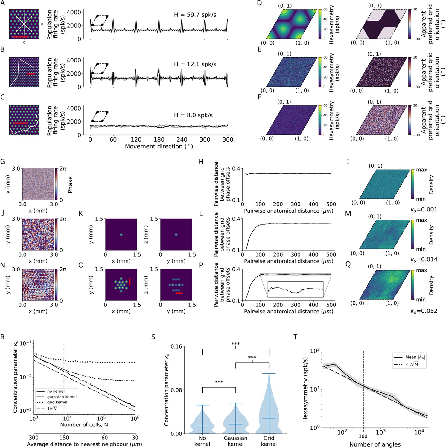
Structure-function mapping hypothesis.

(**A–C**) Left: Short example trajectories (white) overlaid onto the firing-rate pattern of an example grid cell (colored). Shown trajectories are for illustration purposes only, and do not reflect the full length of the simulation. The scale bars (red) represent a distance of 120 cm. Right: Population firing rates of 1024 grid cells as a function of the movement direction. Black and light gray lines represent the results from the numerical simulations of Equation 8 and the analytical derivation in Equation 32, respectively. Grid phase offsets cells are strongly clustered at $(0, 0)$ with $κ_{s} = 10$ (left insets). (A) Left: Subsegment of a star-like walk. Right: Population firing rate as a function of the movement direction for star-like runs originating at phase offset $(0, 0)$ with mean firing rate ${\tilde{A}}_{0} = 1362.4$ spk/s (spikes/second) and path hexasymmetry $| {\tilde{T}}_{6} | < 10^{- 10}$ . (B) Left: Subsegment of a piecewise linear walk. Right: Population firing rate as a function of the movement direction for a piecewise linear trajectory. ${\tilde{A}}_{0} = 1244.3$ spk/s, $| {\tilde{T}}_{6} | < 10^{- 10}$ . (C) Left: Subsegment of a random walk. Right: Population firing rate as a function of movement direction for a random walk. ${\tilde{A}}_{0} = 1305.4$ spk/s, $| {\tilde{T}}_{6} | = 6.7 \cdot 10^{- 3}$ . (D) Left: Hexasymmetry as a function of the subject’s starting location (relative to grid phase offset). Right: Movement direction associated with the highest sum grid-cell activity, i.e., the phase of peaks in (A, right), has a bimodal distribution (0 or 30°). (E) Same as (D) but for piecewise linear walks. (F) Same as (D) but for random walks. (G) Example of a two-dimensional slice of a three-dimensional (3D) random-field simulation with a spatial resolution of 15 μm. The simulated volume of 3 × 3 × 3 mm³ represents the approximate spatial extent of a voxel in functional magnetic resonance imaging (fMRI) experiments (for details, see Methods). (H) The pairwise phase distance in the rhombus is shown as a function of the pairwise anatomical distance for all pairs of simulated cells from (G). Since no spatial correlation structure is induced, the pairwise phase distance between grid cells remains constant when varying the pairwise anatomical distance between them. (I) The resulting phase clustering for 200³ simulated grid cells in a 3 × 3 × 3 mm³ voxel. Brighter colors indicate a higher prevalence of a particular grid phase offset. The distribution of grid phases appears to be homogeneous with a clustering concentration parameter of $κ_{s} = 0.001$ . (**J–M**) Same as (**G–I**) but for a convolution of the 3D random field with the 3D Gaussian correlation kernel of width 30 μm shown in (K). Grid cells located next to each other in anatomical space ( $≲ 30 µm$ ) exhibit similar grid phase offsets (L). No clear clustering is visible, and the fitted clustering concentration parameter was $κ_{s} = 0.014$ (M). (**N–Q**) Same as (**J–M**) but for the grid-like correlation kernel with projections shown in (O), which adds some longer-range spatial autocorrelation to the grid phase offsets of different grid cells. The red bars in (O) measures a distance of 300 μm, which corresponds to the separation between two peaks of the correlation kernel lying on the same plane. The pairwise phase distance (P) exhibits a dip around 300 μm. Note in (Q) that the prevalence of particular grid phase offsets is more biased than in (M), with a fitted clustering concentration parameter of $κ_{s} = 0.052$ . (R) Dependence of the clustering concentration parameter $κ_{s}$ on the number $N$ of grid cells in a voxel. A random distribution of grid cells in anatomical space was obtained by subsampling from the 200³ grid cells simulated in (**G–Q**) over 300 realizations. We found $κ_{s} \approx 0.05$ for 10³ grid cells in a voxel, and that $κ_{s}$ decreases monotonically as $N$ is increased. Convolution of grid phase offsets with a correlation kernel (as in **J–Q**) leads to saturation of $κ_{s}$ for large $N$ . Note that the range of values of $κ_{s}$ here is three orders of magnitude smaller than the strong clustering considered in (**A–C**). The dashed-dotted line depicts the line $1 / \sqrt{N}$ for comparison. The vertical dotted line at $N = 20^{3}$ corresponds to the empirically estimated count of grid cells in a 3 × 3 × 3 mm³ fMRI voxel. The secondary lower horizontal axis shows the average distance between regularly distributed grid cells in anatomical space. (S) The distribution of the clustering concentration parameter $κ_{s}$ when using either no kernel, a Gaussian kernel, or a grid-like kernel for 20³ grid cells subsampled from the 200³ grid cells simulated in (**G–Q**) over 300 realizations. The grid-like kernel results in a larger maximum value of the clustering concentration parameter, and a large number of realizations results in relatively low clustering. ***, p<0.001. (T) The dependence of the hexasymmetry $| {\tilde{A}}_{6} |$ on the number of angles sampled when unwrapping the star for the piecewise linear walk, averaged over 20 trajectories for each data point. Each additional angle sampled adds 300 cm to the total length of the path. A line proportional to $c / \sqrt{M}$ is plotted for comparison, where $c$ is an offset parameter ( $c = 4000$ spk/s) chosen such that the slope of $| {\tilde{A}}_{6} |$ can be compared to the slope of $1 / \sqrt{M}$ , which is proportional to the path hexasymmetry $| {\tilde{T}}_{6} |$ (Equation 67). The close fit between the solid and dashed lines indicates that the neural hexasymmetry $| {\tilde{A}}_{6} |$ is highly correlated with the path hexasymmetry $| {\tilde{T}}_{6} |$ . The vertical dotted line at 360 sampled angles corresponds to the number of angles sampled in the star-like run and the piecewise linear run for all main figures. The value of the clustering concentration parameter used was $κ_{s} = 10$ .

Figure 4—figure supplement 1

Download asset Open asset

Comparison of hexasymmetry resulting from the standard grid cell model (‘standard’) and the structure-function mapping hypothesis (‘Gu’, identical to Figure 5).

Both hypotheses are implemented for three different types of trajectories: star-like walks (‘star’), piecewise linear walks (‘p-l’), and random walks with small step size (‘rand’). For each setting, we show the average neural hexasymmetry $| {\tilde{A}}_{6} |$ for 1024 cells (dark blue bars) and the average contribution of the trajectory $| {\tilde{T}}_{6} | \cdot {\tilde{A}}_{0}$ (light blue bars) where ${\tilde{A}}_{0}$ is the (variable) average population activity and $| {\tilde{T}}_{6} |$ is the hexasymmetry of the trajectory; see Methods for definitions of symbols. The violin plots depict the distributions for firing-rate hexasymmetry (red) and path hexasymmetry (orange). For the ‘standard’ grid cell model, we implemented the structure-function mapping hypothesis, but each realization of the grid phase offsets was sampled from a two-dimensional von Mises distribution with a clustering concentration parameter $κ_{s} = 0$ (equivalent to a uniform distribution on the unit rhombus). In this scenario, random fluctuations give rise to a sample mean clustering concentration parameter of ${\hat{κ}}_{s} = 0.04$ . The sample mean clustering concentration parameter in this case depends on the number of grid cells in a voxel (Figure 4R). Distributing the grid phases regularly throughout the unit rhombus results in ${\hat{κ}}_{s} = 0$ and reduces the mean neural hexasymmetry (star: $5.6 \cdot 10^{- 11}$ spk/s; p-l: $4.8 \cdot 10^{- 11}$ spk/s). Using a constant function (such that each grid cell has the same firing rate for any position of the agent in space) in place of the grid-like firing fields (Equation 2) while sampling the grid phase offsets from a uniform distribution on the unit rhombus similarly reduces the mean neural hexasymmetry (star: $3.6 \cdot 10^{- 11}$ spk/s; p-l: $3.4 \cdot 10^{- 11}$ spk/s). Either regularly distributing the grid phase offsets or using a constant grid function results in a hexasymmetry that is similar in magnitude to the path hexasymmetry. Each hypothesis condition was simulated for 300 realizations. For ‘Gu’ we used $κ_{s} = 0.1$ ; ***, $p < 0.001$ ; n.s., not significant.

Figure 5 with 4 supplements

Download asset Open asset

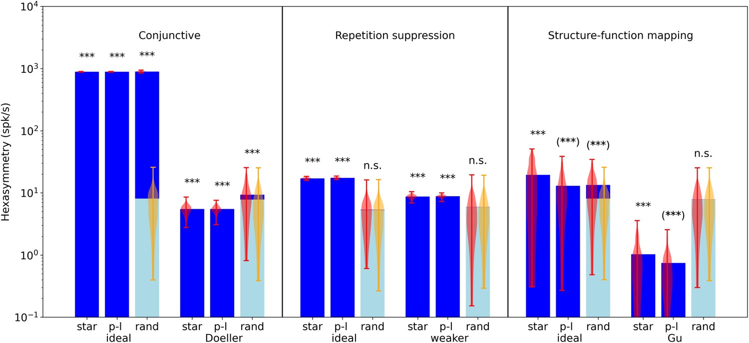
Comparison of hexasymmetry resulting from the three hypotheses.

Each of the three hypotheses is implemented for three different types of navigation trajectories: star-like walks (‘star’), piecewise linear walks (‘p-l’), and random walks with small step size (‘rand’). For each setting, we show the average neural hexasymmetry $| {\tilde{A}}_{6} |$ for 1024 cells (dark blue bars) and the average contribution of the trajectory $| {\tilde{T}}_{6} | \cdot {\tilde{A}}_{0}$ (light blue bars) where ${\tilde{A}}_{0}$ is the (variable) average population activity and $| {\tilde{T}}_{6} |$ is the hexasymmetry of the trajectory; see Methods for definitions of symbols. The violin plots depict the distributions for firing-rate hexasymmetry (red) and path hexasymmetry (orange). For each hypothesis, we calculate the hexasymmetry for ‘ideal’ parameters (conjunctive: $p_{c} = 1$ , $κ_{c} = 50 {rad}^{- 2}$ , tuning width $1 / \sqrt{κ_{c}} = {8.1}^{\circ}$ , $σ_{c} = 0$ ; repetition suppression: $τ_{r} = 3$ s, $w_{r} = 1$ ; clustering: $κ_{s} = 10$ ) as well as more realistic parameters (conjunctive ‘Doeller’: $p_{c} = 0.33$ , $κ_{c} = 4 {rad}^{- 2}$ , tuning width $1 / \sqrt{κ_{c}} = 29^{\circ}$ , $σ_{c} = 3^{\circ}$ motivated by Doeller et al., 2010; Boccara et al., 2010; Sargolini et al., 2006; repetition suppression ‘weaker’: $τ_{r} = 1.5$ s, $w_{r} = 0.5$ ; clustering ‘Gu’: $κ_{s} = 0.1$ motivated by Gu et al., 2018). For clustering, we also simulated grid phase offsets randomly sampled from a uniform distribution with $κ_{s} = 0$ and found that neural hexasymmetries were reduced (compared to ‘Gu’) by $\sim 30 %$ (Figure 4—figure supplement 1). The parameters for the random-walk scenario are $T = 9000$ s and $Δ t = 0.01$ s; see Table 1 for a summary of parameters. Each hypothesis condition was simulated for 300 realizations. ***, p<0.001; n.s., not significant; (***), a seemingly significant result (p<0.001) that we think is spurious (see Results section). For pairwise comparisons of the hexasymmetry values from different trajectory types for each set of parameters, see Figure 5—figure supplement 1. For a quantification of path hexasymmetry as a function of the percentage of subsampled path segments, see Figure 5—figure supplement 2. For a comparison between our method and previously used methods for evaluating hexasymmetry, see Figure 5—figure supplement 4.

Figure 5—figure supplement 1

Download asset Open asset

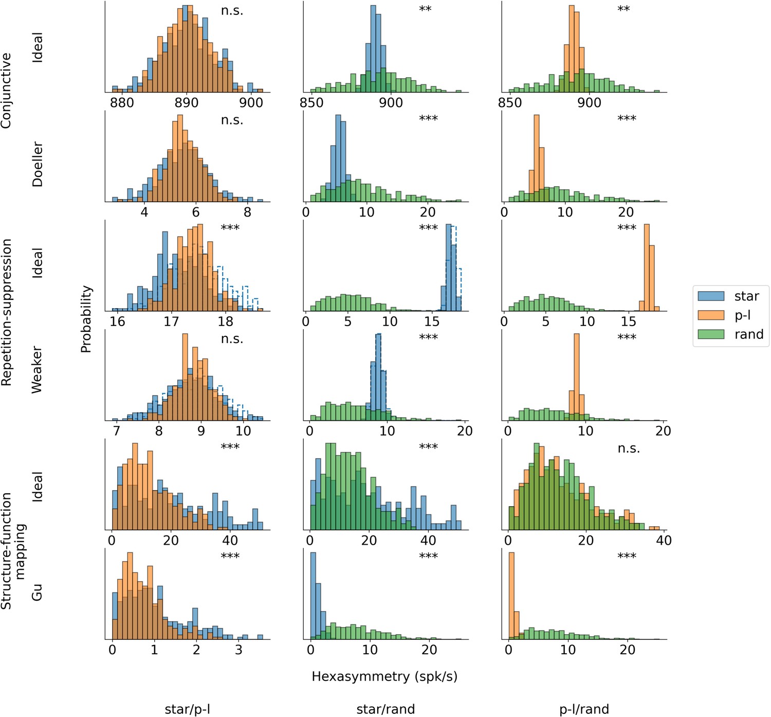
Pairwise comparisons of the hexasymmetry values from different trajectory types for each set of parameters.

The compared trajectory types are star-like walks (‘star’), piecewise-linear walks (‘p-l’), and random walks (‘rand’). For each hypothesis, we calculate the hexasymmetry for ideal parameters (conjunctive: $p_{c} = 1$ , $κ_{c} = 50 {rad}^{- 2}$ ; $σ_{c} = 0$ , repetition suppression: $τ_{r} = 3$ s, $w_{r} = 1$ ; clustering: $κ_{s} = 10$ ) as well as more realistic parameters (conjunctive: $p_{c} = 0.33$ , $κ_{c} = 4 {rad}^{- 2}$ ; $σ_{c} = 3^{\circ}$ repetition suppression: $τ_{r} = 1.5$ s, $w_{r} = 0.5$ ; clustering: $κ_{s} = 0.1$ ). In the case of the repetition suppression hypothesis, the solid blue bars show the star-like walk with a carry-over of the repetition suppression mechanism when teleporting between different path segments, while the transparent bars with the dotted blue borders represent the star-like walk with no carry-over of the repetition suppression effect across different path segments. For the star-like walk, the starting phase of the star is sampled from a uniform distribution across the unit rhombus between realizations, and remains constant within each realization of the star-like walk trajectory. The direction of movement for both the star-like walk and the piecewise linear walk is sampled randomly without replacement from the integer angles ${0, 1, 2, . . ., 359}^{\circ}$ . The parameters for the random-walk scenario are $T = 9000$ s and $Δ t = 0.01$ s. Each hypothesis condition was simulated for 300 realizations. Mann-Whitney U test; ***, p<0.001; **, p<0.01; n.s., not significant. Note that the scales of the horizontal axes are different across subpanels.

Figure 5—figure supplement 2

Download asset Open asset

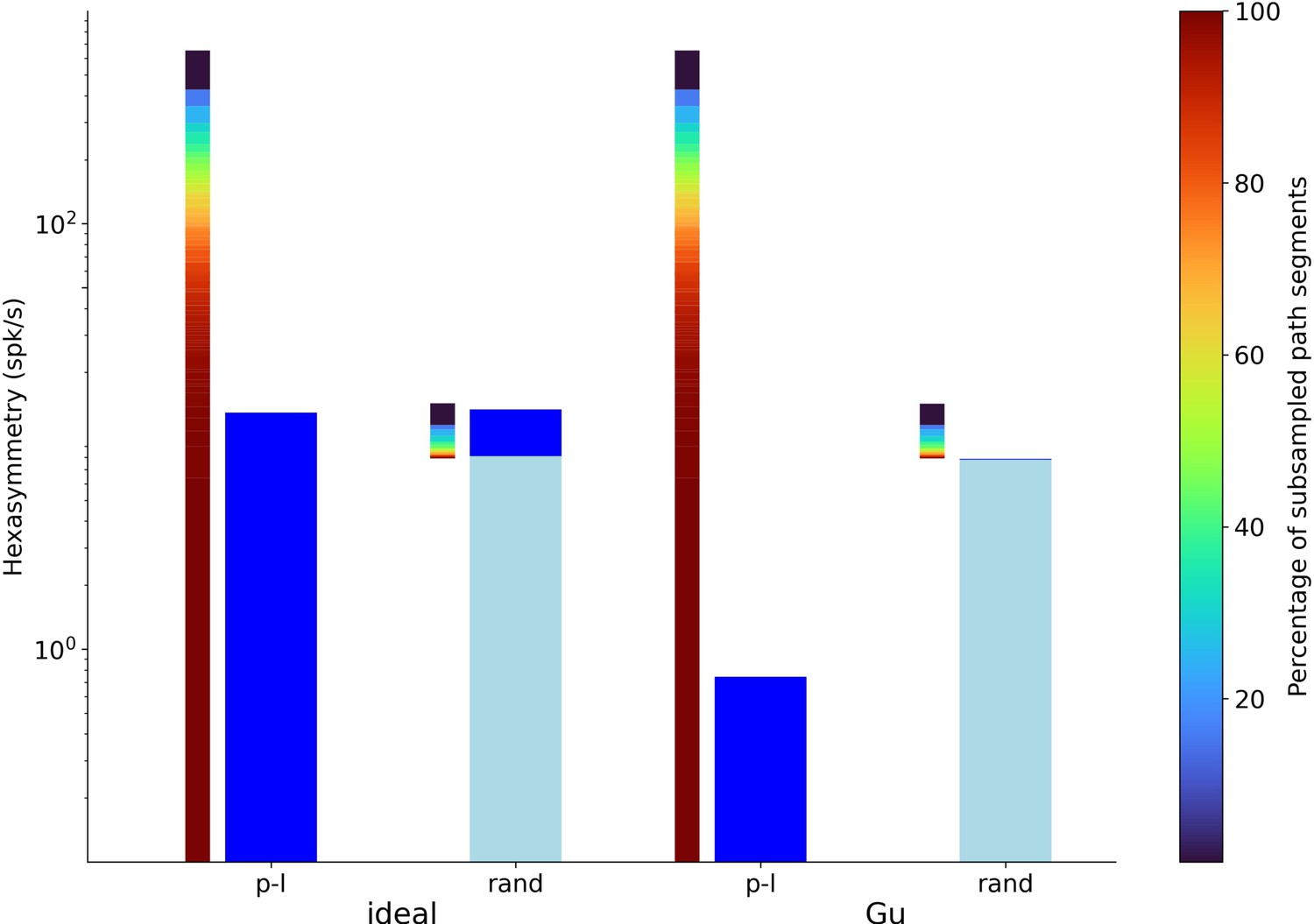
Hexasymmetry resulting from piecewise linear walks (‘p-l’) and random walks (‘rand’) as a function of the percentage of subsampled path segments for the structure-function mapping hypothesis.

Values of ‘ideal’ parameters (left) and more realistic parameter values (‘Gu’; right) are identical to the ones used in Figure 5. The thinner gradient bars show the percentage of subsampled path segments required to produce the corresponding scaled path hexasymmetry $| {\tilde{T}}_{6} | \cdot {\tilde{A}}_{0}$ . The thicker dark blue and light blue bars represent the hexasymmetry $| {\tilde{A}}_{6} |$ and the path hexasymmetry multiplied by the mean firing rate $| {\tilde{T}}_{6} | \cdot {\tilde{A}}_{0}$ , respectively. The percentages of path segments were subsampled from 1% to 100% in steps of 1%. In the case of the random-walk trajectories, e.g., subsampling 100% of the path segments yields $| {\tilde{T}}_{6} | \cdot {\tilde{A}}_{0} = | {\tilde{A}}_{6} | = 7.92$ spk/s. For each percentage value, the path hexasymmetry was averaged over 100 different realizations of the piecewise linear or random-walk trajectory.

Figure 5—figure supplement 3

Download asset Open asset

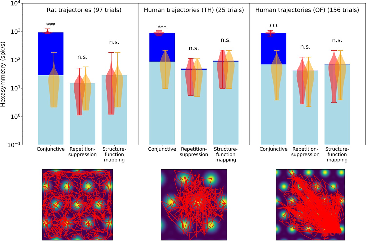
Comparison of the hexasymmetry resulting from the three hypotheses when using trajectories from rats and humans.

For each hypothesis condition, we used 97 rat trajectories (Sargolini et al., 2006) and 181 human trajectories across two datasets (Kunz et al., 2015, Kunz et al., 2021) to estimate neural hexasymmetry and path hexasymmetry. Example trajectories are overlaid on the firing field of a grid cell (bottom panels). The human trajectories were rescaled such that the subject traversed three to four grid firing fields (Hafting et al., 2005) when crossing the environment. For each dataset, the corresponding neural hexasymmetry and path hexasymmetry were evaluated. In the top panel we show for each setting the average neural hexasymmetry $| {\tilde{A}}_{6} |$ for 1024 cells (dark blue bars) and the average contribution of the trajectory $| {\tilde{T}}_{6} | \cdot {\tilde{A}}_{0}$ (light blue bars) where ${\tilde{A}}_{0}$ is the (variable) average population activity; see Methods for definitions of symbols. The violin plots depict the distributions for firing-rate hexasymmetry (red) and path hexasymmetry (orange). While the human trajectories do not result in significant neural hexasymmetry under the repetition suppression hypothesis in this data, we note that there is a variety of different virtual-reality navigation tasks in humans with varying degrees of straightness. For example, in Horner et al., 2016, the navigation paths very clearly resemble piecewise-linear walks. In such studies, repetition suppression effects may play a role in the emergence of grid-like representations. For each hypothesis, we calculated the hexasymmetry for ‘ideal’ parameters (conjunctive: $p_{c} = 1$ , $κ_{c} = 50 {rad}^{- 2}$ ; $σ_{c} = 0$ ; repetition suppression: $τ_{r} = 3$ s, $w_{r} = 1$ ; clustering: $κ_{s} = 10$ ). ***, p<0.001; n.s., not significant.

Figure 5—figure supplement 4

Download asset Open asset

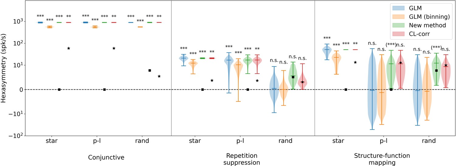
Comparison of hexasymmetry resulting from the three hypotheses when using different methods to calculate the hexasymmetry.

Analogous to Figure 5, each of the three hypotheses (‘conjunctive’, ‘repetition suppression’, ‘structure-function mapping’) is implemented for three different types of trajectories: star-like walks (‘star’), piecewise linear walks (‘p-l’), and random walks with small step size (‘rand’). For each trajectory type within each hypothesis condition, we show four violin plots with the color corresponding to hexasymmetry calculated using different methods: a generalized linear model (‘GLM’, Doeller et al., 2010), a generalized linear model with binning (‘GLM (binning)’, Kunz et al., 2015), our new method (‘New method’), and a circular-linear correlation (‘CL-corr’, Maidenbaum et al., 2018). The mean path hexasymmetry is indicated by a black square. The black star marks the mean hexasymmetry of a surrogate distribution obtained by circularly shifting the firing rates. In all cases, ‘ideal’ parameters were used (conjunctive: $p_{c} = 1$ , $κ_{c} = 50 {rad}^{- 2}$ ; $σ_{c} = 0$ ; repetition suppression: $τ_{r} = 3$ s, $w_{r} = 1$ ; clustering: $κ_{s} = 10$ ). In order to visualize the GLM methods, which can take on negative values, we use the ‘symlog’ scale provided by pyplot, with a linear threshold of ±10 spk/s. Each hypothesis condition for each method was simulated for 300 realizations. Mann-Whitney U test; ***, p<0.001; **, p<0.01; n.s., not significant; for further details, see Methods (Implementation of previously used metrics). For the conjunctive grid by head-direction cell hypothesis, all of the methods find significant neural hexasymmetry for all three types of trajectories, although the circular-linear correlation finds a statistically less significant effect ( $p < 0.01$ for circular-linear correlation, all $p < 0.001$ for other methods). In the case of the repetition suppression hypothesis, all methods find significant neural hexasymmetry for star-like walks and piecewise linear random walks ( $p < 0.01$ for circular-linear correlation, all $p < 0.001$ for the other methods), but find no significant neural hexasymmetry for random walks. With respect to the structure-function mapping hypothesis, all of the methods find significant neural hexasymmetry for star-like walks ( $p < 0.01$ for circular-linear correlation, all $p < 0.001$ for the other methods). For piecewise linear walks and random walks, the new methods detect a spurious significant neural hexasymmetry (labeled ‘(***)’). In section ‘Structure-function mapping hypothesis’, we explain that this spurious effect is due to an inhomogenous sampling of space. All other methods find no significant hexasymmetry under the structure-function mapping hypothesis for piecewise linear walks and random walks. On a side note, when there is significant hexasymmetry, the GLM (binning) method used in Kunz et al., 2015, shows an attenuation in hexasymmetry of roughly 60% due to the averaging effect of binning firing rates into aligned and misaligned movement directions, but this reduction does not change the statistical outcomes. Overall, these observations align with the results obtained through our new method, as depicted in Figure 5.

Author response image 1

Download asset Open asset

Variability of peak firing rates of grid cells when using a random walk trajectory in a finite environment.

(A) Left: The distribution of the peak firing rates for the two conditions (repetition-suppression hypothesis: orange; without repetition-suppression: blue) for 1024 grid cells across 300 simulations and a simulated duration of 9000 seconds, which is kept constant for all panels of (A). Right: The distribution for the coefficient of variation (CV) of the peak firing rates across all cells. The dashed lines represent distribution means. (B) The dependence of the mean CV on the simulated duration for 1024 grid cells across 300 simulations. As the simulated duration increases, the difference in CV between the two cases decreases. The shaded area represents the standard error. (C) Four examples of the rate map for different values of the simulated duration. In the rightmost panel, the trajectory is not shown so that the rate map can be seen clearly. We employed the 'ideal’ parameter set for repetition suppression: τr = 3 s, wr = 1; in all simulations, cells did not show any head direction-tuning, and there was no clustering of grid-phase offsets. The size of the environment was limited to a square with side lengths of 100 cm. Mann-Whitney U test; ***, P < 0.001; **, P < 0.01; *, P < 0.05; n.s., not significant.

Tables

Table 1

Parameters: descriptions and values.

For a more detailed motivation of the values used, see section ‘Parameter estimation’.

Parameter	Description	Values (unless varied) or range
	Trajectories
$Δ t$	Simulation time step	0.01 s
$T$	Simulated duration	9000 s
$v$	Movement speed	10 cm/s
$σ_{θ}$	Movement tortuosity	0.5 rad/s^1/2
$r_{m a x}$	Length of a linear path in the star-like run	300 cm
$N_{θ}$	Number of angles to sample in the star-like run	360
	Grid cells
$N$	Number of grid cells in a voxel	1024
$s$	Grid scale	30 cm
$γ$	Grid orientation	0°
$A_{m a x}$	Maximum firing rate for one grid cell	8 spk/s
$(x_{off}, y_{off})$	Grid phase (two-dimensional)	([0,1], [0,1])
	Conjunctive grid by head-direction cell hypothesis
$μ_{c}$	Preferred head direction	$[0, 2 π)$ (multiples of 60° for $σ_{c} = 0$ )
$κ_{c}$	Concentration parameter for direction tuning for the ideal and ‘realistic’ cases	{50, 4} rad^-2
$σ_{c}$	Alignment jitter of direction tuning to grid axis for the ideal and ‘realistic’* cases	{0, 3}°
$p_{c}$	Fraction of conjunctive cells in a population for the ideal and ‘realistic’* cases	{1, 1/3}
	Repetition suppression hypothesis
$τ_{r}$	Adaptation time constant for the ideal and ‘weaker’ cases	{3, 1.5} s
$w_{r}$	Adaptation weight for the ideal and ‘weaker’ cases	{1, 0.5}
	Structure-function mapping hypothesis
$μ_{s}$	Central phase of cluster	(0, 0)
$κ_{s}$	Concentration parameter for clustering for the ideal and ‘realistic’^† cases	{10, 0.1}

*

Boccara et al., 2010; Sargolini et al., 2006.
†

Gu et al., 2018.

Additional files

MDAR checklist: https://cdn.elifesciences.org/articles/85742/elife-85742-mdarchecklist1-v1.docx
Download elife-85742-mdarchecklist1-v1.docx

Download links

A two-part list of links to download the article, or parts of the article, in various formats.

Downloads (link to download the article as PDF)

Open citations (links to open the citations from this article in various online reference manager services)

Mendeley

Cite this article (links to download the citations from this article in formats compatible with various reference manager tools)

Ikhwan Bin Khalid
Eric T Reifenstein
Naomi Auer
Lukas Kunz
Richard Kempter

(2024)

Quantitative modeling of the emergence of macroscopic grid-like representations

eLife 13:e85742.

https://doi.org/10.7554/eLife.85742

Share this article

Cite this article

Qualitative hypotheses on the emergence of macroscopic grid-like representations in the human entorhinal cortex.

Effect of tortuosity on the hexasymmetry for the repetition suppression hypothesis with random walks (Δt=0.01s s, T=9000s, τr=3s, wr=1).

Effect of size and shape of finite environments on hexasymmetry.

Effect of rotation of finite environments on hexasymmetry.

Hexasymmetry of random-walk trajectories.

Conjunctive grid by head-direction (HD) cell hypothesis.

Comparison between the ‘ideal’ tuning width and ‘realistic’ tuning widths found in existing literature for the conjunctive grid by head-direction (HD) cell hypothesis.

Dependence of the hexasymmetry on the proportion of conjunctive grid by head-direction cells.

Repetition suppression hypothesis.

Structure-function mapping hypothesis.

Comparison of hexasymmetry resulting from the standard grid cell model (‘standard’) and the structure-function mapping hypothesis (‘Gu’, identical to Figure 5).

Comparison of hexasymmetry resulting from the three hypotheses.

Pairwise comparisons of the hexasymmetry values from different trajectory types for each set of parameters.

Hexasymmetry resulting from piecewise linear walks (‘p-l’) and random walks (‘rand’) as a function of the percentage of subsampled path segments for the structure-function mapping hypothesis.

Comparison of the hexasymmetry resulting from the three hypotheses when using trajectories from rats and humans.

Comparison of hexasymmetry resulting from the three hypotheses when using different methods to calculate the hexasymmetry.

Variability of peak firing rates of grid cells when using a random walk trajectory in a finite environment.

Parameters: descriptions and values.

MDAR checklist

Downloads (link to download the article as PDF)

Open citations (links to open the citations from this article in various online reference manager services)

Cite this article (links to download the citations from this article in formats compatible with various reference manager tools)

Effect of tortuosity on the hexasymmetry for the repetition suppression hypothesis with random walks ( $Δ t = 0.01 s$ s, $T = 9000 s$ , $τ_{r} = 3 s$ , $w_{r} = 1$ ).