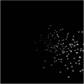
Towards biologically plausible phosphene simulation for the differentiable optimization of visual cortical prostheses
Figures

Left: schematic illustration of our simulator pipeline.
Our simulator is initialized with electrode locations on a visuotopic map of the visual cortex. Each frame, the simulator takes a set of stimulation parameters that for each electrode specify the amplitude, pulse width, and frequency of electrical stimulation. Based on the electrode locations on the cortical map and the stimulation parameters, the phosphene characteristics are estimated and for each phosphene the effects are rendered on a map of the visual field. Finally, the phosphene renderings are summed to obtain the resulting simulated prosthetic percept. Right: Example renderings after initializing the simulator with four 10 × 10 electrode arrays (indicated with roman numerals) placed in the right hemisphere (electrode spacing: 0.4 mm, in correspondence with the commonly used ‘Utah array’ Maynard et al., 1997). The output is visualized for 166 ms pulse trains with stimulation amplitudes of 40, 80, and 120 µA, a pulse width of 170 ms, and a frequency of 300Hz. In these example frames, we can observe the effects of cortical magnification, thresholds for activation, current-dependent spread (size) and proportion (brightness) of cortical tissue activation.
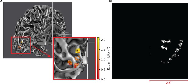
Demonstration of the use of the simulator in conjunction with external software for receptive field prediction (Goebel et al., 2006).
(A) On the left, a 3D brain model with receptive field mapping (color indicates eccentricity in the visual field) is used to simulate the placement of four 8-by-8 Utah-like electrode arrays on the accessible parts of visual cortex (V1) in the left hemisphere. The inset shows a close-up of the electrodes and the expected locations of the visual receptive fields (color indicates eccentricity). (B) On the right, we see the resulting simulation of stimulating these electrodes with a current amplitude of 70 µA, after 167 ms of continuous stimulation. To simulate imperfect knowledge of the electrode or phosphene locations, a small normally distributed noise () was added to the determined receptive fields. Note that as the simulator is initialized with the phosphene locations in the visual field, any assumptions about feasible electrode locations, uncertainties, and other sources of noise can be incorporated flexibly.

Example simulation of irregular phosphene shapes.
In our software, it is relatively straightforward to change the shape of individual phosphenes. The simulator includes the functionality of initializing with elongated phosphenes and the phosphene maps can also be manually adjusted to simulate arbitrary shapes. (A) Schematic illustration of the modeled visual field location. (B) The simulation output after initialization with 50 elongated phosphenes with random orientations. (C) Simulation output with manually customized phosphene shapes.

Example simulations of irregular phosphene percepts that can arise upon multi-electrode stimulation of three electrodes.
By default, the simulator assumes independence between electrodes and their corresponding percepts. However, the code can be easily customized to simulate interactions between electrodes. In each of these examples, the base input is a stimulation vector describing the activation of three electrodes with a current of 100 µA. The pulse width was set to 170 µs, and the frequency was set to 300 Hz. Before being sent to the simulator, the stimulation vector is processed by different custom interaction models. (A) No interactions: the input is multiplied with the identity matrix before feeding to the simulator, resulting in phosphenes I, II, and III. (B) Coactivation: phosphenes I and II are activated by a weighted sum of the first two electrodes, simulating a ‘leak’ between the electrodes, resulting in brighter phosphenes. (C) Merging: a non-linear interaction model is used consisting of a two-layer fully connected network with ReLU activation. When simultaneously activated, phosphenes I and II are replaced by a phosphene that falls in between the original locations. (D) Arbitrary percept: similar to panel (C), the percepts of phosphenes I and II are replaced by a new percept when simultaneously activated. The new percept is an oblique line.
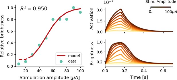
Estimate of the relative phosphene brightness for different stimulation amplitudes.
The simulator was provided with a stimulation train of 166 ms with a pulse width of 170 µs at a frequency of 300 Hz (see Equations 7, 8, 9 and 10). Left: the fitted brightness levels reproduced by our model (red) and psychometric data reported by Fernández et al., 2021 (light blue). Note that for stimulation amplitudes of 20 µA and lower, the simulator generated no phosphenes as the threshold for activation was not reached. Right: the modeled tissue activation and brightness response over time.
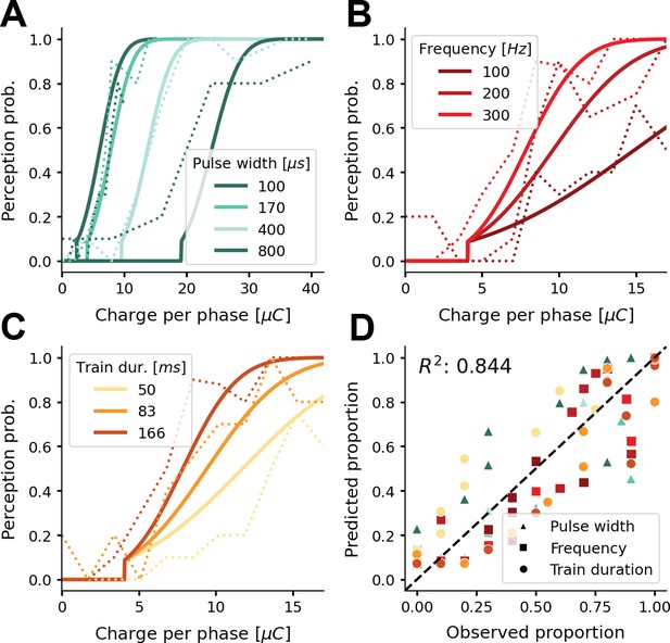
Probability of phosphene perception for different stimulation parameters.
(A–C) Psychometric curves (solid lines) overlaid on experimental data (dashed lines) (Fernández et al., 2021; Figure 2a and b). The model’s probability of phosphene perception is visualized as a function of charge per phase for (A) different pulse widths, (B) different frequencies, and (C) different train durations. Note that rather than the total charge per trial, we report the charge per phase to facilitate easy comparison with aforementioned experimental data. In panel (D) the probabilities of phosphene perception reproduced with our model are compared to the detection probabilities reported in (Fernández et al., 2021; Figure 2a and b). Predicted probabilities in panel (D) are the results of a threefold cross-validation on held-out test data. Colors conform to the conditions in panels A, B, and C.
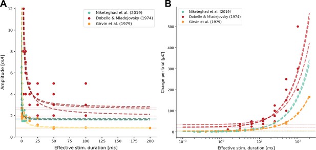
Sixfold cross-validation results of fitting the simulator to data from several clinical studies that used cortical surface electrodes (Dobelle and Mladejovsky, 1974; Girvin et al., 1979; Niketeghad et al., 2020).
The predicted current threshold (A) and total charge threshold (B) are displayed as a function of the effective stimulation duration. The model fit (dashed lines) is overlaid on several sources of experimental data (solid points) from Niketeghad et al., 2020 (), Dobelle and Mladejovsky (), and Girvin et al., 1979 (). In the respective publications, experimental data were read out from graphs (Niketeghad et al., 2020; Girvin et al., 1979) and tables (Dobelle and Mladejovsky, 1974).
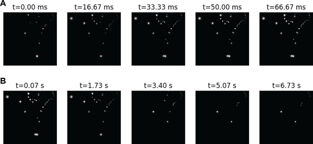
Demonstration of the effect of the model’s temporal dynamics over time.
Stimulation currents between 5 and 180 µA were simulated for 7s, using a pulse width of 170 µs at a frequency of 300 Hz. The figures show the lower left quadrant of the visual field, where 130 phosphenes are located. (A) The first five frames of the simulation, show the delayed onset of phosphenes and increase in brightness. (B) Frames at subsequent regular intervals, showing gradual phosphene fading.
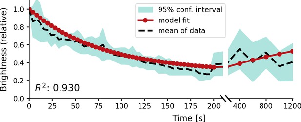
Relative brightness of a phosphene in response to repeated stimulation, overlaid on experimental results by Schmidt et al., 1996.
The stimulation sequence consisted of 50 pulse trains at a 4 s stimulation interval, followed by five pulse trains at an interval of 200 s to test recovery. The simulator was provided with a stimulation train of 125 ms with a pulse width of 100 µs at a frequency of 200 Hz using a stimulation amplitude of 90 µA. Please notice the split x-axis with variable scaling.
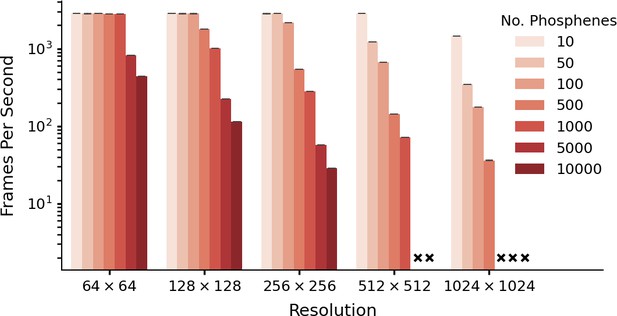
Performance as a function of resolution and number of phosphenes.
The data is based on five runs of 1540 frames per condition, with batch size equal to one frame. Simulation was run with an NVIDIA A30 GPU (memory size: 24 GB). Crosses indicate missing conditions. Note that these data are presented only for evaluating the software-performance. For some combinations of phosphene count and image resolution (e.g. 10.000 phosphenes in a 64 × 64 image) there are fewer pixels than phosphenes. The error bars indicate the 95-percent confidence interval.
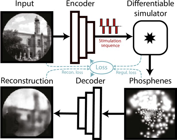
Schematic illustration of the end-to-end machine-learning pipeline adapted from de Ruyter van Steveninck et al., 2022a.
A convolutional neural network encoder is trained to convert input images or video frames into a suitable electrical stimulation protocol. In the training procedure, the simulator generates a simulation of the expected prosthetic percept, which is evaluated by a second convolutional neural network that decodes a reconstruction of the input image. The quality of the encoding is iteratively optimized by updating the network parameters using back-propagation. Different loss terms can be used to constrain the phosphene encoding, such as the reconstruction error between the reconstruction and the input, a regularization loss between the phosphenes and the input, or a supervised loss term between the reconstructions and some ground-truth labeled data (not depicted here). Note that the internal parameters of the simulator (e.g. the estimated tissue activation) can also be used as loss terms.
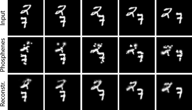
Results of training the end-to-end pipeline on video sequences from the moving MNIST dataset (Srivastava et al., 2015).
Columns indicate different frames. Top row: the input frames; middle row: the simulated phosphene representations; bottom row: the decoded reconstructions of the input.
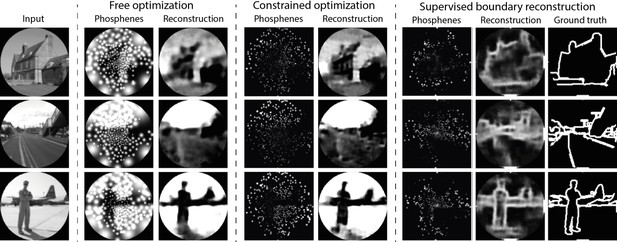
Results of training our simulator in an end-to-end pipeline on naturalistic images from the ADE20K dataset (Zhou et al., 2019).
In the constrained optimization condition and the supervised boundary reconstruction condition, the encoder was configured to output 10 discrete stimulation amplitudes within the safe range of stimulation (0 to 128 µA). The selected images represent the first three categories in the validation dataset (‘Abbey’, ‘Access Road,’ ‘Airbase’). Note that the brightness is enhanced in the phosphene images of the constrained optimization and the supervised boundary condition by 40%. (See Figure 8—figure supplement 1 and Figure 8—figure supplement 2 for enlarged and inverted simulated prosthetic vision (SPV) images).
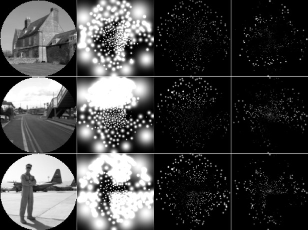
Enlarged version of the simulated prosthetic vision (SPV) representations in Figure 8.
From left to right, the columns indicate: the input images; the SPV representations in the unconstrained optimization condition; the SPV representations in the constrained optimization condition; the SPV representations in the supervised boundary reconstruction condition.
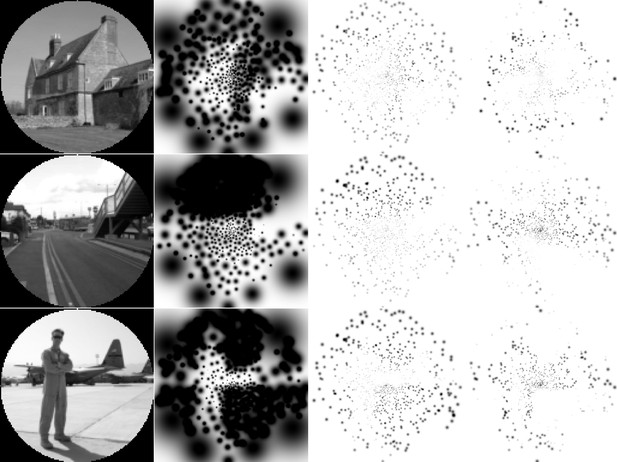
Inverted grayscale version of the simulated prosthetic vision (SPV) representations in Figure 8.
From left to right, the columns indicate: the input images; the SPV representations in the unconstrained optimization condition; the SPV representations in the constrained optimization condition; the SPV representations in the supervised boundary reconstruction condition.
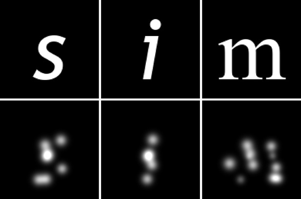
Example results after training an end-to-end model with a small electrode count.
The simulator was initialized with a random subset of 60 electrodes from a 10 × 10 array with electrode spacing of 0.4 mm, matching the location and spacing of array no. IV in Figure 1. The model was trained on an image dataset of white characters on a black background. The top row displays three example inputs, and the bottom row shows the simulated prosthetic vision SPV encoding found by the encoder model after training.
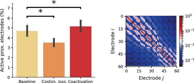
Results after training an end-to-end model on a small electrode count (60 electrodes) with different interaction conditions.
In the baseline condition, the model was trained without electrode interactions. In the costimulation loss condition, no electrode interactions were simulated, but an additional loss component was introduced to discourage simultaneous activation of neighboring electrode pairs. In the coactivation condition, no additional loss function was used, but an interaction model was implemented in the simulator. For each active electrode, a coactivation leak current was added from neighboring electrodes. Left panel: the percentage of active electrode pairs with a relative distance smaller than 1 mm. Costimulation loss resulted in significantly smaller number of active neighboring electrode pairs. Adding a coactivation current resulted in a significant increase of simultaneously active neighboring electrodes. (p < 0.001 for both comparisons with the baseline condition). The error bars indicate the 95-percent confidence interval. Right panel: the coactivation matrix characterizing the magnitude of the leak current between electrodes in the coactivation condition.


