Enhancing precision in human neuroscience
Figures
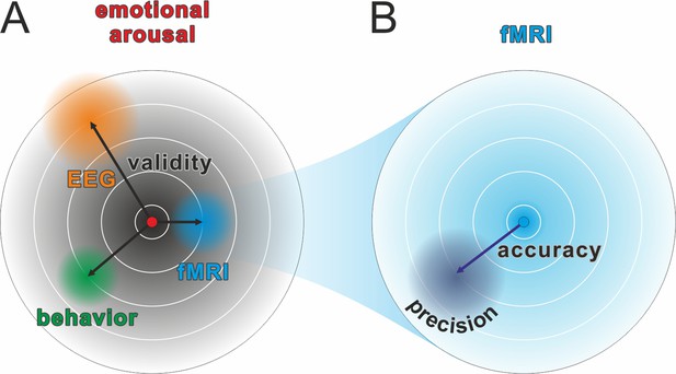
Comparison of validity, precision, and accuracy.
(A) A latent construct such as emotional arousal (red dot in the center of the circle) can be operationalized using a variety of methods (e.g., EEG ERN amplitudes, fMRI amygdala activation, or self-reports such as the Self-Assessment Manikin). These methods may differ in their construct validity (black arrows), that is, the measurement may be biased away from the true value of the construct. Of note, in this model, the true values are those of an unknown latent construct and thus validity will always be at least partially a philosophical question. Some may, for example, argue that measuring neural activity directly with sufficient precision is equivalent to measuring the latent construct. However, we prescribe to an emergent materialism and focus on measurement precision. The important and complex question of validity is thus beyond the scope of this review and should be discussed elsewhere. (B) Accuracy and precision are related to validity with the important difference that they are fully addressed within the framework of the manifest variable used to operationalize the latent construct (e.g., fMRI amygdala activation). The true value is shown as a blue dot in the center of the circle and, in this example, would be the true activity of the amygdala. The lack of accuracy (dark blue arrow) is determined by the tendency of the measured values to be biased away from this true value, that is, when signal losses to deeper structures alter the blood oxygen-level dependent (BOLD) signal measuring amygdala activity. Oftentimes, accuracy is unknown and can only be statistically estimated (see Eye-Tracking section for an exception). The precision is determined by the amount of error variance (diffuse dark blue area), i.e. precision is high if BOLD signals measured at the amygdala are similar to each other under the assumption that everything else remains equal. The main aim of this review is to discuss how precision can be optimized in human neuroscience.
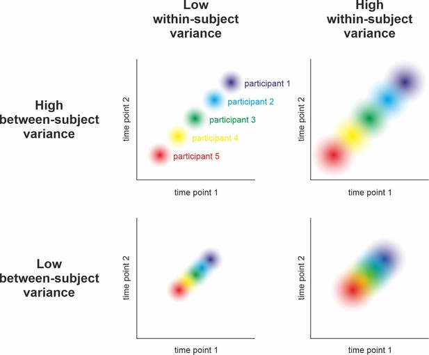
Relation between reliability and precision.
Hypothetical measurement of a variable at two time points in five participants under different assumptions of between-subjects and within-subject variance. Reliability can be understood as the relative stability of individual z-scores across repeated measurements of the same sample: Do participants who score high during the first assessment also score high in the second (compared to the rest of the sample)? Statistically, its calculation relies on relating the within-subject variance (illustrated by dot size) to the between-subjects variance (i.e., the spread of dots). As can be seen above and in , high reliability is achieved when the within-subject variance is small and the between-subjects variance is large (i.e., no overlap of dots in the top left panel). Low reliability can occur due to high within-subject variance and low between-subjects variance (i.e., highly overlapping dots in the bottom right) and intermediate reliability might result from similar between- and within-subject variance (top right and bottom left). Consequently, reliability can only be interpreted with respect to subject-level precision when taking the observed population variance (i.e., the group-level precision) into account (see ). For example, an event-related potential in the EEG may be sufficiently reliable after having collected 50 trials in a sample drawn from a population of young healthy adults. The same measure, however, may be unreliable in elderly populations or patients due to increased within-subject variance (i.e., decreased subject-level precision).
-
Figure 2—source code 1
Reliability, between & within variance.
This R code simulates four samples of 50 subjects with 50 trials each using different degrees of variability within and between subjects. The results indicate that (odd-even) reliability is best at a combination of low within-subject variance but high between-subjects variability (leading to lower group-level precision). Reliability declines when within- and between-subjects variance are both high or low and is worst when the former is high but the latter is low. The results support the claims illustrated in Figure 2.
- https://cdn.elifesciences.org/articles/85980/elife-85980-fig2-code1-v1.zip
-
Figure 2—source code 2
Reliability & (between) SD.
This R code simulates two samples of 64 subjects with 100 trials each using vastly different degrees of between-subjects variance (but constant within-subject variability, leading to constant subject-level precision). The results show that, everything else being equal, homogenous samples (i.e., with low between-subjects variance) optimize group-level precision at the expense of reliability (Hedge et al., 2018), while heterogenous samples optimize reliability at the expense of group-level precision.
- https://cdn.elifesciences.org/articles/85980/elife-85980-fig2-code2-v1.zip
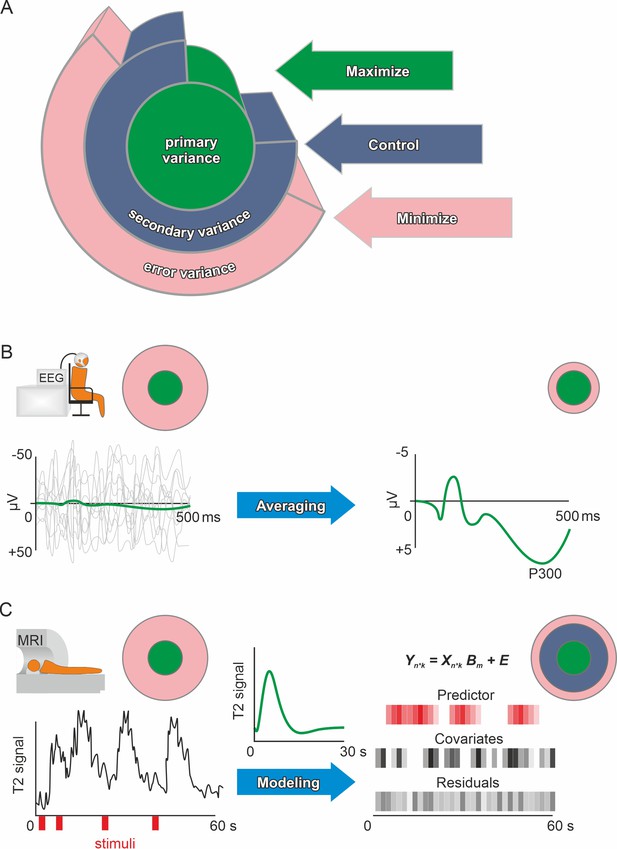
Primary, secondary, and error variance.
(A) There are three main sources of variance in a measurement, each providing a different angle on optimizing precision. Primary (or systematic) variance results from changes in the true value of the manifest (dependent) variable upon manipulation of the independent variable and therefore represents what we desire to measure (e.g., neuronal activity due to emotional stimuli). Secondary variance is attributable to other variables that are not the focus of the research but are under the experimenter’s control, for example, the influence of the menstrual cycle on neural activity can either be controlled by measuring all participants at the same time of the cycle or by adding time of cycle as a covariate to the analysis. Trivially, if the research topic was the effect of the menstrual cycle on neural activity, then this variance would be primary variance, highlighting that these definitions depend solely on the research question. Error variance is any change in the measurement that cannot be reasonably accounted for by other variables. It is thus assumed to be a random error (see systematic error for exceptions). Explained variance (see definition of effect size in the Glossary in Appendix) is the size of the effect of manipulating the independent variable compared to the total variance after accounting for the measured secondary variance (via covariates). Precision is enhanced if the error variance is minimized and/or the secondary variance is controlled. Methods in human neuroscience differ substantially in the way they deal with error variance. (Kerlinger, 1964, for the first description of the Max-Con-Min principle). (B) In EEG research, a popular method is averaging. On the left, the evoked neuronal response (primary variance – green line) of an auditory stimulus is much smaller than the ongoing neuronal activity (error variance – gray lines). Error variance is assumed to be random and, thus, should cancel out during averaging. The more trials (many gray lines on the left) are averaged, the less error variance remains if we assume that the underlying true evoked neuronal response remains constant (green subject-level evoked potential on the right). Filtering and independent component analysis are further popular methods to reduce error variance in EEG research. After applying these procedures on the subject-level, the data can be used for group-level analyses. (C) In fMRI research, a linear model is commonly used to prepare the subject-level data before group analyses. The time series data are modeled using beta weights, a design matrix, and the residuals (see GLM and mass univariate approaches in the Glossary in Appendix). Essentially, a hypothetical hemodynamic response (green line in the middle) is convolved with the stimuli (red) to form predicted values. Covariates such as movements or physiological parameters are added. Therefore, the error variance (residuals) that remains is the part of the time series that cannot be explained by primary variance (predictor) or secondary variance (covariates). Of course, averaging and modeling approaches can both be used for the same method depending on the researcher’s preferences. Additionally, pre-processing procedures such as artifact rejection are used ubiquitously to reduce error variance.
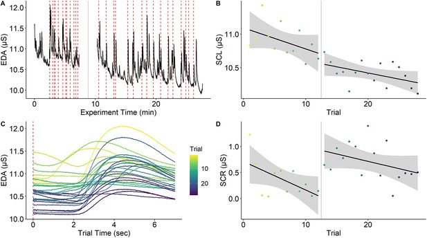
Habituation of electrodermal activity.
Habituation of electrodermal activity (EDA) is illustrated using a single subject from Reutter and Gamer, 2023. (A) EDA across the whole experiment with the red dashed lines marking onsets of painful stimuli and the gray solid line denoting a short break between experimental phases. (B) Skin conductance level (SCL) across trials (separately for experimental phases) showing habituation (i.e., decreasing SCLs) across the experiment. (C) Trial-level EDA after each application of a painful stimulus showing that SCL and skin conductance response (SCR) amplitude is reduced as the experiment progresses. (D) SCRs (operationalized as baseline-to-peak differences) decrease over time within the same experimental phase. Interestingly, SCR amplitudes ‘recover’ at the beginning of the second experimental phase even though this is not the case for SCL. Notably, this strong habituation of SCL and SCR means that increasing trials for higher precision may not always be possible. However, the extent to which components of primary and error variance are reduced by habituation remains an open question. This figure can be reproduced using the data and R script in ‘Figure 4—source data 1’.
-
Figure 4—source data 1
This zip archive contains EDA data (‘eda.txt’) and rating data (‘ratings.csv’), which are loaded and processed in the R script ‘Habituation R’ to reproduce Figure 4.
The R script also contains examples on how to calculate precision for SCL and SCR. The data have been reused with permission from Reutter and Gamer, 2023.
- https://cdn.elifesciences.org/articles/85980/elife-85980-fig4-data1-v1.zip
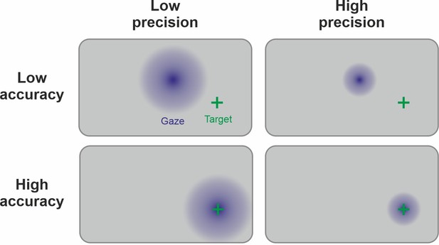
Link between precision and accuracy of gaze signal.
Due to the physiology of the eye, the ground truth of the manifest variable (fixation) is known during the calibration procedure. Therefore, accuracy and precision can be disentangled by this step. Accuracy is high if the calibration procedure leads to estimated gaze points (in blue) being centered around the target (green cross). Precision is high if the gaze points are less spread out. Ideally, both high precision and high accuracy are achieved. Note that the precision and accuracy of the measurement can change significantly after the calibration procedure, for example, because of participant movement.
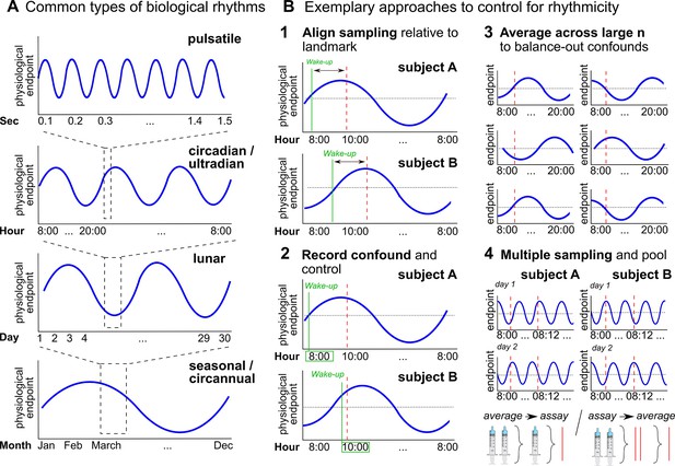
Biological rhythms and how to control for them.
(A) Examples of biological rhythms. Pulsatile rhythms refer to cyclic changes starting within (milli)seconds, ultradian rhythms occur in less than 20 hr, whereas circadian rhythms encompass changes within a day approximately. These rhythms are intertwined (Young et al., 2004) and included in even longer rhythms, such as occurring within a week (circaseptan), within 20–30 days (lunar; prominent example is the menstrual cycle), within a season (seasonal), or within one year (circannual). (B) Exemplary approaches to account for biological rhythms. Time of day at sampling, in itself and relative to awakening, is especially important when implementing physiological measures with a circadian rhythm (Nader et al., 2010; Orban et al., 2020) and needs to be controlled (B1-2). For trait measures, reliability can be increased by collecting multiple samples across participants of the same group, and/or better within participants (B3-4; Schmalenberger et al., 2021).
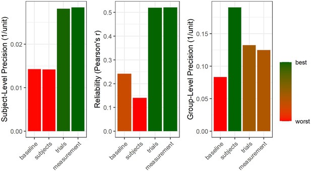
Hierarchical structure of precision.
Four samples were simulated at different degrees of precision on group-, subject-, and trial-level. We start with a baseline case for which all levels of precision are comparably low (64 subjects, 50 trials per subject, 500 arbitrary units of random noise on trial-level). Afterwards, the number of subjects is quadrupled to double group-level precision (right panel) but no effect on subject-level precision or reliability is observed (a descriptive drop in reliability is due to sampling error). Subsequently, the number of trials is quadrupled to double subject-level precision. This also increases reliability and, vitally, carries on to improve group-level precision (Baker et al., 2021), albeit to a smaller extent than increasing sample size by the same factor. Finally, the trial-level deviation from the true subject-level means is halved to double trial-level precision. This improves both subject-level and group-level precision without increasing the number of data points (i.e., subjects or trials).
-
Figure 7—source code 1
This R code can be used to reproduce Figure 7.
- https://cdn.elifesciences.org/articles/85980/elife-85980-fig7-code1-v1.zip
Additional files
-
Supplementary file 1
Resources.
- https://cdn.elifesciences.org/articles/85980/elife-85980-supp1-v1.docx


